Study on double-shaft mixing paddle undergoing planetary motion in the laminar flow mixing system

Abstract

This article has studied the impact of double-shaft mixing paddle undergoing planetary motion on laminar flow mixing system using flow field visualization experiment and computational fluid dynamics simulation. Digital image processing was conducted to analyze the mixing efficiency of mixing paddle in co-rotating and counter-rotating modes. It was found that the double-shaft mixing paddle undergoing planetary motion would not produce the isolated mixing regions in the laminar flow mixing system, and its mixing efficiency in counter-rotating modes was higher than that in co-rotating modes, especially at low rotating speed. According to the tracer trajectory experiment, it was found that the path line of the tracer in the flow field in co-rotating modes was distributed in the opposite direction to the path line in counter-rotating modes. Planetary motion of mixing paddle had stretching, shearing, and folding effects on the trajectory of the tracer. By means of computational fluid dynamics simulation, it was found that axial flows and tangential flows produced in co-rotating and counter-rotating modes have similar flow velocity but opposite flow directions. It is deduced from the distribution rule of axial flow, radial flow, and tangential flow in the flow field that axial flow is the main reason for causing different mixing efficiencies between co-rotating and counter-rotating modes.

Introduction

Mixing process is widely used in chemical, biological, pharmaceutical, petroleum, and food industries. The mixing flow field can be distinguished into laminar flow, transition flow, and turbulent flow field according to different Re. In the laminar flow mixing system, the mixed object has poor time-dependent behavior due to viscous force. In particular, during laminar flow mixing at low Re, distinct isolated mixing regions (IMRs) often form in the vicinity of the mixing paddle. Therefore, it takes a lot of mixing time and energy to achieve uniform mixing. ¹ Many researchers have conducted a lot of studies on the laminar flow mixing process, with an aim to eliminate the IMRs and improve mixing efficiency.

Flow field visualization experiment is an effective way to study the laminar flow mixing process. Flow field visualization experiments include acid–base neutralization and color change experiment, fluorescent tracer experiment, particle image velocimetry (PIV) experiment, and planar laser-induced fluorescence (PLIF) experiment. Lamberto et al. ² effectively eliminated IMRs generated by acid–base neutralization experiment via changing rotating speed and improved the efficiency of laminar flow mixing at low Re. Alvarez et al. ³ conducted acid–base neutralization experiment, two-dimensional (2D) PLIF experiment, and three-dimensional (3D) ultraviolet (UV) experiment to study the changes of IMRs with different Re in the bioreactor. Bonnot et al. ⁴ studied the impact of coaxial mixing paddle in co-rotating mode and counter-rotating mode on IMRs and mixing time using acid–base neutralization experiment. Alvarez et al. ⁵ conducted 3D UV experiment and 2D PLIF experiment to study the impact of minor disturbance on IMRs in Newtonian and non-Newtonian fluid flow field in the laminar flow field with three Rushton mixing paddles. Foucault et al. ⁶ studied the impact of different types of mixing paddles on mixing time of Newtonian and non-Newtonian fluid flow field via acid–base neutralization and color change experiment. However, flow field visualization experiment can only explore the impact of mixing paddles on laminar flow field from a qualitative point of view. Acid–base neutralization and fluorescent tracer experiment cannot obtain quantitative information from the mixing flow field. PIV and PLIF experiments can only observe laser irradiation on cross section of flow field but fail to obtain numerical information of 3D flow field.

With the rapid development of computer technology, computational fluid dynamics (CFD) simulation has been widely used in the analysis of the flow field, which has greatly promoted the development of mixing studies. ⁷ Rivera et al. ⁸ calculated the impacts of different mixing paddles in co-rotating mode and counter-rotating mode on the mixing time of Newtonian and non-Newtonian fluid flow field via CFD simulation. Aubin and Xuereb ⁹ obtained a multilayer mixing paddle applicable to high-viscosity fluids via CFD simulation. Hartmann et al. ¹⁰ calculated the dissolving process in stirred reactors via CFD simulation. However, CFD models have simplified many details in physical models. High-fidelity CFD algorithm is able to reveal the quantitative information in the flow field more correctly based on the experiment.

The flow field visualization experiments and CFD simulation technology can be combined to verify and modify CFD model, so as to obtain accurate CFD model to guide experimental design. Bulnes-Abundis and Alvarez ¹¹ adopted 3D UV experiment, PLIF experiment, and CFD simulation to study the impact of different eccentricities on IMRs in the laminar flow field with Re at 416. Takahashi et al. ¹² conducted acid–base neutralization experiments and CFD simulation to study the impacts of mixing paddles with different slopes on IMRs and mixing time. Ng et al.^13,14 verified the accuracy of moving particle semi-implicit (MPS) model through comparisons of streak lines between simulation and experiment and analyzed the impact of baffling, shaft eccentricity, and reciprocating impeller on mixing performance using MPS model. Shamsoddini et al. ¹⁵ verified the accuracy of smoothed particle hydrodynamics (SPH) method through comparing well-known benchmark results and used SPH model to analyze the impact of planetary motion of the blade and position of the blade on the mixing rate during the fixed rotation of the straight and cross-shaped blades.

To sum up, it is an intrinsic property of laminar flow field to produce IMRs. Most researchers try to eliminate the IMRs produced in the laminar flow field to improve mixing efficiency by changing the paddle eccentricity and stirring shaft inclination or adopting multilayer mixing paddles. Therefore, the shape, mounting position, and modes of motion of mixing paddle have a decisive impact on the laminar flow field. This article will study the mixing behavior of two mixing blades undergoing planetary motion in the laminar flow field through flow field visualization experiment and CFD simulation.

Experimental model

The mixing paddles were composed of vertically mounted apocentric paddle and pericentric paddle. As shown in Figure 1, diameter D of the experimental container was 130 mm, height H was 108 mm, and effective volume was 1 L. The center point of apocentric paddle was O_k, the diameter D_k of apocentric paddle was 64 mm, and its eccentric distance e_k was 29.5 mm; the center point of pericentric paddle was O_s, the diameter D_s of pericentric paddle was 64 mm, and its eccentric distance e_s was 14.75 mm. The rotating speed of apocentric paddle was ω_k, rotating speed of pericentric paddle was ω_s, and the revolution speed was ω_H. The clockwise rotation of apocentric paddle and revolution, counterclockwise rotation of pericentric paddle was set as co-rotating mode, while counterclockwise rotation of apocentric paddle and revolution, clockwise rotation of pericentric paddle was set as counter-rotating mode. The proportional relation among rotating speeds of apocentric paddle, pericentric paddle, and revolution was ω_k = −2ω_s = 9.37ω_H. Meanwhile, the paddle blade surface facing toward the rotation direction of paddle blade was defined as mixture-embracing surface, while the paddle blade surface facing against the rotation direction of paddle blade was defined as mixture-against surface. The minimum distance c₁ between apocentric paddle tip and pericentric paddle was 2 mm, the distance c₂ between apocentric paddle tip and sidewall of experimental container was 2 mm, and the distance c₃ between apocentric paddle tip and the bottom of experimental container was 2 mm.

Figure 1.

Schematic diagram of experimental container: (a) top view and (b) front view.

Cartesian coordinate systems XOY, X_KO_KY_K, and X_SO_SY_S were built up based on radial section of the experimental container under the principle of relative motion. As shown in Figure 1, the motion equations of apocentric paddle tip I_k and J_k were as follows

$$\{\begin{array}{cc}\multicolumn{1}{c}{}& X_{I_{\mathrm{k}}}=e_{\mathrm{k}}\cos {\omega }_{\mathrm{H}}t+\frac{1}{2}{D}_{\mathrm{k}}\cos {\omega }_{\mathrm{k}}t\hfill \\ \multicolumn{1}{c}{}& Y_{I_{\mathrm{k}}}=e_{\mathrm{k}}\sin {\omega }_{\mathrm{H}}t+\frac{1}{2}{D}_{\mathrm{k}}\sin {\omega }_{\mathrm{k}}t\hfill \end{array}$$

(1)

$$\{\begin{array}{cc}\multicolumn{1}{c}{}& X_{J_{\mathrm{k}}}=e_{\mathrm{k}}\cos {\omega }_{\mathrm{H}}t-\frac{1}{2}{D}_{\mathrm{k}}\cos {\omega }_{\mathrm{k}}t\hfill \\ \multicolumn{1}{c}{}& Y_{J_{\mathrm{k}}}=e_{\mathrm{k}}\sin {\omega }_{\mathrm{H}}t-\frac{1}{2}{D}_{\mathrm{k}}\sin {\omega }_{\mathrm{k}}t\hfill \end{array}$$

(2)

The motion equations of pericentric paddle tip I_s and J_s were as follows

$$\{\begin{array}{cc}\multicolumn{1}{c}{}& X_{I_{\mathrm{s}}}=e_{\mathrm{s}}\cos {\omega }_{\mathrm{H}}t-\frac{1}{2}{D}_{\mathrm{s}}\cos {\omega }_{\mathrm{s}}t\hfill \\ \multicolumn{1}{c}{}& Y_{I_{\mathrm{s}}}=e_{\mathrm{s}}\sin {\omega }_{\mathrm{H}}t+\frac{1}{2}{D}_{\mathrm{s}}\sin {\omega }_{\mathrm{s}}t\hfill \end{array}$$

(3)

$$\{\begin{array}{cc}\multicolumn{1}{c}{}& X_{J_{\mathrm{s}}}=e_{\mathrm{s}}\cos {\omega }_{\mathrm{H}}t+\frac{1}{2}{D}_{\mathrm{s}}\cos {\omega }_{\mathrm{s}}t\hfill \\ \multicolumn{1}{c}{}& Y_{J_{\mathrm{s}}}=e_{\mathrm{s}}\sin {\omega }_{\mathrm{H}}t-\frac{1}{2}{D}_{\mathrm{s}}\sin {\omega }_{\mathrm{s}}t\hfill \end{array}$$

(4)

When ω_k = 20 r/min, the changes of plane trajectories of apocentric paddle tips and pericentric paddle tips with time t were shown in Figure 2. According to the analysis on plane trajectories of paddle tips, the paddle tip can cross any point in the plane over a long enough period of time, and the trajectory of paddle tip remained consistent in both co-rotating mode and counter-rotating mode. According to the research results of Connelly and Valenti-Jordan ¹⁶ and Bresler et al., ¹⁷ a steady flow line structure existed in the laminar flow field, and if this steady flow line structure had not been disturbed or destroyed, it would form IMRs which had an adverse impact on the laminar flow system. The tip trajectory of mixing paddle undergoing planetary motion was aperiodic. Compared with the traditional single-shaft centric mixing or eccentric mixing, the motion range of double-shaft mixing paddle tip undergoing planetary motion can cover the entire flow field and theoretically could destroy the steady flow line structure in the laminar flow field. Thus, it is predicted that the mixing paddle undergoing planetary motion can effectively avoid IMRs and improve mixing efficiency in the laminar flow field.

Figure 2.

Plane trajectories of apocentric paddle tips and pericentric paddle tips: (a) t = 100, (b) t = 500, and (c) t = 1000.

Mixing experiment

According to the analysis on plane trajectories of paddle tips, the double-shaft mixing paddle undergoing planetary motion can effectively avoid the occurrence of IMRs in the laminar flow system. Meanwhile, the trajectories of paddle tips remained consistent in both co-rotating mode and counter-rotating mode. Thus, mixing experiment was conducted to verify the existence of IMRs and compare the mixing efficiency of co-rotating mode and counter-rotating mode.

The temperature was maintained constant at 24°C during the experiment. The mixing vessel was a cylindrical plexiglass container with an open top and flat bottom. The wall thickness of the vessel was 3 mm. The two mixed solutions were corn syrup with fluorescein sodium content of 3% and critical micelle concentration (CMC) aqueous solution with a concentration of 1%. The viscosity µ of corn syrup was 3 Pa s, and its density ρ was 1394 kg/m³; the viscosity µ of CMC aqueous solution was 1 Pa s, and its density ρ was 1010 kg/m³. First, 200 mL of corn syrup was added into the bottom of the vessel. Then, 800 mL of CMC solution was slowly added into the vessel. Two UV light sources at a wavelength of 362 nm were fixed at both sides of the vessel to eliminate the adverse impact of uneven illuminations. UV light source excited fluorescein sodium in the solution to produce green fluorescence, and the digital camera recorded the mixing process. In order to minimize the impact of refraction on the surface of the cylinder during camera shooting process, the solution of Shahirudin et al. ¹⁸ and Lamberto et al. ¹⁹ was taken for reference, that is, the cylindrical vessel was put into a cubic plexiglass container, and transparent test solution was injected into the space between the two containers.

Arratia et al., ²⁰ Bonnot et al., ⁴ and Cabaret et al.^21,22 used a digital camera for recording in the course of the experiment and obtained the curve of mixing time t by extracting G values from RGB images before and after uniform mixing. A similar method was used to extract RGB images in the video before and after uniform mixing, the mean value of R in each RGB image was calculated, and thereby the curve of corn syrup concentration M changing with time t was obtained. During the experiment, a total of 10 mixing experiments were carried out in co-rotating and counter-rotating modes with the rotating speed of apocentric paddle selected at 20, 30, 60, 80, and 100 r/min. For each experiment, the mean value of R was calculated by extracting 20 sampling points with time t as the horizontal axis. The formula for calculating the concentration of corn syrup M_t was as follows

$$M_{\mathrm{t}}=\frac{R_{\mathrm{x}}-R_{min}}{R_{max}-R_{min}}\times 100\%$$

(5)

where R_x is the value of R for the sampling point, R_min is the mean value of R extracted from images before solution mixing in 10 experiments, and the maximum error is 1.8%, R_max is the mean value of R extracted from images after uniform mixing in 10 experiments, and the maximum error is 1.4%. The curve of the concentration of corn syrup M_t changing with time t was shown in Figure 3.

Figure 3.

Curve of mixing time in co-rotating and counter-rotating modes at different rotating speeds.

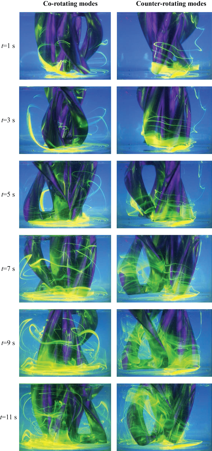
In order to ensure reproducibility of the experiment, the mixing experiment was repeated three times at the apocentric paddle rotating speed of 20 r/min, which proved good reproducibility of the experiment. According to the curve of mixing time, at the same rotating speed, the mixing time in counter-rotating modes was shorter than that in co-rotating modes, especially at low rotating speeds. Taking the rotating speed of 20 r/min as an example, the mixed state of co-rotating and counter-rotating modes at the same t is shown in Figure 4. During mixing process in co-rotating modes, the apocentric paddle pushed the corn syrup at the bottom to the sidewall of the vessel. When reaching the top of the solution level, the corn syrup moved toward the center of the mixing vessel. Apocentric paddle and pericentric paddle drove the corn syrup to move toward the bottom of the vessel and finally achieved uniform mixing. During mixing process in counter-rotating modes, the paddle blade drove the corn syrup solution to move upward enwinding apocentric paddle and pericentric paddle. When reaching the top of the solution level, corn syrup diffused to the sidewall of the mixing vessel. Apocentric paddle drove the corn syrup to move toward the bottom of the vessel and finally achieved uniform mixing after multiple orbital periods.

Figure 4.

Comparing mixing effects of co-rotating and counter-rotating modes.

Tracer experiment in the flow field

According to the mixing experiment, co-rotating and counter-rotating modes of mixing paddle had different mixing efficiencies at the same rotating speed. In order to clearly observe the flow line disturbances in co-rotating and counter-rotating modes at the rotating speed of 20 r/min, the tracer experiments of Arratia et al. ²³ and Saatdjian et al. ²⁴ were taken as reference and designed a tracer test in the flow field. Glycerin with viscosity µ of 1.1 Pa s and density ρ of 1200 kg/m³ was selected as the test solution in the laboratory at a constant temperature of 24°C. Glycerol solution mixed with 3% fluorescein sodium was used as the tracer. Tracer of 5 mL was injected into the bottom center and bottom sidewall of the vessel. Two UV light sources at a wavelength of 362 nm were fixed at both sides of the vessel. The movement of the tracer in co-rotating and counter-rotating modes was observed and is shown in Figure 5.

Figure 5.

Comparison of tracer experiments in co-rotating and counter-rotating modes.

In co-rotating modes, paddle rotation made the mixture-embracing surface produce a downward axial velocity, which prompted the tracer at the bottom sidewall to move upward along the sidewall. The tracer at the bottom center diffused to the edges of the bottom. The two tracers formed a complete flow line. When the apocentric paddle blades moved close to the tracer at the sidewall of the vessel, the tracer began to enwind the apocentric paddle. When the tracer moved to a narrow space between apocentric paddle and pericentric paddle, the velocity ratio of 2:1 between apocentric paddle and pericentric paddle could cut off the complete flow line of the tracer and produce shearing and folding effects. Afterward, the tracer moved toward the bottom and diffused to the edges of the vessel under the impact of a downward axial velocity produced by the mixture-embracing surface.

In counter-rotating modes, paddle rotation made the mixture-embracing surface produce a upward axial velocity, which made the tracer at the bottom center attach to the blade surface and do spiral upward movement. The tracer at the bottom sidewall did spiral movement toward the bottom center. The two tracers formed a complete flow line. When the tracer enwinding the paddle blade moved to a narrow space between two paddle blades, the flow line of the tracer was cut off, shearing and folding effects were produced. Afterward, the tracer moved toward the top and diffused to the edges of the vessel.

According to the tracer experiments in co-rotating and counter-rotating modes, the tracer in co-rotating modes first moved upward along the sidewall of mixing vessel and then moved downward along the central axis of the vessel. The tracer in counter-rotating modes first moved upward along the central axis of the vessel. Then, it moved downward along the sidewall of mixing vessel.

CFD simulation

The curve of corn syrup concentration M changing with time t can be obtained by means of digital image processing. The trajectory of the tracer in the flow field can be observed via tracer experiments. However, such key parameters as velocity vector and pressure change cannot be obtained through these methods. CFD simulation provided a solution to obtain these key parameters that can be used to quantitatively analyze the reasons causing different mixing efficiencies between co-rotating and counter-rotating modes. ANSYS FLUENT 14.0 was adopted as CFD simulation software. Since the paddle blade had a large number of complex curved surfaces, a hexahedral mesh was used to discretize the computational model. During the solving process, user-defined function (UDF) file was created according to the trajectory of the paddle and described by the macro DEFINE_CG_Motion (name, dt, vel, omega, time, dtime). The mesh of computational domain was updated based on the conservative dynamic mesh flow field computation equation (6). ²⁵ Generalized variable ϕ is applicable to any control volume V moving along the boundary of mixing paddles

$$\begin{array}{cc}\multicolumn{1}{c}{}& \frac{d}{\mathrm{dt}}\underset{V}{\int }\rho \varphi \mathrm{dV}+\underset{\partial V}{\int }\rho \varphi (\overrightarrow{u}-{\overrightarrow{u}}_g)·d\overrightarrow{A}\hfill \\ \multicolumn{1}{c}{}& =\underset{\partial V}{\int }\Gamma \nabla \varphi ·d\overrightarrow{A}+\underset{V}{\int }{S}_{\varphi }\mathrm{dV}\hfill \end{array}$$

(6)

Verification of CFD simulation

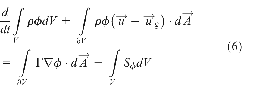
The comparison between experimental results and simulation results is shown in Figure 6. At t = 3 s in co-rotating modes, the tracer was distributed on the positions as shown in Figure 6(a). Apocentric paddle prompted the tracer to move upward along the sidewall of mixing vessel. At t = 3 s, CFD simulation results are shown in Figure 6(b). The tracer in the red box of Figure 6(a) was compared with the flow line in Figure 6(b). It can be seen that they had very similar trajectories. At t = 11 s in counter-rotating modes, the tracer was distributed on the positions as shown in Figure 6(c). The tracer enwinding the apocentric paddle blade moved toward the top of the vessel. At t = 3 s, CFD simulation results are shown in Figure 6(d). The tracer in the red box of Figure 6(c) was compared with the flow line in Figure 6(d). It shows that they had similar trajectories. Meanwhile, in the flow field tracer experiments of co-rotating modes, a vortex flow was formed below the pericentric paddle, as shown in Figure 6(e). The vortex flow was undergoing circular motion following the pericentric paddle. This vortex flow also existed in the simulation result, as shown in Figure 6(f).

Figure 6.

Comparing results of tracer experiment and CFD simulation: (a) t = 3 s in co-rotating modes, (b) t = 3 s in CFD simulation results, (c) t = 11 s in co-rotating modes, (d) t = 11 s in CFD simulation results, (e) a vortex flow below the pericentric paddle, and (f) the CFD simulation results.

As shown in Figure 6, CFD simulation results are in good agreement with the experimental results. Therefore, simulation results were reliable.

Flow line analysis

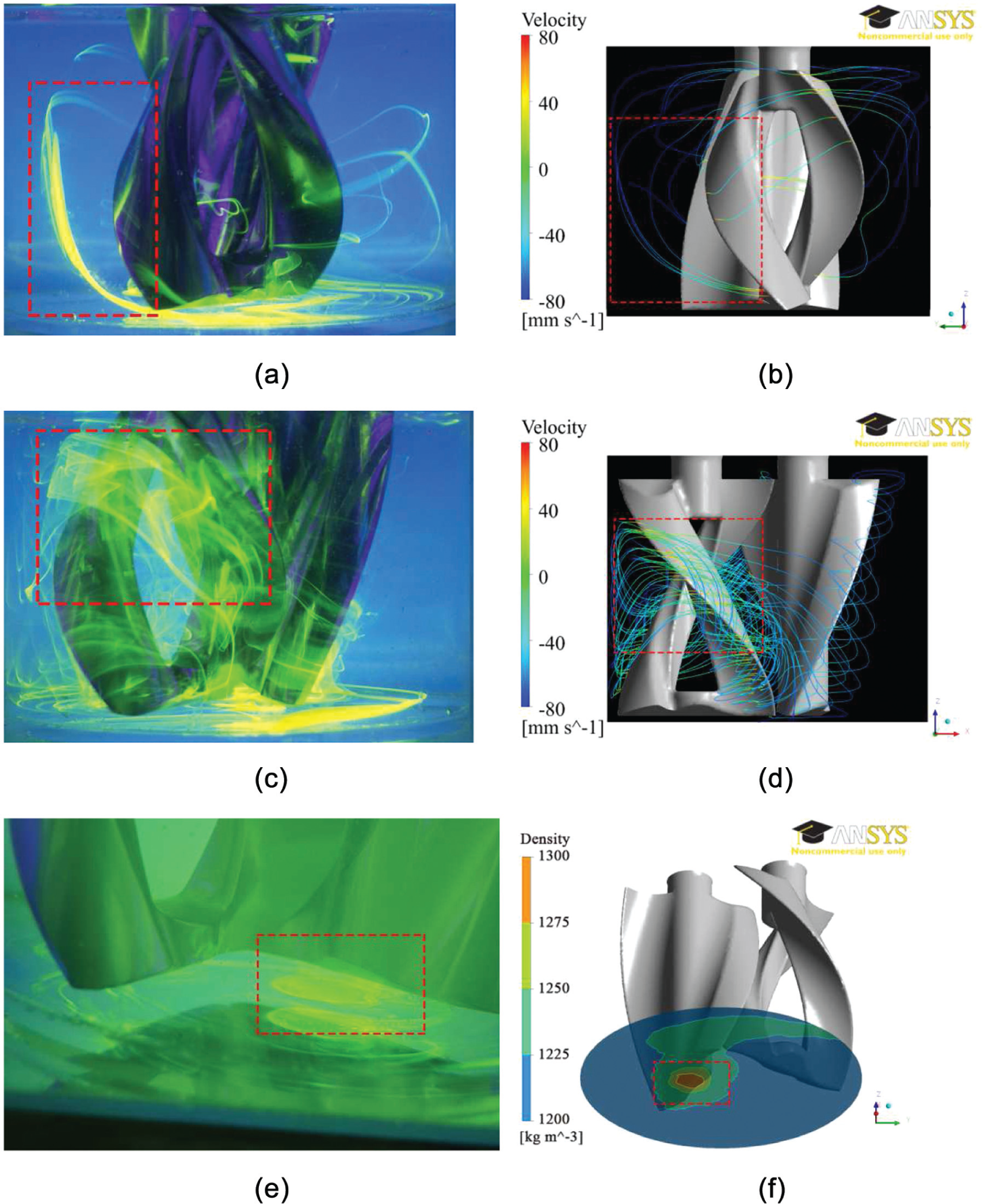
The complete distribution of flow line in the flow field at the rotating speed of 20 r/min obtained from CFD simulation was well consistent with the distribution of the tracer in the experiment. The entire mixing flow field is in the laminar state, where the flow line diffused outward centered on pericentric paddle and apocentric paddle and formed a vortex at the tip of the paddle blade, as shown in Figure 7(a). The rotation of apocentric paddle and pericentric paddle produced a stretching effect on the flow line. As shown in Figure 7(b) and (c), comparing the flow line around the apocentric paddle and pericentric paddle, the maximum flow lines and most obvious stretching effect of flow line occurred around the edge of apocentric paddle. The flow line around pericentric paddle was smoothly distributed, while the flow line around apocentric paddle had more obvious folding phenomenon than that around pericentric paddle. The edges of both paddle blades could cut off the complete flow line, and the flow line between two paddle blades showed squeezed and folded phenomenon, as shown in Figure 7(d).

Figure 7.

(a) Flow line distribution in the Z direction, (b) flow line distribution in the −X direction, (c) flow line distribution in the +X direction, and (d) flow line distribution in the −Y direction.

Research results of Alvarez et al. ⁵ and Shinbrot et al. ²⁶ showed that an effective way to improve mixing efficiency and eliminate IMRs in the laminar flow system was to disrupt the inherent periodic flow and disturb and destroy the stable flow line. In this article, the nonperiodic trajectory of mixing paddle tip could disturb the flow line at any time, disturb the stable circular flow in the laminar flow field, and thereby avoid the formation of IMRs. Research results of Shinbrot et al. ²⁶ and Bresler et al. ¹⁷ showed that stretching, shearing, folding, and chaos effects existed in the laminar flow system. The planetary motion of apocentric paddle and pericentric paddle could produce stretching, shearing, and folding effects on the flow line in the flow field, which is an essential factor causing chaos effects in the laminar flow system.

Flow direction distribution

According to the analysis of flow line in the flow field, the rotational movement of apocentric paddle and pericentric paddle could produce stretching, shearing, and folding effects on the flow line in the flow field. Flow velocity iso-contour can reflect the volume distribution of fluid with the same flow velocity. As shown in Figure 8, flow velocity iso-contour was plotted to analyze the distribution of axial flow, radial flow, and tangential flow in co-rotating and counter-rotating modes, as well as the differences among them.

Figure 8.

(a) Axial velocity iso-contour in co-rotating models, (b) axial velocity iso-contour in counter-rotating models, (c) radial velocity iso-contour in co-rotating models, (d) radial velocity iso-contour in counter-rotating models, (e) tangential velocity iso-contour in co-rotating models, and (f) tangential velocity iso-contour in counter-rotating models.

According to Figure 8(a) and (b), axial flow was mainly distributed on both sides of apocentric paddle tip. Yellow area represents the fluid flowing in the +Z direction at the velocity of 40 mm/s, while light blue area represents the fluid flowing in the −Z direction at the velocity of 40 mm/s. The axial flows on the two sides of apocentric paddle tip showed opposite flow directions. Meanwhile, the axial flows also showed opposite flow directions in co-rotating and counter-rotating modes. Since the autorotation rate of apocentric paddle is twice that of pericentric paddle, radial flow was mainly distributed on both sides of apocentric paddle, as shown in Figure 8(c) and (d). Yellow area represents the fluid flowing in the direction of blade motion at the velocity of 40 mm/s, while light blue area represents the fluid flowing in the opposite direction of blade motion at the velocity of 40 mm/s. It can be seen that radial flow was basically the same in co-rotating and counter-rotating modes. Tangential flow was mainly distributed on the edge of apocentric paddle and along the sidewall near the apocentric paddle, as shown in Figure 8(e) and (f). Light green area represents the fluid flowing in the tangential direction of the blade at the velocity of 10 mm/s, while dark green area represents the fluid flowing in the opposite tangential direction of the blade at the velocity of 10 mm/s. The tangential flow in co-rotating and counter-rotating modes showed opposite directions, but tangential flow had a relatively lower flow velocity.

In summary, both axial flow and radial flow velocities were 40 mm/s, while tangential flow velocity was only 10 mm/s, which was 1/4 of axial flow and radial flow velocities. The flow velocity and direction of radial flow were basically the same in co-rotating and counter-rotating modes, so radial flow had almost no effect on mixing efficiency in co-rotating and counter-rotating modes. Both axial flow and tangential flow had opposite flow directions in co-rotating and counter-rotating modes, but the slow flow velocity of tangential flow had a smaller impact on the mixing efficiency than axial flow. Therefore, it can be inferred that the factors affecting mixing efficiency in co-rotating and counter-rotating modes were in the order of axial flow > tangential flow > radial flow.

Flow velocity distribution

In order to thoroughly analyze the distribution of axial flow velocity and tangential flow velocity in the flow field, in co-rotating modes, five straight lines A1, A2, A3, A4, and A5 were drawn parallel to the Z-axis at 30, 0, and −30 mm of the Y-axis and 60 and −60 mm of the X-axis in Figure 1(a). A total of 20 sampling points were selected from each straight line to plot the distribution curve of axial flow velocity. As shown in Figure 1(b), five straight lines T1, T2, T3, T4, and T5 were drawn parallel to the Y-axis at 50, 25, 0, −25, and −50 mm of the Z-axis. A total of 20 sampling points were selected from each straight line to plot the distribution curve of tangential flow velocity. Since radial flow was almost the same in co-rotating and counter-rotating modes and had little impact on mixing efficiency of mixing experiments, there is no need to separately analyze radial flow. The method for plotting the velocity distribution curve in counter-rotating modes was the same as that in co-rotating modes. It is worth noting that the X-axis in counter-rotating modes was the Y-axis in co-rotating modes, as shown in Figure 9.

Figure 9.

(a) Distribution curve of axial flow velocity, (b) distribution curve of axial flow velocity, (c) distribution curve of tangential flow velocity, and (d) distribution curve of tangential flow velocity.

Comparing the distribution curves of axial flow velocity in co-rotating and counter-rotating modes, both sides of apocentric paddle tip had the maximum axial flow velocity A2 and A4 but in the opposite directions. The velocity curve of A4 was more stable than that of A2, which indicated that the movement of apocentric paddle blade was the main cause of axial flow. The axial flow generated by the interaction between apocentric paddle and pericentric paddle was more than the axial flow generated by the interaction between apocentric paddle and sidewall of mixing vessel. Under the impact of curved surfaces on the paddle, A1 and A3 had axial flows in both +Z direction and −Z direction. Thus, the curve of axial flow velocity passed through the Y-axis twice. Since A5 was far away from the mixing paddle, the flow velocity at this position was relatively slow.

The maximum tangential flow velocity was only 1/4 of the axial flow velocity in co-rotating and counter-rotating modes. But each curve passed through the Y-axis twice, which indicated that the movement of paddle blade produced tangential flows in the opposite directions. The curve had the maximum slope and passed through the origin near the position Y = 0 in co-rotating modes and X = 0 in counter-rotating modes (close to the central axis of the mixing vessel), at the position with shortest distance between curved surfaces of pericentric paddle and apocentric paddle blades, paddle tip T1, and bottom T5. This indicated that the narrow space between two paddle blades had tangential flows in the opposite directions, which can produce a strong shearing effect.

Comparing the velocity distribution in co-rotating and counter-rotating modes, the velocity curves generally showed the same trend but in the opposite directions. In counter-rotating modes, the axial flow in the +Z direction generated between pericentric paddle and apocentric paddle can easily drive the fluid at the bottom of flow field to move upward, produce diffusion effect, and thereby improve the mixing efficiency. In co-rotating modes, the axial flow in the −Z direction generated between pericentric paddle and apocentric paddle drove the fluid at the top of flow field to squeeze downward. Compared with counter-rotating modes, the mixing effect produced by squeezing action was not as obvious as diffusion effect. Thus, it can be inferred that different axial flow direction is the main reason for causing different mixing efficiencies between co-rotating and counter-rotating modes.

Conclusion

This article has combined flow field visualization experiments and CFD simulation to study the impact of double-shaft mixing paddle undergoing planetary motion on the laminar flow mixing system. According to the analysis on tip trajectory of double-shaft mixing paddle undergoing planetary motion, it is predicted that this mixing pattern can effectively inhibit the formation of IMRs in the laminar flow system. Results of mixing experiments showed that IMRs had not emerged in the laminar flow system during the mixing process in both co-rotating and counter-rotating modes. Compared with single-shaft centric mixing paddle or eccentric mixing paddle, double-shaft mixing paddles undergoing planetary motion are more conducive to laminar flow mixing.

Digital image processing was conducted to analyze the mixing efficiency of double-shaft mixing paddle undergoing planetary motion in the laminar flow system. The results showed that the counter-rotating modes of double-shaft mixing paddle undergoing planetary motion had higher mixing efficiency than co-rotating modes, especially at low rotating speeds.

The flow field tracer experiment was carried out to observe the tracer trajectories in co-rotating and counter-rotating modes. The results showed that mixing paddles had a stretching effect on the tracer trajectories in both co-rotating and counter-rotating modes, but the tracer trajectories were in the opposite directions. The tracer flow lines were sheared and folded in the narrow space between apocentric paddle and pericentric paddle.

CFD simulation was adopted to quantify the impact of double-shaft mixing paddle undergoing planetary motion on the flow line and flow direction distribution in the flow field. The results showed that given the same rotating speed, radial flow and tangential flow generated in co-rotating and counter-rotating modes had similar velocity but in the opposite directions, while the velocity and direction of radical flows were approximately the same. It can be inferred from the distribution rule of axial flow, radial flow, and tangential flow in the flow field that axial flow was the main factor affecting the mixing time. The axial flow in the +Z direction generated by counter-rotating modes is more conducive to improve mixing efficiency than the axial flow in the −Z direction generated by co-rotating modes.