Investigation into dynamic response of a three-point bend specimen in a Hopkinson bar loaded fracture test using numerical methods

Abstract

Dynamic fracture toughness of engineering materials at loading rates greater than ${10}^6\mathrm{MPa}\sqrt{\mathrm{m}/\mathrm{s}}$ is widely investigated using the modified Hopkinson pressure bar apparatus. For accurate measurement of dynamic fracture toughness, it is essential to thoroughly understand the dynamic effects excited by the stress wave, such as stress wave propagation characteristics in bars/cracked specimen, the contact situation between the specimen and loading point or supports, and the dynamic response of the fracture specimen. In this work, full transient dynamic analysis techniques are used to comprehend “loss of contact” situation of cracked fracture specimen with an incident bar (impactor) and a transmission bar (supports) in a Hopkinson bar loaded two-bar/three-point bend test. A modified Hopkinson bar loaded experimental setup, including striker, incident, and transmission bars and three-point bend fracture specimen, is modeled using the commercial software ANSYS. The dynamic responses of the specimens made of titanium alloy, high-strength steel, and aluminum alloy are analyzed, and the specimen contact states with the incident and transmission bars are investigated using stress state contours of the specimen along with nodal displacement of the specimen and the bars. The dynamic fracture toughness values for the three specimens are also calculated and compared with the experimental results. The simulation results from the current two-bar/three-point bend test indicated that no “loss of contact” occurs during the first load duration as is previously proved experimentally.

Introduction

Dynamic fracture toughness of engineering materials is an important parameter in damage evaluation and safety assessment of the structures that are often subjected to dynamic loading. The experimental technique currently available for measuring dynamic fracture toughness under a loading rate of $~{10}^6\mathrm{MPa}\sqrt{\mathrm{m}/\mathrm{s}}$ is the Hopkinson pressure bar loading experimental technique. ¹ The reliability of dynamic fracture properties measured by this experimental technique is related to some fundamental dynamic effects, that is, stress wave propagation in bars/specimen, stress state equilibrium in the pre-cracked fracture specimen, and the contact situation of the specimen with the impactor and the supports during loading. A full understanding of these effects is essential before measuring the dynamic fracture toughness using this stress wave loading experimental technique.

Among these fundamental issues associated with the stress wave effect, the contact state of the fracture specimen with impactor and supports is important. It is well known that in three-point bend fracture tests, the cracked sample is initially in contact with the incident bar and supports, while the specimen may lose the contact with incident bar or supports during loading due to strong inertial effect. It should be recognized that once “loss of contact” occurs, whether the specimen loses its contact with the incident bar or with the supports, the fracture mechanics theory derived from the three-point bend test will no longer be effective, and the results calculated will be erroneous. ¹ However, the stress state equilibrium will also no longer exist, and as a result, the formulas for calculating load, displacement, and dynamic fracture toughness will also become invalid. It is therefore essential to thoroughly investigate the contact situation of the specimen during the loading, practically at the moment of the crack initiation.

A “loss of contact” phenomenon was first observed by Böhme and Kalthoff ² in a drop-weight test. They employed strain gauge and opto-electric clip gauge for observing the relative motion of sample with respect to the anvil and found that the travel time of the stress wave from sample loading point to the anvil was greater than the normally required time, implying that “loss of contact” had occurred between the sample and anvil. Kalthoff ³ analyzed the influence of dynamic effects on the procedures of dynamic fracture toughness measurement and suggested that dynamic fracture properties with less error can only be obtained from procedures having no dynamic effects. The researchers^4,5 also thoroughly investigated the “loss of contact” phenomena in Charpy impact tests and suggested that strong inertial effects caused by the specimen’s dimensions and the overhangs result in the “loss of contact” phenomena. Marur ⁶ analyzed Charpy specimens with the help of beam theory and described that the Charpy specimen loading takes place in two steps, that is, first, no contact and second, constrained phase. Marur et al. ⁷ also prepared a simple one-dimensional inertial model of notched beams under impact that also included contact stiffness and contact forces for three-point bend specimens. It is clear that a good deal of work has been undertaken to investigate the “loss of contact” phenomena in the drop-weight and Charpy impact tests, and it is concluded that the “loss of contact” is affected by strong inertial effects. Because of different loading arrangements and loading methods, the knowledge for “loss of contact” phenomena gained from drop-weight and Charpy impact tests is not applicable to Hopkinson bar loaded fracture testing.

In Hopkinson bar loaded three-bar (one incident bar and two transmission bars as supports)/three-point fracture test, Yokoyama and Kishida ⁸ are the first researchers who observed the “loss of contact” phenomena occurring between the incident bar and specimen as well as between the supports and specimen. They pointed out that the “loss of contact” phenomena occurred due to the bending vibrations of the specimen. On the contrary, the experimental work done by Popelar et al. ⁹ indicated that no “loss of contact” occurred between supports and specimen in a one-bar/three-point bend fracture test. Rubio et al. ¹⁰ performed a full two-dimensional (2D) numerical analysis of a one-bar/three-point bend fracture test. The node displacement of the specimen and incident bar in contact was used to describe the “’loss of contact” phenomena. Their results revealed that “loss of contact” occurs between the incident bar and specimen as well as between the supports and specimen at different time intervals. Rittel et al. ¹¹ experimentally observed specimen response in a one-bar/one-point impact test with the help of high-speed photography. Their experimental observation demonstrated that the specimen remains in contact with the incident bar before the specimen “take off.” Guo et al. ¹² experimentally investigated the specimen size effect on contact state and found that the dimensions of specimen and span are important factors that affect specimen’s contact state during loading. Two of the current authors, Jiang and Vecchio, ¹³ experimentally investigated the dynamic effects in two-bar/three-point bend fracture test. In their work, the contact situation at Interface I (contact between incident bar and specimen) and Interface II (contact between supports and specimen) was monitored by a high-speed camera, and the voltage variation of Interfaces I and II was measured using a simple circuit. The results from high-speed photography and voltage variation were coincident and indicated that for the first loading duration, the specimen remained in contact with the incident bar and supports, that is, no “loss of contact” was observed. Until now, it was concluded from previous experimental works^9,11,13 that no “loss of contact” occurred between specimen and supports, while some numerical investigations demonstrated that “loss of contact” occurred. ¹⁰ In order to figure out these contradicting experimental and numerical results, it is necessary to further investigate the “loss of contact” phenomena using numerical simulations and experimental techniques.

The objective of this work is to experimentally verify the previously obtained results, that is, regarding the contact situation of the fracture specimen with impactor and supports using numerical simulation (full transient dynamic analysis technique). To this end, an entire modified Hopkinson pressure bar loaded one-bar/three-point bend fracture experimental setup is modeled and analyzed with the commercial code ANSYS. Specimens made of three different materials, that is, Ti-6-22-22 alloy, high-strength steel, and Al-6061-T6 alloy, are used in the current investigation. The load as a function of time is simulated using a transient dynamic analysis technique, and the specimen stress state contours and the specimen nodal displacement in contact with incident and transmission bars are also analyzed numerically. In addition to analyzing the specimen contact state, the current simulation technique is also used for calculating the dynamic fracture toughness values. The organization of this work is as follows: first, the finite element (FE) analysis technique is introduced in detail, which includes a description of the technique, modeling, meshing, application of initial boundary conditions, and simulation. Then, the simulated results are given in the form of stress, strain, and displacement versus time plots. Also, the stress condition in the model is described with stress contours. Conclusions are drawn related to the “loss of contact” occurring in the Hopkinson bar bend fracture tests. In the end, the dynamic fracture toughness values for the three materials are calculated with the help of crack mouth opening displacement (CMOD) values.

FE analysis

Two-bar/three-point bend fracture setup

The general arrangement and dimensions for the experimental setup and specimen are shown in Figure 1, which primarily consists of a gas gun, a projectile, an incident bar, a transmission bar, and a computer controlled high frequency data acquisition system. The dimensions of the incident and transmission bars are both 38 mm (diameter) × 1524 mm (length), and the dimensions of the striker bar are 38 mm (diameter) × 457 mm (length). The striker, incident, and transmission bars are made of commercial 6061 aluminum alloy. The loading pins are made of high-strength steel having dimensions of 9.5 mm (diameter) × 38 mm (length) located at the end of the transmission and incident bars, as shown in Figure 1. The three-point bend specimens having dimensions of 6.5 mm (width) × 4 mm (thickness) × 40 mm (length), a crack length-to-width ratio of ∼0.5, and a span of 26 mm are used in the simulations.

Figure 1.

Close view of the Hopkinson bar loaded two-bar/three-point bend fracture testing system, including cracked three-point bend fracture specimen arrangement.

Transient FE analysis technique and modeling

The time-varying response of a structure is comprehensively observed by the transient dynamic analysis technique. While performing the transient dynamic analysis in ANSYS, according to the method of solution, the nonlinearities (i.e. large deformation, plasticity and contact, etc.) can be included. The equation of motion for the transient dynamic analysis is the same as the general equation of motion

$$[M]\{\stackrel{··}{u}\}+[C]\{\stackrel{·}{u}\}+[K]\{u\}=[F\{t\}]$$

(1)

where [M] is the mass matrix, [C] is the damping matrix, [K] is the stiffness matrix, and [F{t}] is the load vector.

Equation (1) represents the most general form of dynamic analysis equation with arbitrary time-based loading. Here, the equation of motion is solved using the Newmark time integration scheme. Important in the time integration scheme is the integration time step. In order to determine the nonlinear response, wave propagation effect, and response frequency, the integration time step size should be small. Full matrices with all nonlinearities allowed for [K], [C], and [M] are used while using the full method.

A complete model of the modified Hopkinson pressure bar loaded two-bar/three-point bend fracture experimental setup, including striker, incident and transmission bars, loading pin, three-point bend specimen, and supports, is analyzed using a three-dimensional (3D) full transient dynamic analysis technique. The analysis is performed with ramped loading and the full transient dynamic analysis option. The load is applied in two sub-steps with the first load step to establish the initial boundary condition, and with the ramped loading option, the second load step is ramped from the first load step. The response of the system is observed using the time-history postprocessor. Nodes at crack tip, tip of incident bar, and nodes of specimen in contact points with transmission bar are used to obtain Von Mises stress, strain, and nodal displacement. The transient dynamic analysis technique is complex and requires more computing time. In order to reduce the time for calculation, a half model of the striker and incident bars is used, and an axisymmetric boundary condition is applied in this work. A complete model of the Hopkinson bar setup and three-point bend specimen modeled using the ANSYS software is shown in Figure 2.

Figure 2.

Complete model of the modified Hopkinson pressure bar loaded fracture experimental setup and cracked three-point bend fracture specimen.

Meshing

The meshing of components is done using plane-183 and solid-186 elements. Plane-183 is a higher order 2D, 8-node element with quadratic displacement behavior, best suited for irregular mesh generation. Solid-186 is a higher order 20-node, 3D solid element having quadratic displacement behavior. Each node of this element has 3 degrees of freedom (i.e. nodal x, y, and z direction translations). The element also has hyper-elasticity, large strain, plasticity, and large deflection capabilities, and it is suitable for simulating fully incompressible elastic–plastic materials. The contact between components is defined with element types of target-170 and contact-174. The contact-174 with position on surface finds its application sliding between 3D target deformable surfaces and coupled field contact analyses. For the representation of 3D target surfaces, target-170 is used in this work.

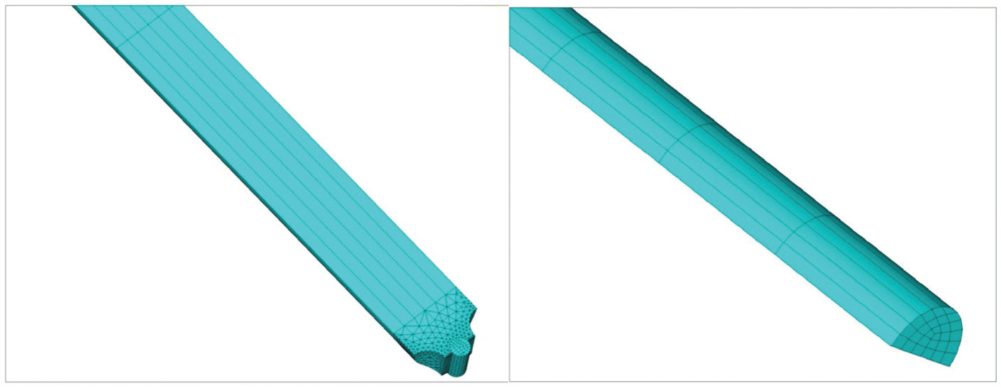
The section of the striker bar is regular and is therefore easily map meshed. Due to the irregular geometry of the incident and transmission bar ends, these are much more difficult to map mesh. Free meshing will increase the number of irregular shape elements and computing time. In order to avoid these problems, the model of the incident and transmission bars is divided into subsections with the major portion map meshed. The presence of the crack in the specimen also makes it difficult for map meshing. One area of the specimen is Quad-map meshed and then extruded to the volume. The meshed model of the incident bar, transmission bar, cracked specimen, and pins is shown in Figures 3 and 4, and the mesh details of each component are given in Table 1.

Figure 3.

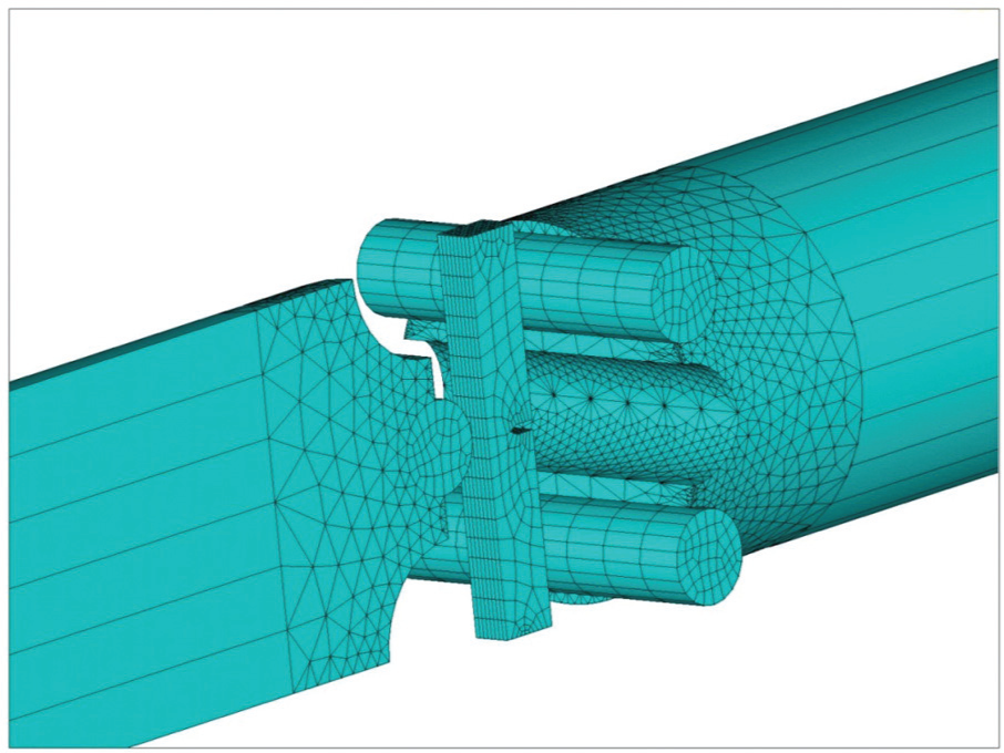
Meshed model of incident and transmission bars, loading pins, three-point bend fracture specimen, and supports.

Figure 4.

Mesh details of incident and striker bars (projectile).

Table 1.

Mesh details of components.

Component	Nodes	Elements
Striker bar	1196	330
Incident bar	11,904	16,514
Transmission bar	40,088	26,878
Specimen	5644	951
Total	58,832	44,673

The transient dynamic analysis is a complicated technique and requires much more computing time compared to quasi-static analysis. When using irregular mesh for the components, the number of elements with violating shape error is greater, and the computing time for the transient dynamic technique increases many times. Whereas the mapped meshing technique is of great help in overcoming all problems associated with element shape violation and increased calculating time and gives a more accurate simulation of the system behavior.

Material model/initial boundary condition

Three different materials, high-strength steel, Ti-6-22-22 alloy, and Al-6061-T6 alloy, are used to machine three-point bend fracture specimens. The projectile, incident, and transmission bars are made of Al-6061-T6 alloy, whereas loading pins are made of high-strength steel. These materials represent different fracture behaviors and elastic–plastic responses. The mechanical properties of these three materials are given in Table 2. The ductile plasticity and damage behavior of the material are incorporated using the power hardening law and the Gurson–Tvergaard–Needleman (GTN)^14,15 model. When the damage and plasticity phenomena occur, the metal voids undergo the micro-mechanical process of growth, nucleation, and coalescence. The material yielding is defined by equation (2)

$$\Phi ={\left(\frac{q}{{\sigma }_y}\right)}^2+2f^{*}{q}_1\cosh \left(\frac{3q_{2}p}{2{\sigma }_y}\right)-\left(1+q_3{f}^{*2}\right)=0$$

(2)

where σ_y is the material yield strength; q is the equivalent stress; p is the pressure; q₁, q₂, and q₃ are the GTN constants; and f^* is the GTN function that is defined by equation (3)

$$f^{*}(f)=\left\{\begin{array}{cc}\hfill f\hfill & \hfill \mathrm{if}\le f_c\hfill \\ \multicolumn{1}{c}{f_c+\frac{\frac{1}{q_1}-f_c}{f_F-f_c}(f-f_c)}& \hfill \mathrm{if}>f_c\hfill \end{array}\right\}$$

(3)

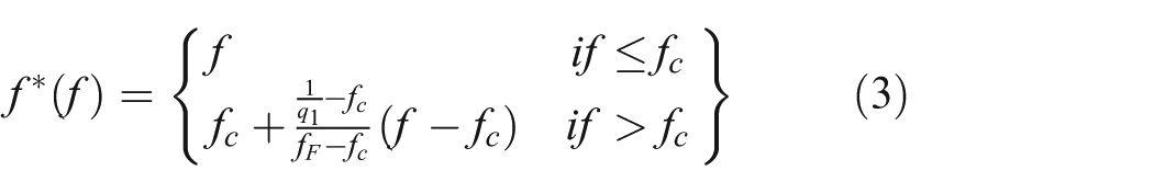
where f_c and f_F are the critical and failure porosity values, respectively. The void nucleation process is substituted in the material model by taking the initial porosity (void volume fraction) “f₀” as 0.04. The other material model parameters considered for the current simulation work are f_n (void nucleation) = 0.04, ε_n (nucleation mean strain) = 0.3, and S_n (standard deviation of mean strain nucleation) = 0.1. For nonlinear isotropic hardening, the power hardening law developed is given in equation (4)

$$\frac{{\sigma }_y}{{\sigma }_o}={(\frac{{\sigma }_y}{{\sigma }_o}+\frac{3G}{{\sigma }_o}{\overline{\in }}^p)}^N$$

(4)

where σ_y is the current yield strength, σ₀ is the initial yield strength, G is the shear modulus, and ${\overline{\in }}^p$ is the microscopic equivalent plastic strain.

Table 2.

Mechanical properties of three materials.

Materials	Tensile yield strength (MPa)	Ultimate tensile strength (MPa)	Poisson’s ratio	Modulus of elasticity (GPa)	Density (kg/m3)
Steel	985	1026	0.3	210	7850
Al-6061-T6 alloy	276	310	0.32	69	2700
Ti-6-22-22 alloy	1164	1220	0.33	114	4510

Whenever we have more than one component in a simulation, for transmission of loads between components we need to define the contacts between components. In the present simulation, the contacts at the interface of the striker with the incident bar, the incident bar with the specimen interface, and the specimen with the transmission bar interface are modeled in the ANSYS software. The displacement constraints are applied to the transmission bar, and specimen is loaded with a loading rate of ${10}^6\mathrm{MPa}\sqrt{\mathrm{m}/\mathrm{s}}$ applied at the nodes of the striker. As a result, the striker moves toward the incident bar. When the striker hits the end of the incident bar, the incident and reflected pulses are generated in the bars and specimen. A constant loading rate is critical in the understanding of material dynamic fracture properties and achievement of constant stress and strain values at the crack tip. It is difficult to calculate an error-free dynamic fracture toughness value in the presence of varying stress and strain values near the crack tip. In the current simulation, constant loading rate of ${10}^6\mathrm{MPa}\sqrt{\mathrm{m}/\mathrm{s}}$ is achieved by modeling and defining accurate contacts between the assembly components.

Determination of “loss of contact”

As mentioned previously, the “loss of contact” is experimentally studied with the help of strain gauges, voltage measurements, and high-speed photography, ¹³ and the “loss of contact” is also investigated numerically with the help of nodal displacement. ¹⁰ In the current numerical investigation, the contact state between the components is determined with the help of dual concepts of both nodal displacements and stress contours in the specimen. The stress and strain values are used to describe the situation of the load at the crack tip, and the corresponding variation of the nodal displacement indicates the contact of the specimen with the incident and transmission bars.

It should be recognized that because of the relative movement of the incident bar and specimen, the contact situation between the incident bar and specimen is more complicated compared to that between the specimen and transmission bar. Therefore, the contact state investigation at this end requires monitoring of the node displacement of incident bar and specimen. The node displacements in contact are taken and the relative difference in node displacement is plotted to analyze the contact state. The contact situation between transmission bar and specimen is monitored from the nodal displacement for specimen in contact with transmission bar. The stress contour movement in the specimen over the loading range can also help in determining the “loss of contact” phenomena.

Results and analysis

Results from high-strength steel specimen

For whole loading cycle, ANSYS time-history command is used to analyze the global response of the system, as well as the variations of stress, strain, and nodal displacement of the specimen. The simulation results of the three-point bend specimen of high-strength steel are shown in Figures 5–7. The variations of Von Mises stress and strain at the crack tip as a function of time are shown in Figure 5(a) and (b). As can be seen in Figure 5(a), the stress value at the crack tip starts increasing at the time of ∼16 μs and then rapidly reaches the peak value of ∼990 MPa that is close to the yield stress. After the maximum value, the stress then drops to a nearly constant stress level of ∼900 MPa. It is found from the careful analysis of the stress versus time, as shown in Figure 5(a), that the rise time and drop time of the stress are quite short (∼2 and 2.5 μs, respectively) as marked in Figure 5(a). The time from the start of the loading to achieving a constant stress is therefore ∼4.5 μs (the sum of rise and drop times), which is almost identical with the transient time of ∼4.7 μs that is determined by the propagation path from the loading point to the supports, using the transverse stress wave velocity (∼3100 m/s) in steel. This result indicates that the transverse stress wave has reached the supports from the loading point in this short period of ∼4.5 μs and then maintained for the entire loading duration. The total loading period for the high-strength steel specimen, determined from the stress versus time and displacement versus time curves, is ∼69 μs, as marked in Figure 5(a). However, from the variation of the crack tip stress as a function of time, it is hard to determine whether the specimen is in a three-point loading state; although the specimen is only loaded in one-point or two-point impact loading, the stress variation may also show similar characteristics of the loading and unloading. Figure 5(b) shows the crack tip strain variation features under a given stress state as shown in Figure 5(a). Clearly, the characteristics of the strain variation in its starting points of loading and unloading, rise time, drop time, and loading duration are exactly the same with stress variation as shown in Figure 5(a).

Figure 5.

High-strength steel specimen: (a) variation of Von Mises stress as a function of time and (b) strain variation as a function of time.

Figure 6.

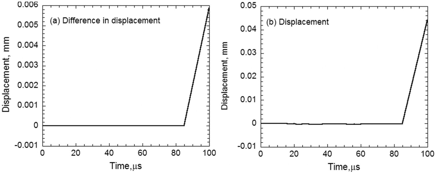
High-strength steel specimen: (a) difference in nodal displacement in contact with specimen and incident bar and (b) node displacement of specimen in contact with transmission bar.

Figure 7.

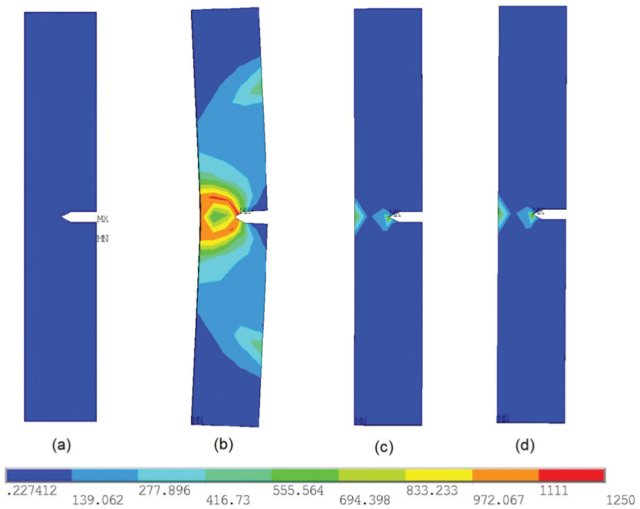
Stress state in high-strength steel specimen at (a) 16 μs, (b) 18 μs, (c) 22.5 μs, and (d) 85 μs, indicating the three-point bend specimen contact situation with loading apparatus and the stress scale bar indicating the levels of stress in the specimen.

Difference in displacement of nodes at the interface of the incident bar and specimen is used to determine the contact state. Here, the difference in displacement is defined as the displacement of node of incident bar subtracted from the displacement of node of specimen. Difference in node displacement of the incident bar and specimen is shown in Figure 6(a). The three-point bend condition requires the specimen to remain in contact with the supports and have minimum values for displacement; therefore, only the displacement of node of specimen in contact with the supports is used for determining the contact state at this end. As can be seen in Figure 6(a), no deviation is found during the loading prior to the unloading point, that is, ∼85 μs as shown in Figure 5(a) and (b). This result indicated that node displacements of the specimen and impactor (incident bar) are the same. The specimen remains in contact with the impactor, that is to say, no “loss of contact” occurred in the interface between the impactor and the specimen. After ∼85 μs, that is, beyond the first loading period of ∼69 μs, the difference in node displacements between the impactor and the specimen increases with increasing time, indicating that the specimen loses contact with the impactor after the first loading period. The variation of the node displacement in contact between the specimen and the transmission bar as a function of time is shown in Figure 6(b); similar conclusion can be drawn that no “loss of contact” occurs within the first loading duration.

To further investigate the specimen contact state with the incident and transmission bars, the stress state contours in the three-point bend specimen at various loading times are analyzed as shown in Figure 7. The stress scale bar is also provided for the indication of stress levels in the different areas of the specimen. The specimen stress state before dynamic loading starts (i.e. 16 μs) is shown in Figure 7(a). After a short time period of 4.5 μs, the stress wave propagates in the specimen, and the stress contours are seen scattered as shown in Figure 7(b), but are symmetric throughout the specimen, indicating that dynamic loading of specimen has begun. Figure 7(c) and (d) shows the stress distribution characteristics in the specimen after the stress wave reaches the supports, at times of 22.5 and 85 μs into loading. Clearly, the stress contours indicate that in most of the specimen area, the stress values are in the range of ∼0.258 to ∼130 MPa, and the stress concentration is observed near the crack tip (as shown in Figure 7(c) and (d)). This suggests that throughout the loading duration, prior to 85 μs, the fracture sample is loaded by the stress wave, and the three-point bend test condition holds (i.e. no “loss of contact” occurred between specimen and bars).

Combining the investigation into the variations of the crack stress, strain, displacement, and stress state contours, it can be concluded that the bend specimen is loaded throughout the first loading period, and the specimen is in a continuous three-point bend loading state (i.e. no “loss of contact” occurred either between the incident bar and specimen or between the specimen and the transmission bar).

Results from Al-6061-T6 specimen

Keeping the same loading/boundary conditions, a simulation is performed for Al-6061-T6 alloy specimens for 200 μs. The stress and strain plots for Al-6061-T6 are shown in Figure 8(a) and (b), and we observe much lower stress variation throughout the loading duration, and the stress propagation time is also found to be ∼4.5 μs. The overall trend for the plots is similar to the high-strength steel specimen, except that the load duration measured is longer, that is, ∼163 μs. As previously discussed, in order to determine the contact situation of the specimen with the incident bar, the difference in displacement for two nodes is plotted in Figure 9(a). Displacement of the node in contact with the transmission bar is plotted in Figure 9(b). For the entire loading duration of 163 μs, the same conclusion that three-point bend loading condition remains valid is drawn. The stress contours for the specimen along with the stress scale bar are shown in Figure 10. It is noted that the stress wave just reaches the intact face of the specimen (interface between the impactor and the specimen) at 22 μs, and the specimen starts loading at this time as shown in Figure 10(a). At 25 μs, the stress wave passes through the specimen and the specimen is loaded, and the stress contours are therefore seen as shown in Figure 10(b). At 26.5 μs, when the stress wave reaches the supports, the stress concentration is observed at the crack tip, and this stress concentration continues for the entire loading duration (i.e. 163 μs), indicating that the three-point bend specimen condition remains valid throughout the loading duration, which is the same conclusion as previously determined for the high-strength steel specimen.

Figure 8.

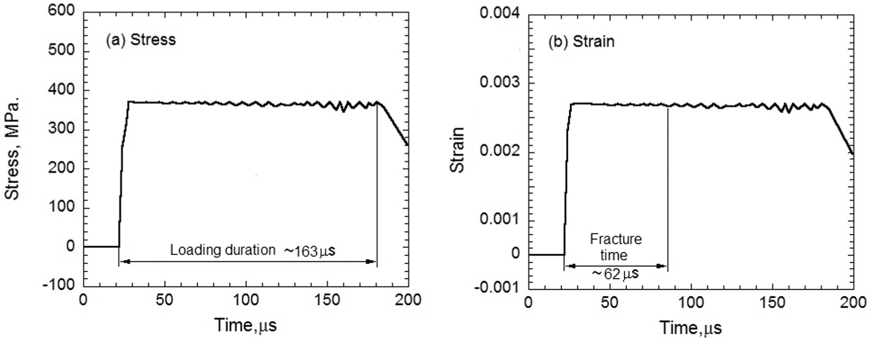
Al-6061-T6 specimen: (a) variation of Von Mises stress variation as a function of time and (b) strain variation as a function of time.

Figure 9.

Al-6061-T6 specimen: (a) difference in nodal displacement in contact with the specimen and the incident bar and (b) node displacement of specimen in contact with the transmission bar.

Figure 10.

Stress state in Al-6061-T6 specimen at (a) 22 μs, (b) 25 μs, (c) 26.5 μs, and (d) 185 μs, indicating the three-point bend specimen contact situation with loading apparatus and the stress scale bar indicating the levels of stress in the specimen.

Results from Ti-6-22-22 alloy specimen

The variations of stress, strain, and nodal displacement of the Ti-6-22-22 alloy specimen are shown in Figures 11 and 12, respectively. A similar behavior to previously examined specimens is found in this high-yield-strength specimen. The time for the stress wave to propagate through the specimen is also 4.5 μs for Ti-6-22-22 alloy specimen, but the loading duration for this specimen is the shortest, that is, ∼ 51 μs. In order to examine the three-point bend specimen state, for the entire loading duration, the stress contours are also given in Figure 13. It is noted that the specimen loading starts at 16 μs as shown in Figure 13(a). At 18 μs, the stress contours are observed as shown in Figure 13(b). At this time, the stress at the crack tip reaches a maximum as shown in Figure 11(a). After 4.5 μs, when the stress wave reaches the supports, a stabilization of stress is observed, and the stress concentration is seen at the crack tip as shown in Figure 13(c). As shown in Figure 13(d), at 67 μs, the same stress contours pattern as that at 22.5 μs is observed, suggesting that the three-point bend loading condition holds throughout the loading period. The analysis of plots for displacement and stress contours for the Ti-6-22-22 alloy specimen also indicates that for the entire loading duration (i.e. 51 μs), the specimen remains in contact with the loading apparatus and “loss of contact” is only seen after the first loading period.

Figure 11.

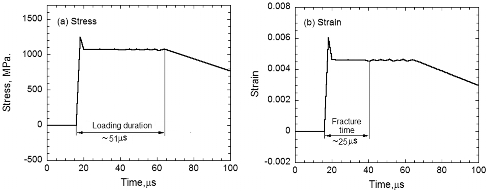
Ti-6-22-22 alloy specimen: (a) variation of Von Mises stress at the crack tip as a function of time and (b) strain variation as a function of time.

Figure 12.

Ti-6-22-22 alloy specimen: (a) difference in nodal displacement in contact for specimen and incident bar and (b) node displacement of specimen in contact with transmission bar.

Figure 13.

Stress state in Ti-6-22-22 alloy specimen at (a) 16 μs, (b) 18 μs, (c) 22.5 μs, and (d) 67 μs, indicating the three-point bend specimen contact situation with loading apparatus and the stress bar indicating the levels of stress in the specimen.

Dynamic fracture toughness calculation

The dynamic fracture toughness is the most important material dynamic fracture property. A valid three-point bend specimen contact state is necessary for the accurate calculation of the dynamic fracture toughness. It is also important to mention that the actual material fracture behavior cannot be simulated by only considering elastic–plastic models. For the actual simulation of crack behavior, the micro-mechanical material properties need to be considered. In this work, the micro-mechanical crack propagation behavior due to void coalescence and nucleation is incorporated by considering the GTN material model. The voids nucleation takes place at the interface of the inclusions with the metal matrix and usually exhibits elastic–brittle response. The damage mechanism is also initiated by the weak-bonded metal matrix particles. The formation and propagation of macroscopic crack are linked with the micro-mechanical behavior of the metal matrix voids. Hence, the micro-mechanical properties are very important in the accurate calculation of dynamic fracture toughness. The dynamic fracture toughness is defined by a well-known relationship given in equation (5)

$$K_{\mathrm{Id}}=K_I(t_f)$$

(5)

where K_Id is the dynamic fracture toughness, K_I is the stress intensity factor, and t_f is the time of fracture. The calculation of dynamic fracture toughness is dependent on fracture time and the stress intensity factor value at the time of fracture. The accurate calculation of dynamic fracture toughness value is strongly dependent on the specimen stress equilibrium and the contact state during loading. After analyzing the specimen contact situation during loading in detail, the dynamic fracture toughness values for the three materials tested are calculated numerically and compared with the experimental results. In the current simulation work, the time for fracture is determined from the drop in the strain values at the crack tip as indicated in Figure 5(b). For the numerical dynamic fracture toughness calculation, the CMOD value at the time of fracture for a three-point bend specimen is evaluated and substituted into equation (6) ¹⁶ with an assumption that static conditions are valid for dynamic case

$$K_I(t)=\frac{E*\mathrm{CMOD}}{4\sqrt{a\alpha }}\frac{k_{\beta }(\alpha )}{{\nu }_{\beta }(\alpha )}$$

(6)

where “α” is the ratio of crack length, a, to specimen width, W, and “β” is the ratio of specimen span, S, to specimen width, W. $k_{\beta }(\alpha )$ and $v_{\beta }(\alpha )$ are the non-dimensional functions. The CMOD values for the three materials from loading point to the fracture time are plotted in Figure 14.

Figure 14.

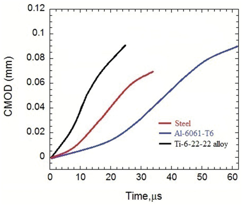
CMOD value plot for steel, Al-6061-T6 alloy, and Ti-6-22-22 alloy.

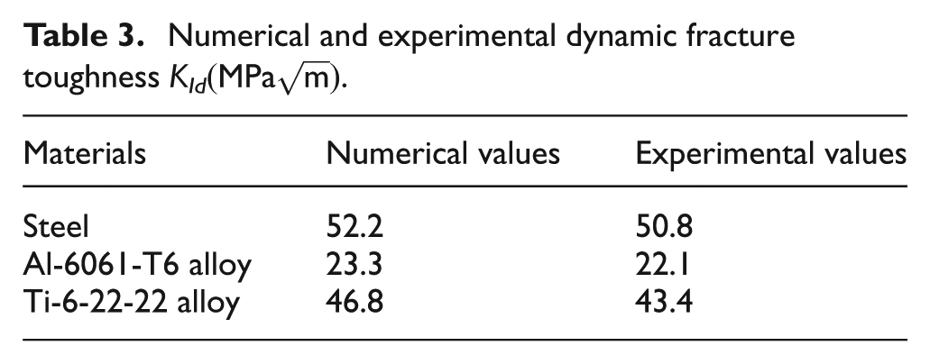
The fracture time, a necessary parameter, is detected by a strain gauge technique. ¹ The dynamic fracture toughness, which is the dynamic stress intensity value at the time of fracture, is therefore determined experimentally. The comparison of numerically and experimentally calculated dynamic fracture toughness values is provided in Table 3. The calculated numerical dynamic fracture toughness values are in good agreement with the experimental values.

Table 3.

Numerical and experimental dynamic fracture toughness K_Id $(\mathrm{MPa}\sqrt{\mathrm{m}})$ .

Materials	Numerical values	Experimental values
Steel	52.2	50.8
Al-6061-T6 alloy	23.3	22.1
Ti-6-22-22 alloy	46.8	43.4

Discussion

To analyze the stress wave propagation behavior, it is essential to determine some characterization time parameters, such as transient time (t_p), time to fracture (t_f), and load duration (t_d). After the loading starts, the transient time for the stress wave propagation within the specimen is obtained from rise and drop of yield stress values, as marked in Figure 5(a). After stabilization of stresses at the crack tip, the fracture time for the specimen is obtained from the drop in the strain values as marked in Figure 5(b), and the load duration time is obtained by analyzing the stress, strain, and displacement plots. The stress wave speed (C_T) in the specimen is defined by equation (7) ¹²

$$C_T=\frac{{[(S/2{)}^2+W^2]}^{\frac{1}{2}}}{t_p}$$

(7)

where S and W are the span and the width of the specimen, respectively, and the transient time in the specimen (t_p) is the time required for the stress wave to reach the specimen/support interface from the incident bar/specimen interface. During the initial fracture phase when micro-voids growth and coalescence occur, the variations in the stress and strain values plot at the crack tip shown in Figures 5, 8, and 11 are negligible, and gradually, stress and strain variations start increasing suggesting that the initial fracture phase has ended. During the later fracture phase, the increase in the stress and strain variations indicates rapid material fracture process, and the macro-crack propagation takes place even between the voids.

The load duration (t_d), time to fracture (t_f), transient time for stress wave in specimen (t_p), and stress wave velocity in the specimen, determined numerically, are given in Table 4. The experimental results ¹³ and theoretical value for the stress wave velocity are also given in Table 4 for comparison. It is obvious that the numerically calculated time parameters for transient time, fracture time, and dynamic load duration are in good agreement with the experimental values. Furthermore, the transverse wave velocity calculated from equation (7) in the specimens is ∼3230 m/s, which is almost identical to the theoretical value of the transverse wave speed in the specimen (3111 m/s for the high-strength steel and Al-6061-T6 alloy, and 3100 m/s for the Ti-6-22-22 alloy). These agreements confirm that the FE analysis procedure proposed in this work is reliable and valid, and the conclusion that no “loss of contact” occurred during the first loading period is correct.

Table 4.

Comparison of various time parameters.

Materials	Numerical calculated time (μs)			Numerical wave velocity (CT), m/s	Experimental time (μs)			Experimental wave velocity (CT), m/s
	Transient time (tp)	Fracture time (tf)	Load duration (td)		Transient time (tp)	Fracture time (tf)	Load duration (td)
Steel	4.5	32	69	3230	4.7	34.4	74	3100
Al-6061-T6 alloy	4.5	62	163	3230	4.7	61.6	200	3100
Ti-6-22-22 alloy	4.5	25	51	3230	4.7	28.4	68	3100

As previously discussed, two authors of this work have analyzed this phenomenon in detail using voltage measuring methods, and the results of previous experimental work, as well as current simulation, demonstrate that no “loss of contact” is observed for the specimen, either with the incident or transmission bars during first loading duration. The “loss of contact” may occur after the first loading period, while any “loss of contact” after first loading duration will not have any effect on the dynamic fracture toughness values as the parameters required for its calculation are determined using only valid three-point bend fracture theory, prior to the “loss of contact.” The current simulation technique is also used to calculate the dynamic fracture toughness of the three materials considered. The dynamic fracture toughness values calculated from the current simulation work are in good agreement with the experimentally obtained values.

Conclusion

In this work, a transient dynamic analysis technique is used to investigate the contact situation of specimen with incident and transmission bars in two-bar/three-point bend fracture testing system. An entire experimental setup, including striker bar, incident bar, transmission bar, specimen, and supporting structure, is modeled using the commercial software ANSYS. The load as a function of time is applied using full transient dynamic technique. The transient time, fracture time, and loading period, as well as the transverse stress wave velocity in the specimen, are determined from the current FE analysis. The specimen contact situations with the impactor and supports are investigated using the stress and stain at the crack tip, stress contours, and node displacement. The results from the three specimens of high-strength steel, Al-6061-T6 alloy, and Ti-6-22-22 alloy indicated that no “loss of contact” occurs during the first loading period, as was also experimentally proved previously. The dynamic fracture toughness values calculated from the current simulation are also in good agreement with the experimental values.

The numerical procedure adopted in this work will also be helpful in understanding other dynamic effects like stress wave propagation in specimen/bar and specimen stress equilibrium. There is a need for more simulations to be run in order to comprehend the effects of specimen dimensions, span, and overhangs on specimen dynamic response.