Forward kinematics solutions of a special six-degree-of-freedom parallel manipulator with three limbs

Abstract

This article presents a special 6-degree-of freedom parallel manipulator, and the mechanical structure of this robot has been introduced; with this structure, the kinematic constrain equations are decoupled. Based on this character, the polynomial solutions of the forward kinematics problem are also presented. In this method, the closed-loop kinematic chain of the manipulator is divided into two parts, the solution forward position kinematics is obtained by a first-degree polynomial equation first, and then an eighth-degree polynomial equation in a single variable for the forward orientation kinematics is obtained. Based on those solutions, the configurations of the robot, including position and orientation of the end-effector, are graphically displayed. A numerical simulation is given to verify the algorithm, and the result implies that for a given set of input values, the manipulator can be assembled in eight different configurations at most. And a set of experiments illustrate the motion ability for forward kinematics of the prototype of this manipulator.

Introduction

The various types of mechanisms have been applied in many robotic fields. Nowadays, some parallel mechanisms (PMs) have attracted a lot of attention. PMs have many advantages over serial mechanisms, such as high stiffness, large payload capacity, compact structure, low inertia, and high accuracy. These characteristics allow the parallel robot to be used in various fields. Parallel manipulators can be used as the space docking prototypes, the flight training devices, the vibration and earthquake simulators, the mining products, the tunnel shields, the forging manipulators, assisted surgeries, and so on. ¹

As a significant example of such PMs, Gough and Whitehall ² invented a tire detecting device having 6-degree-of freedom (DOF). Later, Stewart ³ designed the Stewart platform for flight simulation and analyzed kinematics of this platform. Hunt ⁴ termed a class of mechanisms including the Stewart platform as the parallel manipulators. Since then, a large number of PMs have been built and several distinctive design and analysis approaches were introduced in this field. The screw theory^5,6 as an effective tool is used to analyze the motions of mechanisms. The theory of differential geometry^7,8 provided precise mathematical descriptions for the motion characteristics of kinematic joints. The G_F sets^9,10 presented a practical method for analyzing the interaction motion characteristics of the end-effector. Researchers who developed different achievements contributing to the advancement of parallel manipulator are deeply appreciated. However, there are still several problems that need to be further investigated. One of the most difficult tasks of parallel manipulators is finding the suitable solution for the forward kinematics. For a general 6-DOF parallel manipulator, it is well known that the input joint values are used to solve the position and orientation of the end-effector relative to the base platform. The position and orientation of the mobile platform are used to determine the actuated joint values. As we can see that the inverse kinematics of the parallel manipulator is usually simple. Unlike inverse kinematics, the forward kinematics problem leads to a system of highly coupled nonlinear constrained equations; it is hard to solve.

In order to find an efficient algorithm to determine the forward kinematics solutions, some studies on the kinematics have been reported, and many approaches have been proposed in the past. These approaches mainly are categorized into algebraic elimination methods and numerical methods.

Using the algebraic elimination methods, the kinematic constraint equations of the nonlinear equations are converted into a resultant polynomial equation with a single unknown, so that it will bring the closed-form solutions or analytical solutions in solving the polynomial equations. From the multiple solutions of the polynomial, we can get physical insight on the kinematic behavior and obtain exact configurations of the mechanism. Based on the algebraic elimination method, Griffis and Duffy, ¹¹ Innocenti and Parenti-Castelli, ¹² and Nanua et al. ¹³ presented a univariate 16th-degree polynomial equation to this problem. The univariate 20th- and 40th-degree polynomials were obtained in the literatures,^14–16 respectively. Recently, in order to get a unique solution of the polynomial equation, an algebraic elimination method ¹⁷ is proposed which uses reduced Grobner bases and lexicographic ordering to obtain a small size of 14th-degree univariate polynomial.

However, it is worth noting that the degree of the univariate polynomial is usually high by means of algebraic elimination method; in practice, the high degree is more difficult to solve, and to obtain the closed-form solutions or analytical solutions is difficult.

With the development of computer technologies, some new techniques, based on numerical procedure or extra sensor to acquire the forward solutions, are also kinds of effective methods. The numerical methods^18–24 were introduced to overcome this problem, such as Newton–Raphson method, continuation methods, neural networks, genetic algorithms, interval analysis, and alternative approach. Although numerical methods are accurate and can provide unique solution to the forward kinematics problem, the main challenge such as Newton–Raphson method is difficult to ascertain the number of iterations and to select the initial estimation of the task space, while some of these approaches rely on powerful computer hardware.

Moreover, the forward kinematics problems for the low-DOF parallel manipulators are also presented by Bhatti et al. ²⁵ and Zhang and Lei. ²⁶ A closed-form solution has been presented by Zhang et al. ²⁷ for the general 5-5B in-parallel platform.

Although many approaches have been proposed in the forward kinematics problem, much effort still continues to explore more suitable algorithms. Among the above methods, we consider polynomial-based approach to solve the forward kinematics problem of the proposed manipulator, using a pair of tan-half-angular displacements by elimination methods. ²⁸ The advantage of using a univariate polynomial equation is that all the possible solutions can be obtained. ²⁹

In this article, we design a special 6-DOF parallel manipulator with three limbs (TLPM). The literature ³⁰ only introduced the inverse kinematics, and the forward kinematics of this mechanism not involved. However, to get the forward kinematics solutions is essential to the workspace analysis, dexterity evaluation, optimum design, fault restoration, and singular configurations. ³¹ The forward kinematics is also used for the analysis of assembly mode, which is concerned with the number of possible modes of assembly and helps to find optimum configurations. Moreover, to get the solutions of the forward kinematics is necessary for real-time operations. In this project, the solutions for the forward position kinematics (FPK) yield a first-degree polynomial equation in a single variable of the TLPM and obtain an eighth-degree polynomial equation for the forward orientation kinematics (FOK) in a single variable, respectively. The real solutions to the problem can be found for some configurations.

This article is organized as follows: the characteristics of the manipulator and the limb parameters include the mechanism are introduced in section “Proposed manipulator.” The modeling of kinematic equations is addressed in section “Modeling of the TLPM.” Then, the polynomial equations for obtaining the solutions of the positional and orientational variables are presented in section “Forward kinematics solutions.” The results are presented via a set of numerical simulation and experiment in section “Simulation and experiment.” Finally, the conclusions are drawn in section “Conclusion.”

Proposed manipulator

This section presents a special parallel manipulator that was designed by Prof. Gao’s group from Shanghai Jiao Tong University. For the convenience of the analysis, forward kinematics, the structure of the manipulator, and the corresponding parameters will be introduced in this section.

Characteristics of the TLPM

As shown in Figure 1, this TLPM has a parallel kinematic structure with three identical limbs connecting the fixed platform to the moving platform. Each limb is configured by an active revolute (R) joint, two passive R joints, an active prismatic (P) joint, and a universal (U) joint. This design has 6 DOFs, namely, three rotations around x-, y-, and z-axes and three translations along x-, y-, and z-directions. The six active joints are driven by six servo motors and actuator displacements are measured by linear potentiometers. The manipulator is supplied by an alternating current (AC) power source, and six AC–direct current (DC) transformers are used in this system. Advantages of this structure are three main aspects: (1) three translational and three rotational motions are decoupled, the end-effector position is only determined by three lengths of prismatic actuators, while the rotational angles are relative to all six inputs, so that it is easier to compute the end-effector position and orientation of the manipulator in inverse and forward kinematics. (2) The kinematic performances help the system to improve the real-time control capability. (3) Reconfiguration can be easily realized due to the modularized design approach and has a sufficient workspace.

Figure 1.

Initial configuration of the TLPM.

Geometric parameters of the TLPM

Corresponding to the mechanical structure design of the limb in Figure 2(c), each limb has been assembled on the base platform with an angle β₁. The axes of all the R joints and the guide directions of the three P joints intersect at a common point p at the same time.

Figure 2.

Geometric parameters of the TLPM: (a) moving platform, (b) base platform, and (c) single limb.

The ith, i = 1, 2, 3, limb connects the base platform through a universal joint, and q_i, i = 1, 2, 3, denotes the point where the two axes of the U joint intersected at the base platform. Besides, the points q₁, q₂, and q₃ lie evenly on a circle of radius L, and the U joints are tangential to the circular.

In this study, the geometric design parameters of the ith limb are defined by the vector d₁ = [α₁ α₂ β₂] ^T . As shown in Figure 2(c), α₁ denotes the angle between the axis of the R1 joint and the axis of R2 joint; α₂ denotes the angle between the axis of the R2 joint and the axis of the R3 joint; β₂ is defined from the geometric center of line of moving platform to the axis of the R3 joint. Angles η_1i, i = 1, 2, 3, are defined as the angles between the projection of the axes of the actuated P joints on the base platform and a given reference in that plane under the state of initial configuration, as shown in Figure 2(b). And angles η_2i, i = 1, 2, 3, are defined between the projection of axis of the R3 joint of the ith limb on the moving platform and a given reference in that plane, as shown in Figure 2(a). The input parameters θ_i3 and l_i, i = 1, 2, 3, denote the actuator angle and actuator length with respect to the initial values, respectively.

Modeling of the TLPM

The kinematic diagram of the TLPM is illustrated in Figure 3. For the convenient analysis, a moving coordinate system (MCS) is located at the point p and fixed to the moving platform. Its z′-axis is defined as the axis in the direction of the unit vector z ₁₃-and x′-axis is normal to z′-axis in the plane that is defined by vectors z ₂₃ and z ₃₃. A fixed coordinate system (FCS) is fixed to the base platform and its origin always fixed at the initial position of the point p. Its z-axis is defined as the axis in the direction from the o to p and x-axis is parallel to the vector oq ₁ .

Figure 3.

Kinematic diagram of the TLPM.

Now, in order to write the kinematic constraint equations, we defined the vectors u _i , v _i , and w _i , i = 1, 2, 3, along the axes of the ith limb, as shown in Figure 3. And then the vectors v _i and w _i will be expressed in the frame FCS; with these vectors, we will derive kinematic constraint equations in the following situation.

In the view of the mechanical structure of this manipulator, each link has been set up on the base platform with a certain angle, the fixed points q_i, is uniform distribution on the base platform. Therefore, the base of the limb constitutes an equilateral triangle. Here, we denote c as the abbreviation of cosine and s for sine in this article. Referring to Figure 3, the position vector of point q_i with respect to the FCS is expressed as

$${\mathit{q}}_i={\mathit{R}}_{{\eta }_{i1}},(\begin{array}{ccc}L\hfill & 0\hfill & -H\hfill \end{array}{)}^T,i=1,2,3$$

(1)

where

$${\mathit{R}}_{{\eta }_{i1}}=\left[\begin{array}{ccc}\mathrm{c}{\eta }_{i1}\hfill & -\mathrm{s}{\eta }_{i1}\hfill & 0\hfill \\ \multicolumn{1}{c}{\mathrm{s}{\eta }_{i1}}& \mathrm{c}{\eta }_{i1}\hfill & 0\hfill \\ \multicolumn{1}{c}{0}& 0\hfill & 1\hfill \end{array}\right]$$

Since the base platform is an equilateral triangle, the position vectors q _i can be calculated by equation (1), and Cartesian position of the moving platform is denoted as p  = (x, y, z) ^T . There exist at most three lines in the base which satisfy three distances between the point p and the ith U joint is

$$\Vert \mathit{p}-{\mathit{q}}_i\Vert =(l_{i0}+l_i{)}^2,i=1,2,3$$

(2)

where l_0i is the initial length of the limb and l_i is the input length of ith parametric joint.

When the manipulator is at initial position, the projection of z′-axis and x-axis on the base platform is coincidence, and the point p is right above the center of the base platform O and H equals to L. Then the axis of R joints in each limb is pairwise orthogonal; the intersection angle measured from the base platform to the axis of P joint is π/4. The initial length of pq_i is $\sqrt{2}L$ , and every joint variable equals to 0.

We also set a link Cartesian frame (L _ij CF) which is attached to each link of the ith limb i = 1, 2, 3, j = 1, 2, 3. As a consequence, all link coordinate frames used in this article will have their origin at point p. For the frame L _i1CF, which is located at the first link of the ith limb, where the z_i1-axis is defined in the direction from p to q_i, the x_i1-axis is orthogonal to the z_i1-axis and the Y_i-axis, and the direction of the y_i1-axis is determined by the right-hand rule. Where the vectors of the Y_i-axis can be expressed as

$${\overrightarrow{Y}}_i=\mathit{R}(\mathit{z},{\eta }_{i1})\overrightarrow{y},i=1,2,3$$

(3)

where

$$\overrightarrow{y}=(\begin{array}{ccc}0\hfill & 1\hfill & 0\hfill \end{array}{)}^T$$

Then, the vectors from p to q _i are denoted as z _i1, and thus z _i1 can be computed as

$${\overrightarrow{z}}_{i1}={\overrightarrow{q}}_i-\overrightarrow{p},i=1,2,3$$

(4)

and its unit vectors are given by

$${\hat{z}}_{i1}=\frac{{\overrightarrow{q}}_i-\overrightarrow{p}}{\Vert {\overrightarrow{z}}_{i1}\Vert }$$

(5)

The vectors ${\overrightarrow{x}}_{i1}$ are perpendicular to both Y_i-axis and z _i1-axis, which can be computed as

$${\overrightarrow{x}}_{i1}={\overrightarrow{Y}}_i\times {\overrightarrow{z}}_{i1},i=1,2,3$$

(6)

and its unit vectors are given as

$${\hat{x}}_{i1}=\frac{{\overrightarrow{Y}}_i\times {\overrightarrow{z}}_{i1}}{\Vert {\overrightarrow{x}}_{i1}\Vert }$$

(7)

Finally, the vectors y _i1 are perpendicular to both x_i1-axis and z_i1-axis, and the directions are determined by the right-hand rule, which can be computed as

$${\overrightarrow{y}}_{i1}={\overrightarrow{x}}_{i1}\times {\overrightarrow{z}}_{i1},i=1,2,3$$

(8)

and its unit vectors are given as

$${\hat{y}}_{i1}=\frac{{\overrightarrow{x}}_{i1}\times {\overrightarrow{z}}_{i1}}{\Vert {\overrightarrow{y}}_{i1}\Vert }$$

(9)

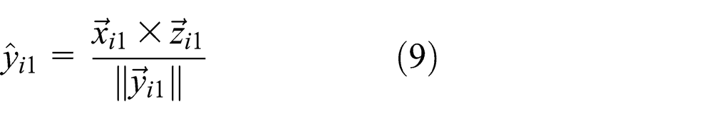
Therefore, in view of the above-mentioned facts, the rotation matrices associated with each limb from the frame L _i1CF to the frame FCS, which are denoted as R _i0, and given as

$${\mathit{R}}_{i0}=[\begin{array}{ccc}{\hat{x}}_{i1}\hfill & {\hat{y}}_{i1}\hfill & {\hat{z}}_{i1}\hfill \end{array}],i=1,2,3$$

(10)

Referring to Figure 3, coordinate frames L _i1CF and L _i2CF are associated with Link1 and Link2 of the ith limb, respectively. The rotation matrices from frame L _i1CF to frame L _i2CF are written as

$${\mathit{R}}_{i1}=\left[\begin{array}{ccc}\mathrm{c}{\theta }_i\hfill & -\mathrm{s}{\theta }_i\mathrm{c}{\alpha }_1\hfill & \mathrm{s}{\theta }_i\mathrm{s}{\alpha }_1\hfill \\ \multicolumn{1}{c}{\mathrm{s}{\theta }_i}& \mathrm{c}{\theta }_i\mathrm{c}{\alpha }_1\hfill & -\mathrm{c}{\theta }_i\mathrm{s}{\alpha }_1\hfill \\ \multicolumn{1}{c}{0}& \mathrm{s}{\alpha }_1\hfill & \mathrm{c}{\alpha }_1\hfill \end{array}\right],i=1,2,3$$

(11)

Now, it is easy to write the expressions of vectors w _i with respect to the frame FCS; thus, substitution of equations (10) and (11) yields

$${\mathit{w}}_i={\mathit{R}}_{i0}{\mathit{R}}_{i1}\mathit{z}$$

(12)

where

$$z=(\begin{array}{ccc}0\hfill & 0\hfill & 1\hfill \end{array}{)}^T$$

For the purpose of expressions of the vectors v _i in frame FCS, we need to express it in frame MCS as ${\mathit{v}\prime }_i$ first, and we get

$${\mathit{v}\prime }_1=\mathit{z}$$

(13)

$${\mathit{v}\prime }_2=[{\begin{array}{ccc}\mathrm{s}{\varphi }_1\hfill & 0\hfill & \mathrm{c}{\varphi }_1]\hfill \end{array}}^T$$

(14)

$${\mathit{v}\prime }_3=[{\begin{array}{ccc}\mathrm{s}\phi \mathrm{s}{\varphi }_2\hfill & \mathrm{s}\phi \hfill & \mathrm{s}\phi \mathrm{c}{\varphi }_2]\hfill \end{array}}^T$$

(15)

where

$$\begin{array}{cc}\multicolumn{1}{c}{{\varphi }_1}& =2\arcsin \left(\frac{\sqrt{3}\sin {\beta }_2}{2}\right)\hfill \\ \multicolumn{1}{c}{{\varphi }_2}& =\frac{{\varphi }_1}{2}\hfill \\ \multicolumn{1}{c}{\phi }& ={\varphi }_1+\arctan \left(\frac{\tan {\beta }_2}{2}\right)\hfill \end{array}$$

In the solution of the forward kinematics problem, the orientation of the end-effector will be expressed by three Euler angles which are noted as α, β, and γ, respectively. If the actuated joint values are known, the corresponding matrices and the initial angles α₀ and γ₀ (they are decided by the lengths of prismatic actuators) can be computed. Therefore, the orientation of reference frame is also determined. As a result, we use the frame L₁₂CF, which is fixed to the second link of the first limb as the reference frame for the definition of the Euler angles. The three Euler angles with the rotation transformed into the frame MCS can be described as follows: the frame L₁₂CF is rotated around z₁₂-axis about an angle α which took x₁₂-axis in the plane defined by vectors w ₁ and v ₁, the latter coordinate system is rotated around y′₁₂-axis by the angle β to take z₁₂-axis in coincidence with z′-axis, and then the rotation of new coordinate is rotated around ${z″}_{12}$ by the angle of γ taking ${x″}_{12}$ in coincidence with x′-axis. The corresponding rotation matrices are written in the local coordinate frame as

$$T_1=\left[\begin{array}{ccc}\mathrm{c}(\alpha +{\alpha }_0)\hfill & -\mathrm{s}(\alpha +{\alpha }_0)\hfill & 0\hfill \\ \multicolumn{1}{c}{\mathrm{s}(\alpha +{\alpha }_0)}& \mathrm{c}(\alpha +{\alpha }_0)\hfill & 0\hfill \\ \multicolumn{1}{c}{0}& 0\hfill & 1\hfill \end{array}\right]$$

(16)

$$T_2=\left[\begin{array}{ccc}\mathrm{c}\beta \hfill & 0\hfill & -\mathrm{s}\beta \hfill \\ \multicolumn{1}{c}{0}& 1\hfill & 0\hfill \\ \multicolumn{1}{c}{\mathrm{s}\beta }& 0\hfill & \mathrm{c}\beta \hfill \end{array}\right]$$

(17)

$$T_3=\left[\begin{array}{ccc}\mathrm{c}(\gamma +{\gamma }_0)\hfill & -\mathrm{s}(\gamma +{\gamma }_0)\hfill & 0\hfill \\ \multicolumn{1}{c}{\mathrm{s}(\gamma +{\gamma }_0)}& \mathrm{c}(\gamma +{\gamma }_0)\hfill & 0\hfill \\ \multicolumn{1}{c}{0}& 0\hfill & 1\hfill \end{array}\right]$$

(18)

Hence, the transformation matrix from frame L₁₂CF to frame MCS is written as

$$T=\left[\begin{array}{ccc}{n}_1\hfill & m_1\hfill & o_1\hfill \\ \multicolumn{1}{c}{n_2}& m_2\hfill & o_2\hfill \\ \multicolumn{1}{c}{n_3}& m_3\hfill & o_3\hfill \end{array}\right]$$

(19)

where

$$\begin{array}{cc}\multicolumn{1}{c}{n_1}& =c({\alpha }_0+\alpha )c({\gamma }_0+\gamma )c\beta -s({\alpha }_0+\alpha )s({\gamma }_0+\gamma )\hfill \\ \multicolumn{1}{c}{n_2}& =c({\gamma }_0+\gamma )s({\gamma }_0+\gamma )+c({\gamma }_0+\gamma )s({\alpha }_0+\alpha )c\beta \hfill \\ \multicolumn{1}{c}{n_3}& =-c({\gamma }_0+\gamma )s\beta \hfill \\ \multicolumn{1}{c}{m_1}& =-c({\gamma }_0+\gamma )s({\alpha }_0+\alpha )-c({\alpha }_0+\alpha )s({\gamma }_0+\gamma )c\beta \hfill \\ \multicolumn{1}{c}{m_2}& =c({\alpha }_0+\alpha )c({\gamma }_0+\gamma )-s({\alpha }_0+\alpha )s({\gamma }_0+\gamma )c\beta \hfill \\ \multicolumn{1}{c}{m_3}& =s({\gamma }_0+\gamma )s\beta \hfill \\ \multicolumn{1}{c}{o_1}& =c({\alpha }_0+\alpha )s\beta \hfill \\ \multicolumn{1}{c}{o_2}& =s({\gamma }_0+\gamma )s\beta \hfill \\ \multicolumn{1}{c}{o_3}& =c\beta \hfill \end{array}$$

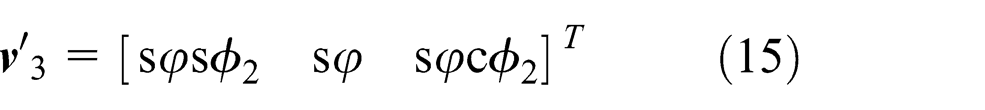
Now, substituting equations (10), (11), and (13)–(15) in the following equation, the vector v _i , with respect to the FCS, is obtained through the serial chain first limb as

$${\mathit{v}}_i={\mathit{R}}_{10}{\mathit{R}}_{11}{\mathit{Tv}\prime }_i$$

(20)

Corresponding to the mechanical structure design of the limb, the manipulator’s geometric parameters are as defined in section “Proposed manipulator”; the angles between the w_i-axis and the v_i-axis are fixed, and the orientation vectors w _i and v _i satisfy the following angle constraint equations

$${\mathit{w}}_i·{\mathit{v}}_i=\cos {\alpha }_2$$

(21)

Equations (2) and (21) are the foundation equations for the solution of kinematics problem in this article. When the pose of the end-effector is known, the joint values can be obtained, thereby the solution of the inverse kinematics issue is completed. Using the expressions derived above, a polynomial solution for the forward kinematics problem will be obtained in the next section.

Forward kinematics solutions

In this article, the approach given here for the derivation of the forward kinematics of the proposed manipulator is based on the solution of the polynomial. As previously mentioned, it is concerned that the structure of this manipulator is decoupled. Therefore, the solution of forward kinematics problem can be divided into two parts: the solutions of the FPKs can be obtained first and then the FOK solutions in this section.

Polynomial solutions for the FPKs

The basic concept of the manipulator has been described by a simple architectural scheme illustrated above. With reference to Figure 4, the position forward kinematics solution is shown at the intersection of point p created by the length of the prismatic actuators l_i. According to equation (2), substitution of points p and q_i gives the following equations

$$(x-x_1{)}^2+(y-y_1{)}^2+(z-z_1{)}^2=(l_{01}+l_1{)}^2$$

(22)

$$(x-x_2{)}^2+(y-y_2{)}^2+(z-z_2{)}^2=(l_{02}+l_2{)}^2$$

(23)

$$(x-x_3{)}^2+(y-y_3{)}^2+(z-z_3{)}^2=(l_{03}+l_3{)}^2$$

(24)

Figure 4.

Position description of the end-effector.

Choosing any two from the above three equations, we can eliminate variable z and obtain two equations with variables x and y. Subtracting equation (22) from equation (23) and equation (22) from equation (24), the following two equations are obtained, which eliminated variable z, and we get the following equations in variables x and y

$$A_{1}x+B_{1}y+C_1=0$$

(25)

$$A_{2}x+B_{2}y+C_2=0$$

(26)

where

$$A_1=2(x_1-x_2)$$

$$B_1=2(y_1-y_2)$$

$$\begin{array}{c}\multicolumn{1}{c}{C_1=x_2^2+y_2^2+z_2^2-x_1^2-y_1^2-z_1^2}\\ +(l_0+l_1{)}^2-(l_0+l_2{)}^2\hfill \end{array}$$

$$A_2=2(x_1-x_3)$$

$$B_2=2(y_1-y_3)$$

$$\begin{array}{c}\multicolumn{1}{c}{C_2=x_3^2+y_3^2+z_3^2-x_1^2-y_1^2-z_1^2}\\ +(l_0+l_1{)}^2-(l_0+l_3{)}^2\hfill \end{array}$$

In order to get the solution of the above equations, we need to eliminate variable y from equations (25) and (26), simultaneously; as a result, the resulting equation will contain only variable x. This equation is

$$\left|\begin{array}{cc}{B}_1\hfill & A_{1}x+C_1\hfill \\ \multicolumn{1}{c}{B_2}& A_{2}x+C_2\hfill \end{array}\right|=0$$

(27)

after expending and simplification, we can get

$$(A_2{B}_1-A_1{B}_2)x+B_1{C}_2-B_2{C}_1=0$$

(28)

In equation (28), coefficients A_i, B_i, and C_i, i = 1, 2, are dependent on the geometric parameters and the lengths of the prismatic actuators l₁, l₂, and l₃; then combining equations (22) and (25), we can get the solution of the forward position of the end-effector.

Polynomial solutions for the FOKs

For the FOK solutions, the key here is to get the expressions of vectors v _i in terms of input angles θ_i3 in the frame FCS (Table 1). And for the purposes of simplifying the equations, the Euler angles, noted as α, β, and γ, are selected according to the orientation of the end-effector in the above section. Since the expressions of v_i have been obtained from equation (20), and the vectors w _i are known, with reference to Figure 5, the kinematic constraint equations describing the forward FOKs satisfy the following relations

$${\mathit{w}}_i·{\mathit{v}}_i=\cos {\alpha }_2,i=1,2,3$$

(29)

Table 1.

Computational results of the FOK problem for the end-effector.

Case	Critical values				Moving platform of orientational vectors
	T	α (rad)	β (rad)	γ (rad)	V 1	V 2	V 3
1	6.1521	2.8193	1.5708	−1.8253	−0.7403, −0.3480, −0.5752	−0.7744, 0.6008, 0.1984	−0.0320, 0.6309, −0.7752
2	−0.4233	−0.8010	1.5708	−2.7175	0.9505, 0.2677, 0.1579	0.4797, −0.2785, −0.8320	0.1109, 0.8469, −0.5201
3	−1.9005	−2.1729	1.5708	1.5372	0.4078, −0.1821, −0.8947	0.7503, −0.6328, 0.1914	−0.3572, −0.8972, −0.2596
4	−1.0429	−1.6128	1.5708	−1.8322	0.8169, 0.0103, −0.5766	−0.3153, 0.3706, −0.8736	0.3009, 0.9536, 0.0097
5	−0.0843	−0.1682	1.5708	0.2571	0.6337, 0.3576, 0.6859	−0.5905, 0.3844, 0.7096	−0.0011, −0.6890, 0.7248
6	1.2986	1.8291	1.5708	−0.4213	−0.9387, −0.1161, 0.3247	−0.5536, 0.5327, −0.6401	−0.3951, −0.6814, −0.6160
7	0.7101	1.2349	1.5708	2.7987	−0.6269, 0.0942, 0.7734	0.4593, −0.4713, 0.7529	0.3931, 0.7351, 0.5524
8	−17.4254	−3.0269	1.5708	1.1416	−0.4012, −0.3532, −0.8452	0.7320, −0.5374, −0.4187	−0.2340, −0.9489, 0.2118

Figure 5.

Orientation kinematic description of the ith limb of the end-effector.

Substituting equations (12) and (20) into equation (29) will lead to three nonlinear algebraic equations in α, β, and γ. Corresponding to the mechanical structure design of the manipulator, angle β can be calculated forwardly from the following equation

$$\cos \beta -\cos {\alpha }_2=0$$

(30)

Therefore, equation (29) can be simplified as two equations and can be written as

$$D_1\sin (\gamma )+E_1\cos (\gamma )+F_1=0$$

(31)

$$D_2\sin (\gamma )+E_2\cos (\gamma )+F_2=0$$

(32)

where

$$\begin{array}{cc}\multicolumn{1}{c}{D_1}& =k_1\sin (\alpha )+k_2\cos (\alpha )+k_3\hfill \\ \multicolumn{1}{c}{E_1}& =g_1\sin (\alpha )+g_2\cos (\alpha )+g_3\hfill \\ \multicolumn{1}{c}{F_1}& =h_1\sin (\alpha )+h_2\cos (\alpha )+h_3\hfill \\ \multicolumn{1}{c}{D_2}& =r_1\sin (\alpha )+r_2\cos (\alpha )+r_3\hfill \\ \multicolumn{1}{c}{E_2}& =s_1\sin (\alpha )+s_2\cos (\alpha )+s_3\hfill \\ \multicolumn{1}{c}{F_2}& =t_1\sin (\alpha )+t_2\cos (\alpha )+t_3\hfill \end{array}$$

In the above equations, the coefficients D_i, E_i, and F_i, i = 1, 2, are functions of the design parameters of the manipulator and of the actuator angles. Detailed expressions of these coefficients are rather cumbersome and are not given here because of space limitation.

From equations (31) and (32), we can find

$$\sin (\gamma )=\frac{E_1{F}_2-E_2{F}_1}{D_1{E}_2-D_2{E}_1}$$

(33)

$$\cos (\gamma )=\frac{D_1{F}_2-D_2{F}_1}{D_2{E}_1-D_1{E}_2}$$

(34)

And then, we substitute the above expressions into the following trigonometric identity

$${\sin }^2(\gamma )+{\cos }^2(\gamma )=1$$

(35)

which leads to an expression containing only one unknown angle α. This expression is written as

$$\begin{array}{c}-D_1^2{E}_2^2+D_1^2{F}_2^2+2D_1{D}_2{E}_1{E}_2-2D_1{D}_2{F}_1{F}_2\hfill \\ -D_2^2{E}_1^2+D_2^2{F}_1^2+E_1^2{F}_2^2-2E_1{E}_2{F}_1{F}_2+E_2^2{F}_1^2=0\hfill \end{array}$$

(36)

In equation (36), substituting the following equivalent expressions for the cosine and sine of the angle α

$$\cos \alpha =\frac{1-t^2}{1+t^2}$$

(37)

$$\sin \alpha =\frac{2t}{1+t^2}$$

(38)

where

$$t=\tan \frac{\alpha }{2}$$

As a result, an eighth-degree polynomial equation in a single variable t is obtained as

$$\sum _{i=0}^n{N}_i{t}^i=0$$

(39)

where N_i, i = 0, 1,…, 8, are the coefficients in terms of the design parameters of the manipulator and the actuator angles.

Consequently, we obtain a first-degree polynomial equation in a single variable x for the FPKs and an eighth-degree polynomial equation in a single variable t for the FOKs. This means that the manipulator may have up to 1 × 8 configurations for a given set of input values.

Simulation and experiment

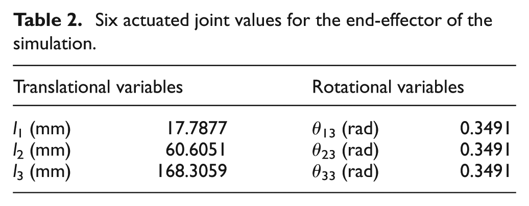
In this section, a numerical simulation for this parallel manipulator is presented to illustrate the above results. The input values of actuated joint are given in Table 2. The solutions of the FPKs are shown in Table 3 and the results of FOKs are shown in Table 1.

Table 2.

Six actuated joint values for the end-effector of the simulation.

Translational variables		Rotational variables
l1 (mm)	17.7877	θ13 (rad)	0.3491
l2 (mm)	60.6051	θ23 (rad)	0.3491
l3 (mm)	168.3059	θ33 (rad)	0.3491

Table 3.

Computation results of the FPK problem for the end-effector.

Positional variables	Case
	β1 > 0	β1 < 0
x (mm)	100	100
y (mm)	100	100
z (mm)	100	−1280

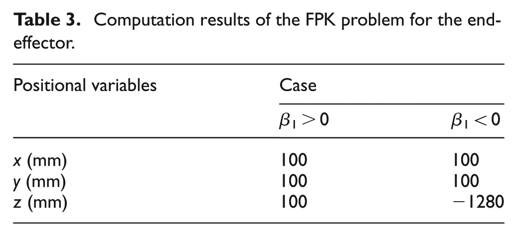
As we can see, there are two real solutions for the FPKs; the configurations are illustrated in Figure 6. However, the according to the initial assemble parameter β₁ of the manipulator, two solutions are not available at the same time for a well mechanical configuration. For this study, as shown in Figure 6(a), the one β₁ > 0 is available. For the FOK solutions, they are all valid. Hence, there are no spurious solutions. As a result, the forward kinematics problem of this manipulator has at most eight real solutions. Based on the solutions, the configurations of the manipulator, including position and orientation of the end-effector, are graphically displayed in Figure 7. A set of experiments are for testing the forward kinematic of the TLPM. Figure 8 shows a sequence of pictures that illustrate the motion capability of the prototype of this manipulator.

Figure 6.

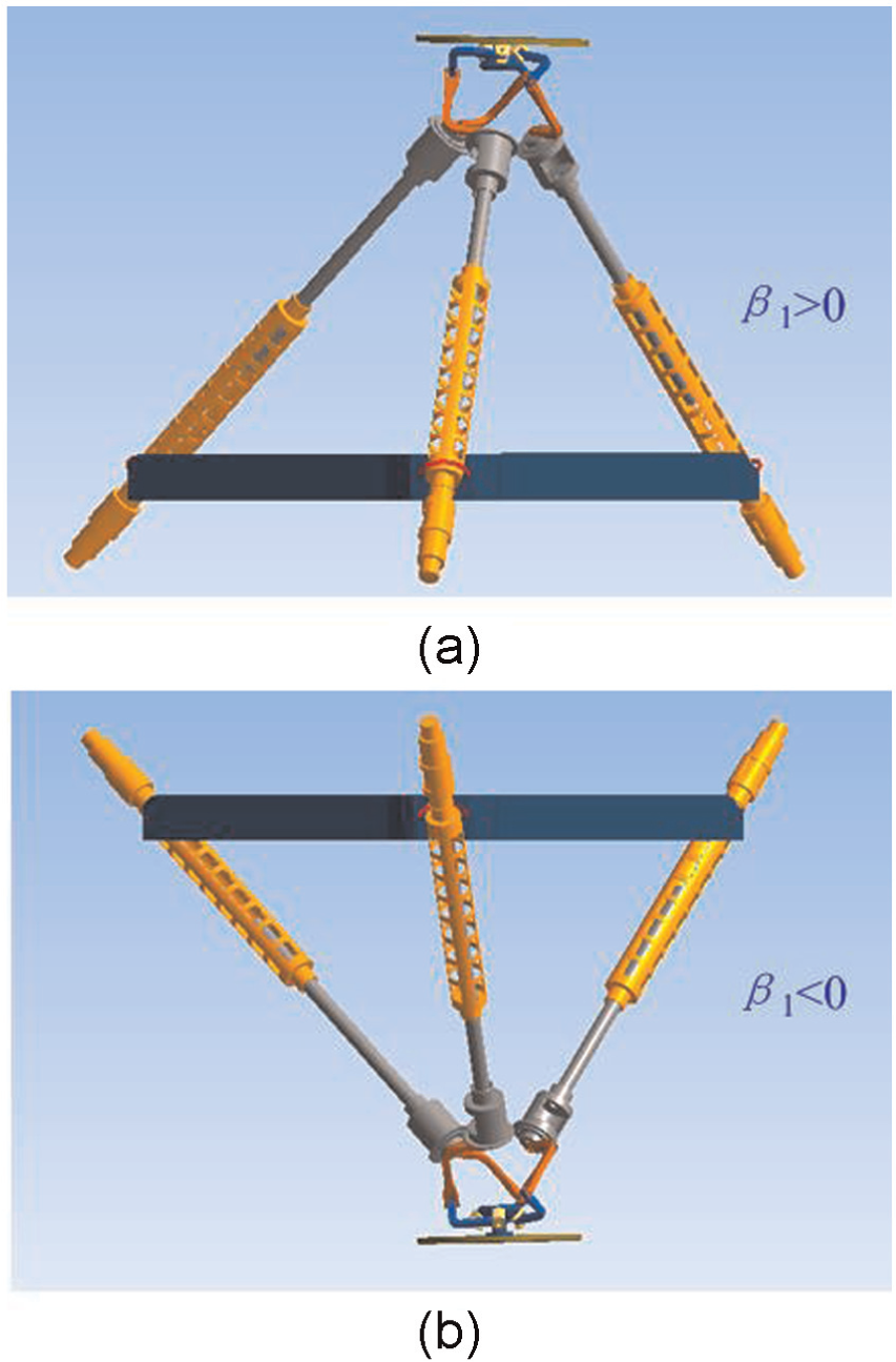
Two solutions of the FPKs for two configurations of the TLPM: (a) β₁ > 0 and (b) β₁ < 0.</ϕχ>

Figure 7.

Eight configurations of the end-effector.

Figure 8.

Motion experiment with forward kinematics of the TLPM.

Conclusion

In this article, the equations for the forward kinematics of a special 6-DOF parallel manipulator have been developed, and the solutions have been shown to be reducible to a first-degree polynomial equation and an eighth-degree polynomial equation. The degree of the equations is relatively smaller comparing to the existing methods, which reduce the computational burden. A numerical simulation is given to verify the algorithm, and the result implies that for a given set of input values, the manipulator can be assembled in at most eight different configurations. And the experiments illustrate the motion ability for forward kinematics of the TLPM. It is also worth noting that the three-limb mechanism is reducible to a low polynomial. Although the results presented in this article are only for the low-degree polynomials. Some of the other methods are well known, but still do not have a uniform method to describe the forward kinematics of the parallel manipulator; therefore, much effort should be devoted.