A model predictive control approach combined unscented Kalman filter vehicle state estimation in intelligent vehicle trajectory tracking

Abstract

Trajectory tracking and state estimation are significant in the motion planning and intelligent vehicle control. This article focuses on the model predictive control approach for the trajectory tracking of the intelligent vehicles and state estimation of the nonlinear vehicle system. The constraints of the system states are considered when applying the model predictive control method to the practical problem, while 4-degree-of-freedom vehicle model and unscented Kalman filter are proposed to estimate the vehicle states. The estimated states of the vehicle are used to provide model predictive control with real-time control and judge vehicle stability. Furthermore, in order to decrease the cost of solving the nonlinear optimization, the linear time-varying model predictive control is used at each time step. The effectiveness of the proposed vehicle state estimation and model predictive control method is tested by driving simulator. The results of simulations and experiments show that great and robust performance is achieved for trajectory tracking and state estimation in different scenarios.

Introduction

Recently, with the development of the intelligent transportation technology, intelligent vehicles have stepped into our daily lives. Google has already tested autonomous cars successfully. Additionally, several automotive companies such as Volvo, Ford, and Tesla have developed new intelligent vehicles with claims that autonomous cars will become available for limited markets by 2030. Another application of autonomous vehicles which has found much interest among researchers is the wheeled robot technology, for various applications such as self-driving in the hazardous environments. ¹ The automated algorithms of vehicle control play a significant role in the self-driving systems. As is well known, the control performance of the intelligent vehicles depends not only on the robust control algorithm but also on the accurate estimation of vehicle state. However, some of the key states are hard to measure directly. Therefore, an online estimation method is necessary to be proposed in the self-driving control.

In the past, Wenzel et al. ² and Baffet et al. ³ proposed to use the dual extended Kalman filter (DEKF) for vehicle state estimation and vehicle parameter estimation, which made use of two Kalman filters (KFs) running in parallel. Best et al. ⁴ considered a real-time state estimation of vehicle handling dynamics by the extended adaptive KF. Chu et al. ⁵ addressed fuzzy logic and KF for the longitudinal vehicle velocity observer. However, for the online and real-time estimation, KF has trouble in handling the nonlinear system estimation; the extended Kalman filter (EKF) needs first-order linearizaion of the nonlinear system, which would lose vehicle nonlinear dynamic characteristics. Ray ⁶ estimated the vehicle dynamic states and the lateral tire forces using the 9-degree-of-freedom (DOF) vehicle model. Imsland et al. ⁷ and Zhao et al. ⁸ explored the nonlinear observers to estimate longitudinal and lateral vehicle velocities. Shraim et al. ⁹ and Ouladsine et al. ¹⁰ estimated velocity and side slip angle by developing a sliding mode observer. However, if the state is unobservable, the state observer would fail.

At the same time, there are numerous dynamics and kinematics constraints of vehicle in the self-driving systems. The model predictive control (MPC) method can handle constraints in a systematic way. It is one of the best ways to process the required system constraints in a wide operating region and close to the boundary of the states and the inputs. Gray et al. ¹¹ presented an active safety system for avoiding obstacles and preventing road departures. The nonlinear model predictive controller (NMPC) was designed with the goal of using the minimum control intervention to keep the driver safe. Gao et al. ¹² and Gray et al. ¹³ proposed a hierarchical control framework used for autonomous and semi-autonomous guidance of ground vehicles; the planned trajectory was tracked by the NMPC method. Abbas ¹⁴ addressed the MPC controller to provide satisfactory online obstacle avoidance and tracking performance by driving simulator with CarSim^®. Moreover, NMPC is difficult to develop in real time, which needs to solve the optimization in each control step. In order to reduce the computational burden, a linearization of the nonlinear plant model in MPC controller was developed to figure out the problem,^{15 –18} and using parallel advances to improve the real-time MPC,^19–21 which can improve the controller computational burden.

In the aforementioned literature, the estimation of the system states is not considered in the control system design process. In this article, the work is presented to investigate the MPC method in the trajectory tracking with the nonlinear state estimation of the vehicle. For state estimation, using the 4-DOF vehicle model combined with the unscented Kalman filter (UKF), the states are estimated to satisfy controllers needed. UKF uses a deterministic sampling approach to capture the mean and covariance estimates with a minimal set of sample points instead of Jacobian matrices. The linear approximators would lose the vehicle and tire nonlinear characteristic in the state estimation. Furthermore, a NMPC tracking problem is transferred to linear time-varying model predictive control (LTV-MPC) in order to do a self-driving tracking control combined with the kinematic model of the vehicle. The proposed method can handle the tracking problem’s state and input constraints and decrease the computational burden in real-time control. The structure of the proposed approach is shown in Figure 1. First, the UKF combined with 4-DOF dynamics vehicle model is developed to estimate the vehicle motion states such as longitudinal velocity, yaw rate, vehicle position, and lateral acceleration, which are passed to the MPC controller in real-time while monitoring vehicle stability. Second, all of the estimation state is provided for system plant to predict the vehicle motion, solve the optimization with vehicle dynamics and kinematics constraints in each control step, and output the control variables to track a given trajectory.

Figure 1.

Structure of the proposed approach.

This article is organized as follows: in section “Vehicle modeling,” the 4-DOF model of the four-wheel vehicle is developed and used for the state estimation, while the vehicle kinematic model is used for trajectory tracking. In section “State estimation and MPC tracking,” the UKF method is used to estimate the state of the vehicle, which is needed for MPC. In addition, LTV-MPC formulation is used to track the reference trajectory and explain how to choose the cost function and build a linearization of a nonlinear plant. Simulations and experimental results are discussed in section “Simulation results.” Conclusions are presented in section “Conclusion.”

Vehicle modeling

Four-DOF vehicle model

Assuming the vehicle is driving on the plane and ignoring the pitch and vertical movement of vehicle, Figure 2 shows a 4-DOF vehicle model which describes the dynamics of the vehicle with four wheels. The DOFs are longitudinal, lateral, yaw, and roll, respectively. The model is utilized for online estimation of dynamic states of the vehicle.

Figure 2.

Vehicle model showing 4 degrees of freedom: longitudinal, lateral, yaw, and roll.

The vehicle dynamics equations are shown as follows

$$\begin{array}{cc}\multicolumn{1}{c}{}& m(\stackrel{·}{u}-\mathrm{rv}-h\phi \stackrel{·}{r}-2\mathrm{hr}\stackrel{·}{\phi })\hfill \\ \multicolumn{1}{c}{}& =F_{\mathrm{xfl}}+F_{\mathrm{xfr}}+F_{\mathrm{xrl}}+F_{\mathrm{xrr}}-F_{\mathrm{yfl}}{\delta }_{\mathrm{fl}}-F_{\mathrm{yf}r}{\delta }_{\mathrm{fr}}\hfill \end{array}$$

(1)

$$\begin{array}{cc}\multicolumn{1}{c}{}& m(\stackrel{·}{v}+\mathrm{ru}+h\stackrel{··}{\phi }-{\mathrm{hr}}^2\phi )\hfill \\ \multicolumn{1}{c}{}& =F_{\mathrm{xfl}}{\delta }_{\mathrm{fl}}+F_{\mathrm{xfr}}{\delta }_{\mathrm{xfr}}+F_{\mathrm{yfl}}+F_{\mathrm{yrl}}+F_{\mathrm{yrr}}+F_{\mathrm{yfr}}\hfill \end{array}$$

(2)

$$\begin{array}{cc}\multicolumn{1}{c}{}& I_z\stackrel{·}{r}-I_{\mathrm{xz}}\stackrel{·}{p}-\mathrm{mh}(u-\mathrm{rv})\phi ={\mathrm{aF}}_{\mathrm{xfl}}{\delta }_{\mathrm{fl}}\hfill \\ \multicolumn{1}{c}{}& +{\mathrm{aF}}_{\mathrm{xfr}}{\delta }_{\mathrm{fr}}+a(F_{\mathrm{yfl}}+F_{\mathrm{yfr}})-b(F_{\mathrm{yrl}}+F_{\mathrm{yrr}})\hfill \\ \multicolumn{1}{c}{}& +\frac{(F_{\mathrm{xfl}}-F_{\mathrm{yfl}}{\delta }_{\mathrm{fl}}-F_{\mathrm{xfr}}+F_{\mathrm{yfr}}{\delta }_{\mathrm{fr}})t_1}{2}\hfill \\ \multicolumn{1}{c}{}& +\frac{(F_{\mathrm{xrl}}-F_{\mathrm{xrr}})t_2}{2}+M_{z1}+M_{z2}+M_{z3}+M_{z4}\hfill \end{array}$$

(3)

$$\begin{array}{cc}\multicolumn{1}{c}{}& (I_x-{\mathrm{mh}}^2)\stackrel{··}{\phi }+m_{s}h(\stackrel{·}{v}+\mathrm{ru})-I_{\mathrm{xz}}\stackrel{·}{r}\hfill \\ \multicolumn{1}{c}{}& -(m_s{h}^2+I_y-I_z)r^2\phi +(k_{\phi 1}+k_{\phi 2})\stackrel{·}{\phi }\hfill \\ \multicolumn{1}{c}{}& +(c_{\phi 1}+c_{\phi 2}-m_s\mathrm{gh})\phi =0\hfill \end{array}$$

(4)

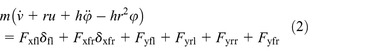
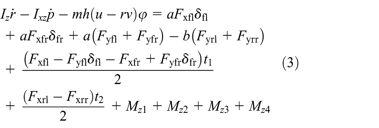
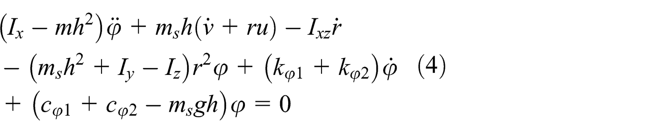
where a is the distance from the front axle to CG, b is the distance from the rear axle to CG, r is the yaw rate, $k_{\mathrm{\phi }i}$ is the damping coefficient at the front and rear axles, h is the height of the roll center, $c_{\mathrm{\phi }i}$ is the roll stiffness, m is the vehicle mass, and $m_s$ is the vehicle sprung mass. The slip angle can be determined by kinematic relationships given as

$${\alpha }_{\mathrm{fl}}={\delta }_{\mathrm{fl}}-\arctan \left(\frac{v+\mathrm{ra}}{u+r\frac{t_1}{2}}\right)$$

(5)

$${\alpha }_{\mathrm{fr}}={\delta }_{\mathrm{fr}}-\arctan \left(\frac{v+\mathrm{ra}}{u-r\frac{t_1}{2}}\right)$$

(6)

$${\alpha }_{\mathrm{rl}}=\arctan \left(\frac{v-\mathrm{rb}}{u+r\frac{t_2}{2}}\right)$$

(7)

$${\alpha }_{\mathrm{rr}}=\arctan \left(\frac{v-\mathrm{rb}}{u-r\frac{t_2}{2}}\right)$$

(8)

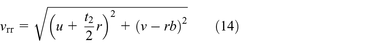
The longitudinal and lateral velocities of the vehicles $u\mathrm{and}v$ , respectively, wheel speed ω and yaw rate r are used to calculate tire slip ratio, as shown in equations (9)–(14).

When the peripheral wheel speed is smaller than the wheel center speed

$$s_{\mathrm{ij}}=1-\frac{{\omega }_{\mathrm{ij}}R}{v_{\mathrm{ij}}},i=f,r;j=l,r$$

(9)

When the peripheral wheel speed is larger than the wheel center speed

$$s_{\mathrm{ij}}=1-\frac{v_{\mathrm{ij}}}{{\omega }_{\mathrm{ij}}R},i=f,r;j=l,r$$

(10)

where $v_{\mathrm{ij}}$ are shown as follows

$$v_{\mathrm{fl}}=\sqrt{{(u+\frac{t_1}{2}r)}^2+{(v+\mathrm{ra})}^2}$$

(11)

$$v_{\mathrm{fr}}=\sqrt{{(u-\frac{t_1}{2}r)}^2+{(v+\mathrm{ra})}^2}$$

(12)

$$v_{\mathrm{rl}}=\sqrt{{(u-\frac{t_2}{2}r)}^2+{(v-\mathrm{rb})}^2}$$

(13)

$$v_{\mathrm{rr}}=\sqrt{{(u+\frac{t_2}{2}r)}^2+{(v-\mathrm{rb})}^2}$$

(14)

The wheel load transfer $F_{\mathrm{zij}}$ on each of four wheels are computed as

$$F_{\mathrm{zij}}=F_{\mathrm{zsij}}\pm \frac{h_g{\mathrm{ma}}_x}{2L}\mp \frac{h_g{\mathrm{ma}}_y}{2t_1},i=f,r;j=l,r$$

(15)

$$F_{\mathrm{zsfj}}=\frac{\mathrm{bmg}}{2(a+b)},F_{\mathrm{zrj}}=\frac{\mathrm{amg}}{2(a+b)},j=l,r$$

(16)

The signs + and − are chosen for each specific wheels, and $a_x\mathrm{and}{a}_y$ are the estimated longitudinal and lateral accelerations, respectively.

The equations of motion can be presented by the following geometric expression

$$\stackrel{·}{X}=u\cos \left(\psi \right)-u\tan \left(\beta \right)\sin \left(\psi \right)$$

(17)

$$\stackrel{·}{Y}=u\sin \left(\psi \right)+u\tan \left(\beta \right)\cos \left(\psi \right)$$

(18)

$$\beta =\arctan \left(\frac{u}{v}\right)$$

(19)

where β is the body slip angle; ψ is the yaw angle; and X and Y are the global x coordinates and global y coordinates, respectively.

Vehicle kinematic model

The kinematic model can be described as

$$\lceil \begin{array}{c}\hfill \stackrel{·}{x}\hfill \\ \multicolumn{1}{c}{\stackrel{·}{y}}\\ \multicolumn{1}{c}{\stackrel{·}{\theta }}\end{array}\rceil =u\lceil \begin{array}{c}\hfill \cos \theta \hfill \\ \multicolumn{1}{c}{\sin \theta }\\ \multicolumn{1}{c}{\tan \frac{\delta }{l}}\end{array}\rceil$$

(20)

The compact form as

$$\stackrel{·}{\mathit{x}}=f(\mathit{x},\mathit{i})$$

(21)

where $(x,y)$ is the position of the vehicle rear axle, θ is the yaw angle of vehicle, l is the wheelbase, and $i(u,\theta )$ is the control input. Figure 3 shows the coordinate system for the vehicle kinematic model.

Figure 3.

Coordinate system of the vehicle kinematic model.

The reference trajectory is defined as follows

$${\stackrel{·}{\mathit{x}}}_{\mathrm{r}}=f(x_{\mathrm{r}},u_{\mathrm{r}})$$

(22)

where $x_{\mathrm{r}}$ is the reference state and $u_{\mathrm{r}}$ is the reference input. The tracking objective is to find a control method to satisfy

$$\begin{array}{cc}\multicolumn{1}{c}{}& \stackrel{·}{\stackrel{~}{\mathit{x}}}=\stackrel{·}{\mathit{x}}-{\stackrel{·}{\mathit{x}}}_{\mathrm{r}}=\left[\begin{array}{ccc}\hfill 0\hfill & \hfill 0\hfill & \hfill -v_{\mathrm{r}}\sin {\theta }_{\mathrm{r}}\hfill \\ \multicolumn{1}{c}{0}& \hfill 0\hfill & \hfill v_{\mathrm{r}}\cos {\theta }_{\mathrm{r}}\hfill \\ \multicolumn{1}{c}{0}& \hfill 0\hfill & \hfill 0\hfill \end{array}\right]\hfill \\ \multicolumn{1}{c}{}& \tilde{\mathit{x}}+\left[\begin{array}{c}\hfill \cos {\theta }_{\mathrm{r}}\hfill \\ \multicolumn{1}{c}{\sin {\theta }_{\mathrm{r}}}\\ \multicolumn{1}{c}{\frac{\tan {\theta }_{\mathrm{r}}}{l}}\end{array}\begin{array}{c}\hfill 0\hfill \\ \multicolumn{1}{c}{0}\\ \multicolumn{1}{c}{\frac{v_{\mathrm{r}}}{l{\cos }^2{\delta }_{\mathrm{r}}}}\end{array}\right]\tilde{u}=A\tilde{x}+B\tilde{u}\hfill \end{array}$$

(23)

As presented in section “Trajectory tracking,” the model prediction control is used in the discrete-time model. Thus, the continuous system needs to transfer to a discrete system. The sampling period is set as T. Euler’s approximation is proposed to obtain the discrete-time model, which is modified by

$$\tilde{x}(k+1)=A_{k,t}\tilde{x}\left(k\right)+B_{k,t}\tilde{u}\left(k\right)$$

(24)

where $A_{k,t}=I+\mathrm{AT}$ , $B_{k,t}=\mathrm{BT}$ , and T is the sample time

$$A_{k,t}=\left[\begin{array}{ccc}\hfill 1\hfill & \hfill 0\hfill & \hfill -v_{\mathrm{r}}\sin {\theta }_{\mathrm{r}}T\hfill \\ \multicolumn{1}{c}{0}& \hfill 1\hfill & \hfill v_{\mathrm{r}}\cos {\theta }_{\mathrm{r}}T\hfill \\ \multicolumn{1}{c}{0}& \hfill 0\hfill & \hfill 1\hfill \end{array}\right],B_{k,t}=\left[\begin{array}{c}\hfill T\cos {\theta }_{\mathrm{r}}\hfill \\ \multicolumn{1}{c}{T\sin {\theta }_{\mathrm{r}}}\\ \multicolumn{1}{c}{\frac{T\tan {\theta }_{\mathrm{r}}}{l}}\end{array}\begin{array}{c}\hfill 0\hfill \\ \multicolumn{1}{c}{0}\\ \multicolumn{1}{c}{\frac{{\mathrm{Tv}}_{\mathrm{r}}}{l{\cos }^2{\delta }_{\mathrm{r}}}}\end{array}\right]$$

(25)

State estimation and MPC tracking

UKF for vehicle state estimation

Julier and colleagues^22,23 proposed to use UKF. Compared with EKF linearizing using Jacobian matrices, the UKF uses a deterministic sampling approach to obtain the mean and covariance estimates with a minimal set of sigma points. The UKF is more powerful than EKF on the nonlinear system in various field applications such as railways, ships, aircrafts, solar probes, and so on.^24–28

Prediction step

We compute a collection of sigma points and form a set of $2\mathrm{n}+1$ sigma points. The columns of ${\chi }_{\mathrm{k}-1}$ are computed by equations (26)–(28)

$${\left({\chi }_{\mathrm{k}-1}\right)}_0={\hat{\mathrm{x}}}_{\mathrm{k}-1}$$

(26)

$${\left({\chi }_{\mathrm{k}-1}\right)}_{\mathrm{i}}={\hat{\mathrm{x}}}_{\mathrm{k}-1}+\sqrt{\mathrm{n}+\mathrm{\lambda }}{\left(\sqrt{{\mathrm{P}}_{\mathrm{k}-1}}\right)}_{\mathrm{i}}$$

(27)

$${\left({\chi }_{\mathrm{k}-1}\right)}_{\mathrm{i}+1}={\hat{\mathrm{x}}}_{\mathrm{k}-1}-\sqrt{\mathrm{n}+\mathrm{\lambda }}{\left(\sqrt{{\mathrm{P}}_{\mathrm{k}-1}}\right)}_{\mathrm{i}},\mathrm{i}=1,\dots ,\mathrm{n}$$

(28)

where $\mathrm{\lambda }={\alpha }^2(\mathrm{n}+\mathrm{k})-\mathrm{n}$ is a scaling parameter, and α and k determine the spread of the sigma points around the mean.

Once ${\chi }_{\mathrm{k}-1}$ is computed, we substitute the sigma points into the dynamic model

$${\left({\hat{\chi }}_{\mathrm{k}}\right)}_{\mathrm{i}}=f\left({\left({\chi }_{\mathrm{k}-1}\right)}_{\mathrm{i}}\right),\mathrm{i}=0,\dots ,2\mathrm{n}$$

(29)

where f is the differential equation defined in equations (1)–(4) for our case. Compute the predicted mean ${\hat{\mathrm{x}}}_{\mathrm{k}}^{-}$ and the predicted covariance ${\mathrm{P}}_{\mathrm{k}}$

$${\hat{\mathrm{x}}}_{\mathrm{k}}^{-}={\displaystyle \sum _{\mathrm{i}=0}^{2\mathrm{n}}}{\mathrm{W}}_{\mathrm{i}}^{\mathrm{m}}{\left({\hat{\chi }}_{\mathrm{k}}\right)}_{\mathrm{i}}$$

(30)

$${\mathrm{P}}_{\mathrm{k}}={\displaystyle \sum _{\mathrm{i}=0}^{2\mathrm{n}}}{\mathrm{W}}_{\mathrm{i}}^{\mathrm{c}}({\left({\hat{\chi }}_{\mathrm{k}}\right)}_{\mathrm{i}}-{\hat{\mathrm{x}}}_{\mathrm{k}}^{-}){({\left({\hat{\chi }}_{\mathrm{k}}\right)}_{\mathrm{i}}-{\hat{\mathrm{x}}}_{\mathrm{k}}^{-})}^{\mathrm{T}}+{\mathrm{Q}}_{\mathrm{k}-1}$$

(31)

where ${\mathrm{Q}}_{\mathrm{k}-1}$ is the process error covariance matrix, and the weights ${\mathrm{W}}_{\mathrm{i}}^{\mathrm{m}}$ and ${\mathrm{W}}_{\mathrm{i}}^{\mathrm{c}}$ are defined as

$${\mathrm{W}}_0^{\mathrm{m}}=\frac{\mathrm{\lambda }}{\mathrm{n}+\mathrm{\lambda }}$$

(32)

$${\mathrm{W}}_0^{\mathrm{c}}=\frac{\mathrm{\lambda }}{\mathrm{n}+\mathrm{\lambda }}+(1-{\alpha }^2+\beta \prime )$$

(33)

$${\mathrm{W}}_{\mathrm{i}}^{\mathrm{m}}=\frac{1}{2(\mathrm{n}+\mathrm{\lambda })},\mathrm{i}=1,\dots ,2\mathrm{n}$$

(34)

$${\mathrm{W}}_{\mathrm{i}}^{\mathrm{c}}=\frac{1}{2(\mathrm{n}+\mathrm{\lambda })},\mathrm{i}=1,\dots ,2\mathrm{n}$$

(35)

$\beta \prime$ is a parameter used to incorporate any prior knowledge about the distribution of $x$ .

Update step

First, compute the sigma points

$${\left({\chi }_{\mathrm{k}-1}\right)}_0={\hat{\mathrm{x}}}_{\mathrm{k}-1}$$

(36)

$${\left({\chi }_{\mathrm{k}-1}\right)}_{\mathrm{i}}={\hat{\mathrm{x}}}_{\mathrm{k}-1}+\sqrt{\mathrm{n}+\mathrm{\lambda }}{\left(\sqrt{{\mathrm{P}}_{\mathrm{k}-1}}\right)}_{\mathrm{i}}$$

(37)

$${\left({\chi }_{\mathrm{k}-1}\right)}_{\mathrm{i}+1}={\hat{\mathrm{x}}}_{\mathrm{k}-1}-\sqrt{\mathrm{n}+\mathrm{\lambda }}{\left(\sqrt{{\mathrm{P}}_{\mathrm{k}-1}}\right)}_{\mathrm{i}},\mathrm{i}=1,\dots ,\mathrm{n}$$

(38)

Then, propagate sigma points through the measurement model

$${\hat{\mathrm{y}}}_{\mathrm{k}}^{\mathrm{i}}=\mathrm{h}\left({\left({\chi }_{\mathrm{k}}^{-}\right)}_{\mathrm{i}}\right),\mathrm{i}=0,\dots ,2\mathrm{n}$$

(39)

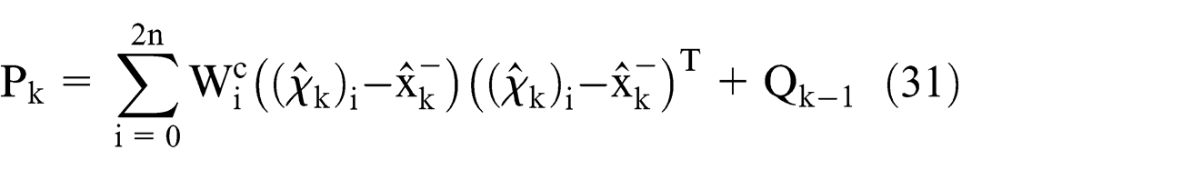
Finally, compute the predicted mean ${\mu }_{\mathrm{k}}$ , the predicted covariance of the measurement ${\mathrm{S}}_{\mathrm{k}}$ , and the cross-covariance of the state and measurement ${\mathrm{C}}_{\mathrm{k}}$

$${\mu }_{\mathrm{k}}={\displaystyle \sum _{\mathrm{i}=0}^{2\mathrm{n}}}{\mathrm{W}}_{\mathrm{i}}^{\mathrm{m}}({\hat{\mathrm{y}}}_{\mathrm{k}}^{\mathrm{i}}-{\mu }_{\mathrm{k}}){({\hat{\mathrm{y}}}_{\mathrm{k}}^{\mathrm{i}}-{\mu }_{\mathrm{k}})}^{\mathrm{T}}+{\mathrm{R}}_{\mathrm{k}}$$

(40)

$${\mathbf{S}}_{\mathrm{k}}={\displaystyle \sum _{\mathrm{i}=0}^{2\mathrm{n}}}{\mathrm{W}}_{\mathrm{i}}^{\mathrm{c}}({\hat{\mathrm{y}}}_{\mathrm{k}}^{\mathrm{i}}-{\mu }_{\mathrm{k}}){({\hat{\mathrm{y}}}_{\mathrm{k}}^{\mathrm{i}}-{\mu }_{\mathrm{k}})}^{\mathrm{T}}+{\mathrm{R}}_{\mathrm{k}}$$

(41)

$${\mathrm{C}}_{\mathrm{k}}={\displaystyle \sum _{\mathrm{i}=0}^{2\mathrm{n}}}{\mathrm{W}}_{\mathrm{i}}^{\mathrm{c}}{(({\chi }_{\mathrm{k}}^{-})}_{\mathrm{i}}-{\mathrm{x}}_{\mathrm{k}}^{-}){({({\chi }_{\mathrm{k}}^{-})}_{\mathrm{i}}-{\mathrm{x}}_{\mathrm{k}}^{-})}^{\mathrm{T}}$$

(42)

where R is the measurement noise covariance matrix. ${\mathbf{K}}_{\mathrm{k}}$ is the filter Kalman gain, and ${\mathbf{x}}_{\mathrm{k}}$ is the filter state mean, and ${\mathbf{P}}_{\mathrm{k}}$ is covariance and ${\mathrm{y}}_{\mathrm{k}}$ is conditional to the measurement.

$${\mathbf{K}}_{\mathbf{k}}={\mathrm{C}}_{\mathrm{k}}{\mathrm{S}}_{\mathrm{k}}^{-1}$$

(43)

$${\mathbf{x}}_{\mathrm{k}}={\mathrm{x}}_{\mathrm{k}}^{-}+{\mathbf{K}}_{\mathbf{k}}({\mathrm{y}}_{\mathrm{k}}-{\mu }_{\mathrm{k}})$$

(44)

$${\mathbf{P}}_{\mathrm{k}}={\mathrm{P}}_{\mathrm{k}}^{-}-{\mathbf{K}}_{\mathbf{k}}{\mathrm{S}}_{\mathrm{k}}{\mathbf{K}}_{\mathbf{k}}^{\mathrm{T}}$$

(45)

Estimation of vehicle states based on UKF

The estimation model of the vehicle dynamics includes the four equations of motion (1)–(4). The state vector ${\mathrm{x}}_{\mathrm{S}}(\mathrm{t})$ consist of longitudinal and lateral velocities (u and v), yaw angle (ψ), yaw rate (r), roll angle, and roll rate (φ and $\stackrel{·}{\phi }$ , respectively), and the tire longitudinal and lateral force vectors $(F_{\mathrm{xfl}},F_{\mathrm{yfl}},F_{\mathrm{xfr}},F_{\mathrm{yfr}},F_{\mathrm{xrl}},F_{\mathrm{yrl}},F_{\mathrm{xrr}},F_{\mathrm{yrr}})$ . Input signal is the front wheel angle δ, while the measurement elements are longitudinal and lateral accelerations ( $a_x$ and $a_y$ ), yaw rate ( $r$ ), and roll rate( $\stackrel{·}{\phi }$ ) with the white noise from CarSim motion sensor. The state vector is shown as follows

$$\begin{array}{cc}\multicolumn{1}{c}{}& {\mathrm{x}}_{\mathrm{S}}\left(\mathrm{t}\right)=\hfill \\ \multicolumn{1}{c}{}& {[uv\psi r\phi \stackrel{·}{\phi }XY{F}_{\mathrm{xfl}},F_{\mathrm{yfl}},F_{\mathrm{xfr}},F_{\mathrm{yfr}},F_{\mathrm{xrl}},F_{\mathrm{yrl}},F_{\mathrm{xrr}},F_{\mathrm{yrr}}]}^T\hfill \end{array}$$

(46)

$$\mathrm{U}\left(\mathrm{t}\right)=\mathrm{\delta }$$

(47)

$$\mathrm{y}\left(\mathrm{t}\right)={[a_x,a_y,r,\phi ]}^T$$

(48)

The nonlinear differential equation is the 16th-order estimation model

$${\stackrel{·}{\hat{x}}}_s\left(t\right)=f(\hat{x},U)+\mathrm{w}$$

(49)

$$\hat{y}\left(t\right)=h(\hat{x},U)+\mathrm{v}$$

(50)

where ${\stackrel{·}{\hat{x}}}_s$ and $\hat{y}(t)$ are the estimation state values, w is the process noise, and v is the measurement noise vector (random zero-mean white noise). $Q(t)=\mathrm{E}({\mathrm{ww}}^{\mathrm{T}})$ is the process-noise covariance matrix and $R(t)=\mathrm{E}({\mathrm{vv}}^{\mathrm{T}})$ is measurement-noise covariance matrix. The UKF method mentioned above is proposed to use the estimate states with equations (1)–(4).

Trajectory tracking

The tracking problem is described in the section “Vehicle modeling.” Trajectory tracking should obtain the vehicle accuracy states in real time. In our case, the longitudinal velocity, yaw angle, and position of the vehicle would be used, which can be estimated by UKF. The control system is presented as above equations (22)–(25). The cost function is used to track the desired trajectory quickly and smoothly. Therefore, the state deviation and control variables are needed for optimization. The cost function in our proposed is given as

$$\begin{array}{cc}\multicolumn{1}{c}{J\left(k\right)=}& {\displaystyle \sum _{i=1}^{M_p}}{\tilde{x}}^T(k+i|t)Q_m\tilde{x}(k+i|t)\hfill \\ \multicolumn{1}{c}{}& +{\tilde{u}}^T(k+i-1|t)R_m\tilde{u}(k+i-1|t)\hfill \end{array}$$

(51)

where $M_p$ is the prediction horizon and $Q_m\mathrm{and}{R}_m$ are the weighting matrices for error state and control variables, respectively. At the same time, the bound of input is given as

$$u_{\min }\le u(k+i|t)\le u_{\max }$$

(52)

The nonlinear optimization problem can be presented as follows

$$min\left\{J\left(k\right)\right\}$$

(53)

subject to

$$\begin{array}{cc}\multicolumn{1}{c}{}& u_{\min }\le u(k+i|t)\le u_{\max }\hfill \\ \multicolumn{1}{c}{}& \stackrel{·}{x}=f(x,u)\hfill \\ \multicolumn{1}{c}{}& x(k|t)=x_0\hfill \end{array}$$

(54)

where $i\in [0,M_p-1]$ and $x_0$ is the initial condition of the state. The nonlinear optimization problem can be solved by the NMPC, but NMPC will take computational effort much higher than linear MPC. It is hard for us to solve the programming function as real time. Moreover, equation (52) cannot limit the increment of the control in each step time, and the mutations cannot be inhibited to affect the continuity of the system. Therefore, the LTV-MPC is proposed in this section to decrease the computational time, and a new cost function is explored as the reference ²⁹

$$\begin{array}{cc}\multicolumn{1}{c}{J\left(k\right)=}& {\displaystyle \sum _{i=1}^{M_p}}\zeta (k+i|t)-{\zeta }_{\mathrm{ref}}{(k+i|t)}_Q^2\hfill \\ \multicolumn{1}{c}{}& +{\displaystyle \sum _{i=1}^{M_c-1}}\Delta U{(k+i|t)}_R^2+\rho {ϵ}^2\hfill \end{array}$$

(55)

where $\zeta (k+i|t)$ is the tracking state of vehicle; ${\zeta }_{\mathrm{ref}}(k+i|t)$ is the reference states for the output tracking variable; $M_p$ is the prediction horizon; $M_c$ is the control horizon; $Q_m,R_m,\mathrm{and}\rho$ are the weighting matrices of appropriate dimensions; and ϵ is a slack variable.

The vehicle position and yaw angle are provided from UKF estimator, which is the kinematic model states as shown in equation (20). The lateral acceleration and yaw rate are used to evaluate the vehicle stability. The time-varying system is explored by the linearization method to transform the optimization problem in every sampling time. Since the function is convex, it is easy to solve the quadratic programming (QP) problems to obtain the optimization solutions. The new state is modified by equation (56), which includes the error of input as one more state

$$\mathrm{\xi }(k|t)=\left[\begin{array}{c}\hfill \tilde{x}(k|t)\hfill \\ \multicolumn{1}{c}{\tilde{u}(k-1|t)}\end{array}\right]$$

(56)

The new state space equation can be described by the following LTV system

$$\mathrm{\xi }(k+1|t)={\tilde{A}}_{k,t}\xi (k|t)+{\tilde{B}}_{k,t}\Delta U(k|t)$$

(57)

$$\zeta (k|t)={\tilde{C}}_{k,t}\xi (k|t)$$

(58)

where

$${\tilde{A}}_{k,t}=\left[\begin{array}{cc}\hfill A_{k,t}\hfill & \hfill B_{k,t}\hfill \\ \multicolumn{1}{c}{0_{m\times n}}& \hfill I_m\hfill \end{array}\right],{\tilde{B}}_{k,t}=\left[\begin{array}{c}\hfill B_{k,t}\hfill \\ \multicolumn{1}{c}{I_m}\end{array}\right]$$

n is the dimension of state, and m is the dimension of control. For the sake of simplicity system, we assume ${\tilde{A}}_{k,t}={\tilde{A}}_{t,t}$ and ${\tilde{B}}_{k,t}={\tilde{B}}_{t,t}$ . The state and system output can be calculated by

$$\xi (t+M_p|t)={\tilde{A}}_{t,t}^{M_p}\xi (t|t)+{\tilde{A}}_{t,t}^{M_p}{\tilde{B}}_t\Delta u(t|t)+\cdots +{\tilde{A}}_{t,t}^{M_p-M_c-1}{\tilde{B}}_t\Delta u(t+M_c|t)$$

$$\zeta (t+N_p|t)={\tilde{C}}_{t,t}{\tilde{A}}_{t,t}^{M_p}\xi (k|t)+{\tilde{C}}_{t,t}{\tilde{A}}_{t,t}^{M_p-1}{\tilde{B}}_t\Delta u(t|t)+\cdots +{\tilde{C}}_{t,t}{\tilde{A}}_{t,t}^{M_p-M_c-1}{\tilde{B}}_t\Delta u(t+M_c|t)$$

In the prediction horizon $M_p$ , and control horizon $M_c$ , the system prediction output equation is given as

$$Y\left(t\right)=\Phi \left(t\right)\xi (t|t)+\mathbf{\Theta }\left(t\right)\Delta U(t|t)$$

(59)

where $Y(t)\mathbf{\Theta }(t)\Delta U(t|t)$ is given as

$$\begin{array}{cc}\multicolumn{1}{c}{}& Y\left(t\right)=\left[\begin{array}{c}\hfill \xi (t+1|t)\hfill \\ \multicolumn{1}{c}{\xi (t+2|t)}\\ \multicolumn{1}{c}{\cdots }\\ \multicolumn{1}{c}{\xi (t+M_c|t)}\\ \multicolumn{1}{c}{\cdots }\\ \multicolumn{1}{c}{\xi (t+M_p|t)}\end{array}\right]\hfill \\ \multicolumn{1}{c}{}& \Phi \left(t\right)=\left[\begin{array}{c}\hfill {\tilde{C}}_{t,t}{\tilde{A}}_{t,t}\hfill \\ \multicolumn{1}{c}{{\tilde{C}}_{t,t}{\tilde{A}}_{t,t}^2}\\ \multicolumn{1}{c}{\cdots }\\ \multicolumn{1}{c}{{\tilde{C}}_{t,t}{\tilde{A}}_{t,t}^{M_c}}\\ \multicolumn{1}{c}{\cdots }\\ \multicolumn{1}{c}{{\tilde{C}}_{t,t}{\tilde{A}}_{t,t}^{M_p}}\end{array}\right]\hfill \\ \multicolumn{1}{c}{}& \mathbf{\Theta }\left(t\right)=\hfill \\ \multicolumn{1}{c}{}& \left[\begin{array}{ccccc}\hfill {\tilde{C}}_{t,t}{\tilde{B}}_{t,t}\hfill & \hfill 0\hfill & \hfill 0\hfill & \hfill 0\hfill & \hfill 0\hfill \\ \multicolumn{1}{c}{{\tilde{C}}_{t,t}{\tilde{A}}_{t,t}{\tilde{B}}_{t,t}}& \hfill {\tilde{C}}_{t,t}{\tilde{B}}_{t,t}\hfill & \hfill 0\hfill & \hfill 0\hfill & \hfill 0\hfill \\ \multicolumn{1}{c}{\cdots }& \hfill \cdots \hfill & \hfill \cdots \hfill & \hfill \cdots \hfill & \hfill \cdots \hfill \\ \multicolumn{1}{c}{{\tilde{C}}_{t,t}{\tilde{A}}_{t,t}^{M_c}{\tilde{B}}_{t,t}}& \hfill {\tilde{C}}_{t,t}{\tilde{A}}_{t,t}^{M_c-1}{\tilde{B}}_{t,t}\hfill & \hfill \cdots \hfill & \hfill \cdots \hfill & \hfill {\tilde{C}}_{t,t}{\tilde{A}}_{t,t}{\tilde{B}}_{t,t}\hfill \\ \multicolumn{1}{c}{\cdots }& \hfill \cdots \hfill & \hfill \cdots \hfill & \hfill \cdots \hfill & \hfill \cdots \hfill \\ \multicolumn{1}{c}{{\tilde{C}}_{t,t}{\tilde{A}}_{t,t}^{M_p-1}{\tilde{B}}_{t,t}}& \hfill {\tilde{C}}_{t,t}{\tilde{A}}_{t,t}^{M_p-2}{\tilde{B}}_{t,t}\hfill & \hfill \cdots \hfill & \hfill \cdots \hfill & \hfill {\tilde{C}}_{t,t}{\tilde{A}}_{t,t}^{M_p-M_c-1}{\tilde{B}}_{t,t}\hfill \end{array}\right]\hfill \\ \multicolumn{1}{c}{}& \Delta U\left(t\right)=\left[\begin{array}{c}\hfill \Delta u(t|t)\hfill \\ \multicolumn{1}{c}{\Delta u(t+1|t)}\\ \multicolumn{1}{c}{\cdots }\\ \multicolumn{1}{c}{\Delta u(t+M_c|t)}\end{array}\right]\hfill \end{array}$$

(60)

The amplitude of constraints in the control incremental input can be rewritten as

$$\begin{array}{cc}\multicolumn{1}{c}{}& u_{min}-u_r(t+k)\le \Delta u(t+k)\le u_{max}-u_r(t+k)\hfill \\ \multicolumn{1}{c}{}& \mathrm{\Delta }{u}_{min}(t+k)\le u(t+k)\le \Delta u_{max}(t+k)\hfill \\ \multicolumn{1}{c}{}& -{26}^{\circ }\le \mathrm{\delta }\le {26}^{\circ }\hfill \\ \multicolumn{1}{c}{}& -0.{47}^{\circ }\le \Delta \mathrm{\delta }\le 0.{47}^{\circ }\hfill \\ \multicolumn{1}{c}{}& \left[\begin{array}{c}\hfill -0.2\hfill \\ \multicolumn{1}{c}{-26}\end{array}\right]\le u_{lim}\le \left[\begin{array}{c}\hfill 0.2\hfill \\ \multicolumn{1}{c}{26}\end{array}\right]\hfill \\ \multicolumn{1}{c}{}& \left[\begin{array}{c}\hfill -0.05\hfill \\ \multicolumn{1}{c}{-0.47}\end{array}\right]\le \Delta u_{lim}\le \left[\begin{array}{c}\hfill 0.05\hfill \\ \multicolumn{1}{c}{0.47}\end{array}\right]\hfill \end{array}$$

(61)

Model predictive controller designed

$$\begin{array}{cc}\multicolumn{1}{c}{J\left(k\right)=}& {\displaystyle \sum _{i=1}^{M_p}}\parallel \zeta (k+i|t)-{\zeta }_{\mathrm{ref}}(k+i|t){\parallel }_Q^2\hfill \\ \multicolumn{1}{c}{}& +{\displaystyle \sum _{i=1}^{M_c-1}}\Delta U{(k+i|t)}_R^2+\rho {ϵ}^2\hfill \end{array}$$

(62)

Now, it is possible to recast the optimization problem in a usual quadratic problem from

$$J\left(k\right)=\frac{1}{2}\Delta U{\left(t\right)}^T{H}_t\Delta U\left(t\right)+G_t^T\Delta U\left(t\right)$$

(63)

where $H_t=2(\mathbf{\Theta }(t{)}^T{Q}_m\mathbf{\Theta }(t)+R_m)$ , $G_t=2\mathbf{\Theta }(t{)}^T{Q}_m\Phi (t)e(t)$ , $e(t)$ is the error of the tracking, $Q_m=\mathrm{diag}(Q,Q,\dots Q)$ , and $R_m=\mathrm{diag}(R,R,\dots ,R)$ .

Simulation results

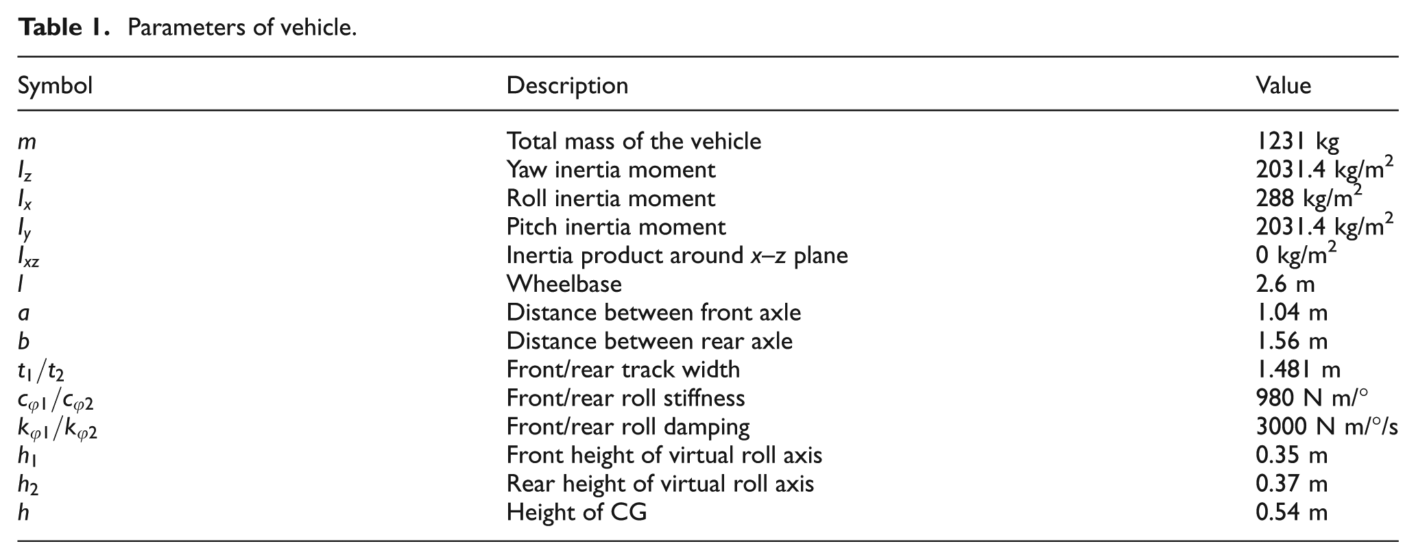
In this section, there are two scenarios to validate the behavior of the proposed state estimation and path-tracking. The first scenario is motion along the straight line tracking in different target longitudinal velocities. The states of the vehicle are also estimated in the driving task. Next, we consider the reference trajectory as an ellipse to validate the lateral tracking capability. In order to evaluate the MPC tracking ability of algorithms and accuracy of estimation, the different velocities and environments are proposed in the simulation. Driving simulator shown in Figure 4 with CarSim is used in all the simulations as reference and set motion sensor as measurement elements in the CarSim. The speed controller used the CarSim driver model. The parameters of the vehicle are shown in Table 1.

Figure 4.

Driving simulator.

Table 1.

Parameters of vehicle.

Symbol	Description	Value
m	Total mass of the vehicle	1231 kg
$I_z$	Yaw inertia moment	2031.4 kg/m2
$I_x$	Roll inertia moment	288 kg/m2
$I_y$	Pitch inertia moment	2031.4 kg/m2
$I_{\mathrm{xz}}$	Inertia product around x–z plane	0 kg/m2
l	Wheelbase	2.6 m
a	Distance between front axle	1.04 m
b	Distance between rear axle	1.56 m
$t_1/t_2$	Front/rear track width	1.481 m
$c_{\mathrm{\phi }1}/c_{\mathrm{\phi }2}$	Front/rear roll stiffness	980 N m/°
$k_{\mathrm{\phi }1}/k_{\mathrm{\phi }2}$	Front/rear roll damping	3000 N m/°/s
$h_1$	Front height of virtual roll axis	0.35 m
$h_2$	Rear height of virtual roll axis	0.37 m
h	Height of CG	0.54 m

Straight line tracking scenario

Figure 5(a) shows the straight line tracking scenario. The original position of the vehicle is (0, 0), and the reference path original point is (5, 5) as shown in Figure 5(a). The function of the reference path is given as

$$\{\begin{array}{c}\hfill y\left(t\right)=x\left(t\right)=\mathrm{ut}\hfill \\ \multicolumn{1}{c}{\phi \left(t\right)=\frac{\pi }{4}}\end{array}$$

(64)

Figure 5.

(a) Different velocity line tracking and (b) different velocity tracking deviation.

where u is the desired longitudinal velocity, and the constraint of the system is the same as (61). Sample time is $T=0.05\mathrm{s}$ , prediction horizon $M_p=50$ , and control horizon $M_c=25$ . The initial velocity is set as the target velocity (10, 20, 30, and 40 km/h). The vehicle initial heading angle is set to 0 rad.

Figure 5(b) describes the tracking deviation in different target longitudinal velocities. The larger initial velocity leads to the larger tracking error. A 40 km/h tracking error is larger than 6 m from 0 to 3 s. Figures 6–8 show the estimation of the vehicle state in which accuracies are achieved by UKF method. Figure 6(a) shows the result of different longitudinal speeds of the vehicle. Figure 6(b) shows the MPC controller output desired speeds. Figures 7 and 8 give us the lateral acceleration and yaw rate in different target longitudinal velocities, respectively. All of the yaw rate is in the reasonable range. However, compared with other tracking speeds, the lateral acceleration of 40 km/h tracking is larger than 0.4 g from 0 to around 3 s, the tire would not work in the linear range, and the vehicle would lose stability. So, the error of tracking is large in the 40 km/h velocity. The tracking model is vehicle kinematic model, which would lose dynamic vehicle characters in the high velocity. In addition, all these estimated states of the vehicle would be provided to the MPC controller for tracking and identifying the vehicle stability. The stability of vehicle and comfort of passengers would be lost in the large lateral acceleration. The estimated states of the vehicle not only provide the control state but also can help us analyze the vehicle stability and change the control method in the different cases.

Figure 6.

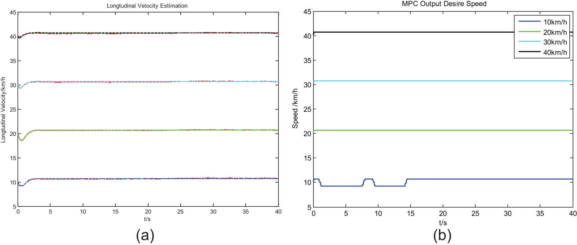
(a) Longitudinal velocity estimation and (b) MPC output desired speed.

Figure 7.

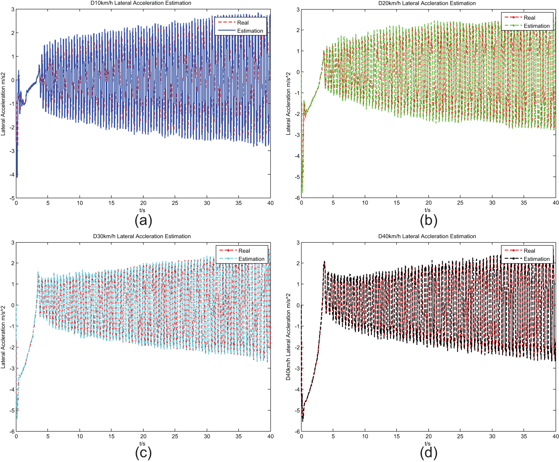
(a) 10 km/h lateral acceleration estimation, (b) 20 km/h lateral acceleration estimation, (c) 30 km/h lateral acceleration estimation, and (d) 40 km/h lateral acceleration estimation.

Figure 8.

(a) 10 km/h yaw rate estimation, (b) 20 km/h yaw rate estimation, (c) 30 km/h yaw rate estimation, and (d) 40 km/h yaw rate estimation.

Ellipse tracking scenario

In this part, the ellipse scenario is proposed to track. The reference path is shown by the parameter equation form

$$\{\begin{array}{cc}\multicolumn{1}{c}{}& x\left(t\right)=24\sin \phi \left(t\right)\hfill \\ \multicolumn{1}{c}{}& y\left(t\right)=40-24\cos \mathrm{\phi }\left(t\right)\hfill \\ \multicolumn{1}{c}{}& \mathrm{\phi }\left(t\right)=0.4\mathrm{ut}\hfill \end{array}$$

(65)

where u is the desired longitudinal velocity. The initial velocity is set to 0. The target velocity is chosen as 10.8, 18, and 36 km/h. The initial time is $t_i=0$ ; the end time is $t_e=40\mathrm{s}$ . The initial state is $x(t_i)=x_0=0$ , $y(t_i)=y_0=0$ . The constraints of the control are obtained the same as equation (61). Sample time is $T=0.05\mathrm{s}$ , prediction horizon $M_p=50$ , and control horizon $M_c=25$ . Figure 9(a) and (b) shows the result of the tracking and the deviation of the tracking, respectively. Figure 9(c) shows the MPC controller output desired speeds. The desired longitudinal velocities 10.8 and 18 km/h can handle the tracking rapidly, and the system deviation tend to zero, while the desired longitudinal velocity 36 km/h is difficult to follow the reference path. The biggest deviation comes from 5 to 10 s and from 20 to 35 s.

Figure 9.

(a) Ellipse tracking, (b) tracking deviation, and (c) MPC desired speeds.

Figure 10(a) shows the longitudinal velocity of vehicle output and estimation. Figure 10(b)–(d) shows the yaw angle real states and estimations, for the 36 km/h yaw angle is too larger to keep safe. Figures 11 and 12 are the lateral acceleration and yaw rate of the vehicle real states and estimations. The results of estimation are really close to the real value. The desired velocity 10.8 and 18 km/h lateral acceleration value is smaller than 0.4 g during the path-tracking as shown in Figure 11(a) and (b). The yaw rate value of 10.8 and 18 km/h is not changed drastically with the path-tracking. In the 36 km/h situation, the lateral acceleration value is changed drastically and is over than 0.7 g from 5 to 10 s. In the 12–17 s and 28–37 s, the accelerations are also larger than 0.4 g (Figure 11(c)). At the same time, the yaw rates are changed a lot (Figure 12(c)). The cases of these situations are hard to track the trajectory for the controller. The stability of the vehicle would be lost during the path-tracking.

Figure 10.

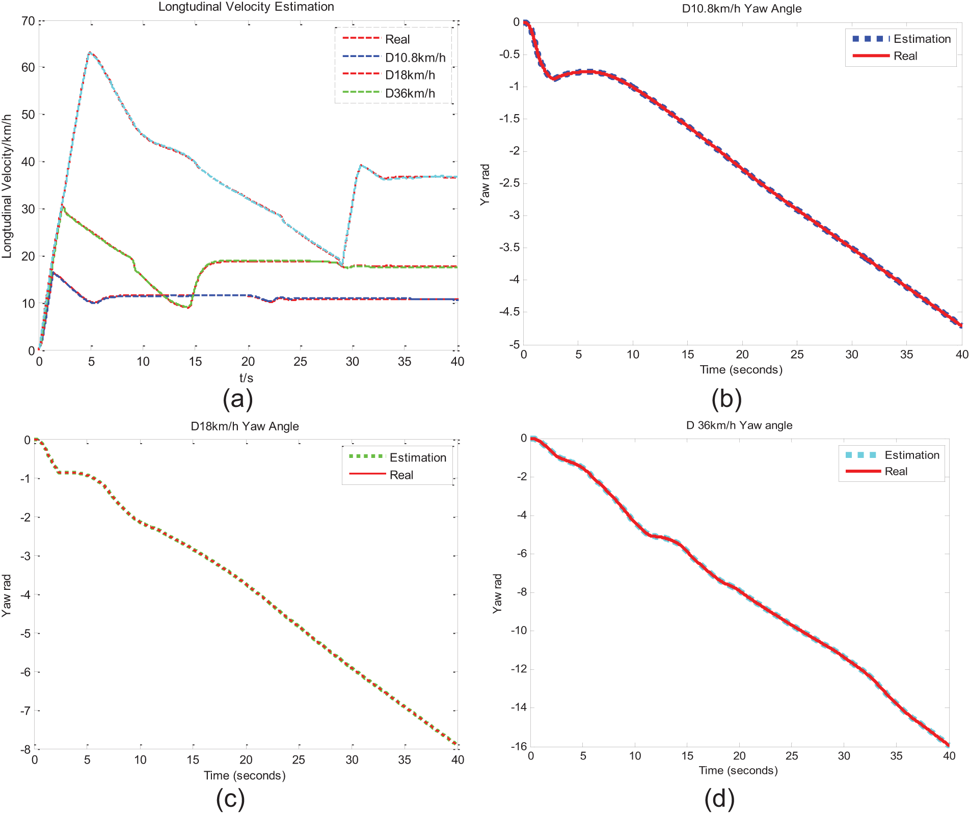
(a) Longitudinal velocity estimation, (b) 10.8 km/h yaw angle, (c) 10.8 km/h yaw angle, and (d) 36 km/h yaw angle.

Figure 11.

(a) 10.8 km/h lateral acceleration, (b) 18 km/h lateral acceleration, and (c) 36 km/h lateral acceleration.

Figure 12.

(a) 10.8 km/h yaw rate estimation, (b) 18 km/h yaw rate estimation, and (c) 36 km/h yaw rate estimation.

Conclusion

In this article, a nonlinear vehicle state estimation using UKF method and trajectory tracking by the MPC approach are proposed, while a LTV-MPC controller is addressed to decrease the computing burden in the real-time control. The capabilities of the method have been simulated in two different scenarios by driving simulator. The first one is the straight line tracking scenario in different target velocities. The other one is the ellipse tracking scenario with different desired velocities. These show good performances for tracking the reference path. The MPC controller shows a high-accuracy solution to track the reference path in the low-velocity case. The state estimation can provide all the vehicle state information for MPC controller such as the position of the vehicle and the yaw angle, which are used for controller, and the lateral acceleration and the yaw rate of the vehicle, which are used to evaluate vehicle stability and keep safe for tracking. In the simulation result, the vehicle lost stability at the large lateral acceleration and yaw rate ratio in the trajectory tracking. The trajectory tracking problem does not only consider the tracking error but also needs to match the stability of the vehicle.

Moreover, the future improvement will aim to propose a method to solve the high-speed tracking control and the nonlinear state estimation with complex tire model. It is not easy to estimate the tire forces and dynamic friction coefficients for the MPC controller, so the controller is limited to accurately tracking in the different surfaces. The mass point model and simple vehicle dynamic model would be applied in the tracking MPC to improve the high-speed tracking and adapt in different surfaces and changed abruptly surfaces.