Disturbance estimation and compensation for planar motors on the long-stroke stage of a wafer stage

Abstract

This article presents a data-based method to estimate and compensate low-frequency disturbance in planar motors on the long-stroke stage of a wafer stage, which is a typical multiple-input multiple-output system. First, a data-based method is introduced to decouple the multiple-input multiple-output system into multi-single-input single-output system, which is crucial for the design of controller and the correction of disturbance estimation in the scanning direction. Second, dominant low-frequency disturbances in the long-stroke stage are analyzed. Third, estimation and compensation method under moving condition is proposed. The compensation method is based on three feedforward tables, and the tables are indexed by trajectory parameters, including velocity and position instead of time in the iterative learning control method. Finally, experiments are performed on the long-stroke stage of a wafer stage to verify the proposed method. Experimental results show that the proposed method can effectively improve the servo performance by reducing the tracking errors by nearly 1/2 in the forward direction and 1/3 in the backward direction and lowering error difference between the forward and backward directions from 5.1 to 1.2 µm.

Introduction

The lithography machines, as shown in Figure 1, require stable and accurate motion for high acceleration and precise synchronization between the wafer stage and the reticle stage. As a multiple-input multiple-output (MIMO) system, the wafer stage tracks motion in both acceleration/deceleration (ACC/DEC) phase and constant velocity phase and thus is an important part of the lithographic machines. However, the wafer stage is susceptible to disturbance forces, including (1) the coupling between multiple degrees of freedom (DOFs) introduced by manufacturing errors, assembly errors, and cable schlepp; (2) the uncertainties caused by redundant actuators; (3) the nonlinear dynamical behaviors of the cable schlepp between the wafer stage and the cable shuttle; and (4) eddy currents in electrically conductive metals. These disturbance forces can be divided based on their frequency. High-frequency disturbances often lead to errors in the ACC/DEC phase, while low-frequency disturbances mainly influence the constant velocity phase.

Figure 1.

Schematic of the lithography machine.

This article focuses on reducing low-frequency disturbance at the constant velocity phase of the wafer stage. To improve servo performance, control systems are included to estimate and compensate disturbance of the wafer stage. To estimate disturbance, a data-based static decoupling method derived from iterative feedback tuning (IFT) algorithm is used to transform the wafer stage from a MIMO system into a multi-SISO system. This method has been used in feedback controller, ¹ feedforward controller,^2–5 and dynamic decoupling. ⁶ To compensate disturbance, different methods have been proposed by previous studies according to sources of disturbance or a single-DOF motion system. In previous works,^3,7–9 a feedforward controller was developed for compensating force ripples. In Hai-Hua et al. ¹⁰ and Bianchi and Bolognani, ¹¹ the cogging force was reduced by an optimal design of controller structure and a lookup table method. In Niu et al., ¹² eddy current reduction was achieved with a finite-element method. In Liu and Peng ¹³ and Shahruz, ¹⁴ observers were developed for disturbance estimation, but this method is too complex to be used in practice. In Butler, ¹⁵ magnetic disturbance has been compensated for a reticle stage with feedforward method. The iterative learning control (ILC)^16–18 is utilized for disturbance compensation in mechanical systems, which is only valid when there is no difference in movement velocity, non-repetitive disturbance, and noise. Moreover, ILC is limited by the position-dependent dynamics of a mechanical motion system.

Nonetheless, as sources of disturbance are rather complex, the above methods cannot ensure stable and accurate motion of the lithography machines. In this article, a disturbance compensation method with multi-lookup tables is proposed. This method compensates low-frequency disturbances according to their features (e.g. position-dependency, direction-dependency or velocity-dependency) instead of sources. A data-based static decoupling method is also presented to ensure that disturbances can be correctly estimated and compensated in the corresponding scanning direction. Comparing with previous methods, the proposed method is applicable to a class of trajectory and no iteration is required.

The remainder of this article is organized as follows. In section “Data-based static decoupling method,” a data-based static decoupling method is presented to decouple the MIMO system into multi-SISO system. Section “Disturbance analysis” discusses the sources of various disturbances in the long-stroke stage. In section “Disturbance estimation and compensation,” the disturbance estimation and compensation approaches are proposed. Section “Experimental results” shows the experimental results and discussion. Finally, this article is concluded in section “Conclusion.”

Data-based static decoupling method

The configuration of planar motors in the long-stroke stage is shown in Figure 2, where the arrows represent the driving force direction of motors; a and b depict the offset from the center of gravity (CoG) of the stage to its center of geometry (CoE) in x and y directions, respectively; F_AX, F_BX, F_CY, and F_DY represent the driving forces produced by the four motors in x and y directions, respectively; L indicates the distance between the force action point of a motor and the CoE. This article aims to improve the servo performance of the wafer stage in the constant velocity phase by compensating the low-frequency disturbance. The scanning direction (x) is concerned. To accurately estimate and compensate the disturbance in x direction, proper static decoupling is required or else the force caused by coupling will cover the true disturbance. The control objective is to minimize the torque force of θ_z around the CoG.

Figure 2.

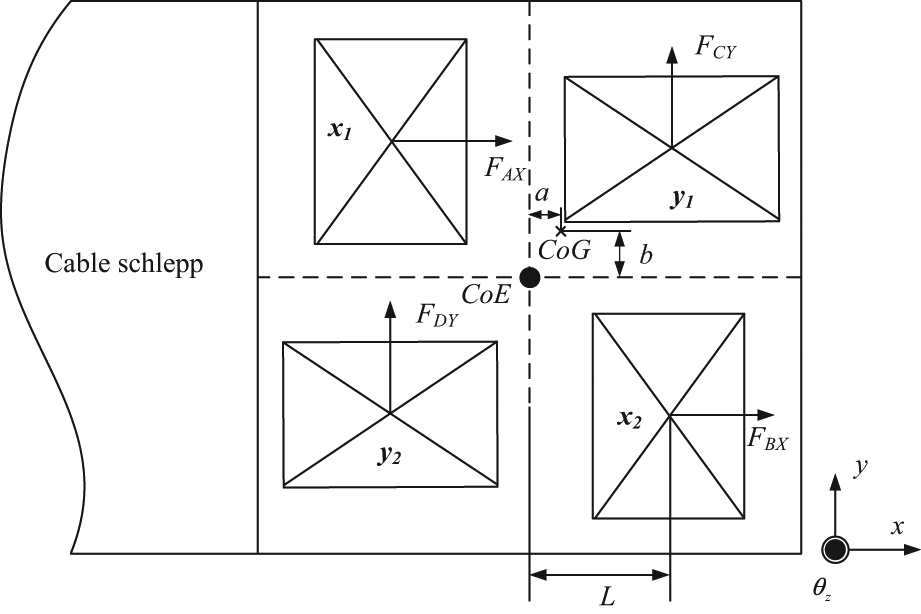
Configuration of planar motors in the long-stroke stage.

Control decoupling

To simplify the decoupling process, two assumptions are made as follows:

1. The motor thrust direction perfectly aligns with the direction shown in Figure 2.

2. All of the four motors have the same distance (L) from their force action points to the CoE.

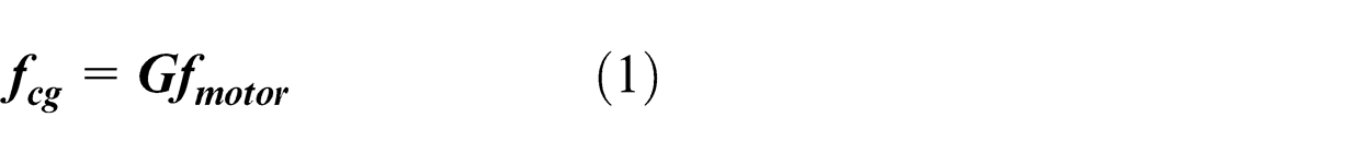
As ${\mathit{f}}_{\mathit{cg}}={[F{\prime }_X,F{\prime }_Y,T{\prime }_Z]}^T$ represents the control force at the CoG, while ${\mathit{f}}_{\mathit{motor}}={[F_{\mathrm{AX}},F_{\mathrm{BX}},F_{\mathrm{CY}},F_{\mathrm{DY}}]}^T$ is the driving force of the four motors, equation (1) can be derived from Figure 2

$${\mathit{f}}_{\mathit{cg}}={\mathit{Gf}}_{\mathit{motor}}$$

(1)

where G is a matrix containing the motor geometry, which can be expressed as

$$\begin{array}{cc}\multicolumn{1}{c}{}& \mathit{G}=\left[\begin{array}{cccc}\hfill 1\hfill & \hfill 1\hfill & \hfill 0\hfill & \hfill 0\hfill \\ \multicolumn{1}{c}{0}& \hfill 0\hfill & \hfill 1\hfill & \hfill 1\hfill \\ \multicolumn{1}{c}{-L(1-{\lambda }_2)}& \hfill L(1+{\lambda }_2)\hfill & \hfill L(1-{\lambda }_1)\hfill & \hfill -L(1+{\lambda }_1)\hfill \end{array}\right]\hfill \\ \multicolumn{1}{c}{}& {\lambda }_1=a/L,{\lambda }_2=b/L\hfill \end{array}$$

(2)

To assign the 3-DOF control effort to the four motors, an additional constraint is required to obtain the inverse of matrix G . With the electrical theory, the energy loss caused by resistance is proportional to the square of current, while the force generated by the motors is proportional to the current. Thus, the optimization objective in equation (3) is selected to minimize the energy loss caused by the motor coil resistance

$$\mathit{J}=min\left(f_{\mathrm{motor}}^T{f}_{\mathrm{motor}}\right)$$

(3)

which is similar to the Moore–Penrose generalized inverse, ¹⁹ thus the following expression is obtained

$${\mathit{f}}_{\mathit{motor}}={\mathit{Df}}_{\mathit{cg}}$$

(4)

where D represents the decoupling matrix, which can be obtained as

$$\mathit{D}={\mathit{G}}^T{\left({\mathit{GG}}^T\right)}^{-1}=\left[\begin{array}{ccc}\hfill \frac{2+{\lambda }_2}{4}\hfill & \hfill -\frac{1}{4}{\lambda }_1\hfill & \hfill -\frac{1}{4L}\hfill \\ \multicolumn{1}{c}{\frac{2-{\lambda }_2}{4}}& \hfill \frac{1}{4}{\lambda }_1\hfill & \hfill \frac{1}{4L}\hfill \\ \multicolumn{1}{c}{-\frac{1}{4}{\lambda }_2}& \hfill \frac{2+{\lambda }_1}{4}\hfill & \hfill \frac{1}{4L}\hfill \\ \multicolumn{1}{c}{\frac{1}{4}{\lambda }_2}& \hfill \frac{2-{\lambda }_1}{4}\hfill & \hfill -\frac{1}{4L}\hfill \end{array}\right]$$

(5)

The control schematic with the decoupling matrix D is illustrated in Figure 3, where ${\mathit{C}}_{\mathit{ff}\prime }(=[C_{\mathrm{ff}}^x,C_{\mathrm{ff}}^y,C_{\mathrm{ff}}^{{\theta }_z}])$ denotes the feedback controller, $\mathit{r}(=[r_x,r_y,r_{{\theta }_z}])$ indicates the desired set point, $\mathit{e}(=[e_x,e_y,e_{{\theta }_z}])$ is the error signal, P represents the controlled plant, and $\mathit{u}(=[u_x,u_y,u_{{\theta }_z}])$ is the control effort.

Figure 3.

Block diagram of control system with the decoupling matrix D .

Data-based parameter identification

In order to realize centralized control (optimal static decoupling), a precise coefficient $\mathit{\lambda }=\left[\begin{array}{cc}\hfill {\lambda }_1\hfill & \hfill {\lambda }_2\hfill \end{array}\right]$ must be obtained. In this article, data-based method is applied and linear time invariant (LTI) system is considered. As ${\mathit{e}}_{{\theta }_z,k}$ represents the affine function of λ at iteration step k, the objective function $\mathit{V}(\mathit{\lambda })$ can be expressed as

$$\mathit{V}(\mathit{\lambda })={\mathit{e}}_{{\theta }_z,k}^{\mathit{T}}(\mathit{\lambda }){\mathit{e}}_{{\theta }_z,k}(\mathit{\lambda })$$

(6)

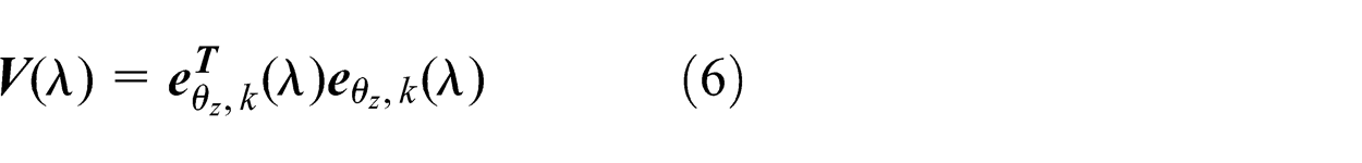
which is a quadratic function of the tracking error in ${\theta }_z$ direction, ${\mathit{e}}_{{\theta }_z,k}(\mathit{\lambda })$ . To minimize the objective function, a second-order Taylor series expansion of $\mathit{V}(\mathit{\lambda })$ about $\mathit{\lambda }$ is considered

$$\begin{array}{c}\multicolumn{1}{c}{\mathit{V}(\mathit{\lambda })\approx \mathit{V}({\mathit{\lambda }}_k)+\nabla \mathit{V}{({\mathit{\lambda }}_k)}^T(\mathit{\lambda }-{\mathit{\lambda }}_k)}\\ \multicolumn{1}{c}{+\frac{1}{2}{(\mathit{\lambda }-{\mathit{\lambda }}_k)}^T{\nabla }^2\mathit{V}({\mathit{\lambda }}_k)(\mathit{\lambda }-{\mathit{\lambda }}_k)}\end{array}$$

(7)

Minimizing equation (7) with the Gauss–Newton update law ²⁰ such that $\mathit{V}({\mathit{\lambda }}_k)\to \mathit{V}({\mathit{\lambda }}_{k+1})$ , then it yields that

$${\mathit{\lambda }}_{k+1}={\mathit{\lambda }}_k-{({\nabla }^2\mathit{V}({\mathit{\lambda }}_k))}^{-1}\nabla \mathit{V}({\mathit{\lambda }}_k)$$

(8)

where $\nabla \mathit{V}$ and ${\nabla }^2\mathit{V}$ indicate the gradient and the Hessian of the objective function, respectively.

To approximate $\nabla \mathit{V}({\mathit{\lambda }}_k)$ and ${\nabla }^2\mathit{V}({\mathit{\lambda }}_k)$ in the data-based method, ²¹ the following expression can be obtained

$$\nabla \mathit{V}({\mathit{\lambda }}_k)=2\nabla {\mathit{e}}_{{\theta }_z,k}^{\mathit{T}}(\mathit{\lambda }){\mathit{e}}_{{\theta }_z,k}(\mathit{\lambda })$$

(9)

$${\nabla }^2\mathit{V}({\mathit{\lambda }}_k)=2\nabla {\mathit{e}}_{{\theta }_z,k}^{\mathit{T}}(\mathit{\lambda })\nabla {\mathit{e}}_{{\theta }_z,k}(\mathit{\lambda })$$

(10)

$${\mathit{\lambda }}_{k+1}={\mathit{\lambda }}_k-{(\nabla {\mathit{e}}_{{\theta }_z,k}^{\mathit{T}}(\mathit{\lambda })\nabla {\mathit{e}}_{{\theta }_z,k}(\mathit{\lambda }))}^{-1}\nabla {\mathit{e}}_{{\theta }_z,k}^{\mathit{T}}(\mathit{\lambda }){\mathit{e}}_{{\theta }_z,k}(\mathit{\lambda })$$

(11)

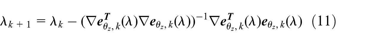
To compute the coefficients λ ₁ and λ ₂, three experiments were implemented. The first experiment was conducted under initial parameter conditions with the wafer stage following an expected trajectory. The initial error signal was ${\mathit{e}}_{{\theta }_z,k}({\lambda }_0)$ with ${\lambda }_1=0$ and ${\lambda }_2=0$ . The second experiment was under a perturbation of λ ₁ with the error signal being ${\mathit{e}}_{{\theta }_z,k}({\lambda }_1+\Delta {\lambda }_1)$ . The third experiment was under a perturbation of λ ₂, thus with the error signal being ${\mathit{e}}_{{\theta }_z,k}({\lambda }_2+\Delta {\lambda }_2)$ .

Then, the first-order Euler approximation of the gradient $\nabla {\mathit{e}}_{{\theta }_z,k}({\lambda }_1)$ and $\nabla {\mathit{e}}_{{\theta }_z,k}({\lambda }_2)$ was calculated by

$$\nabla {\mathit{e}}_{{\theta }_z,k}({\lambda }_1)=\frac{({\mathit{e}}_{{\theta }_z,k}({\lambda }_1+\Delta {\lambda }_1)-{\mathit{e}}_{{\theta }_z,k}({\lambda }_0))}{\Delta {\lambda }_1}$$

(12)

$$\nabla {\mathit{e}}_{{\theta }_z,k}({\lambda }_2)=\frac{({\mathit{e}}_{{\theta }_z,k}({\lambda }_2+\Delta {\lambda }_2)-{\mathit{e}}_{{\theta }_z,k}({\lambda }_0))}{\Delta {\lambda }_2}$$

(13)

Then, the coefficients λ ₁ and λ ₂ were computed according to equations (11)–(13). Therefore, the 3-DOF controllers are rigidly decoupled despite tiny mass variation, which helps to estimate and compensate disturbance.

Disturbance analysis

As shown in Figure 1, the wafer stage can be divided into a long-stroke stage and a short-stroke stage. The long-stroke stage is driven by four linear motors. Each of them has 3 DOFs in the x, y, and θ_z directions. In this way, air bearings and vacuum preloading are restricted for high stiff and non-contact support. To acquire coolant, gas, electrical power, and signals, the long stroke is connected to a cable shuttle with a cable schlepp, as shown in Figure 4. The cable schlepp consists of hoses for transportation of coolant and gas and cables for transportation of electrical power and sensor signals. The cable schlepp is subject to large nonlinear deformation in the x range, which depends on the position of the long-stroke stage in the same direction. The cable shuttle is driven by a linear motor and moves synchronously with the long-stroke stage as a guide only in the y direction between the base-frame and the cable schlepp. Thus, there are various low-frequency disturbances from the cable schlepp and magnetic field in the wafer stage. In this section, sources of low-frequency disturbance in the long-stroke stage are analyzed.

Figure 4.

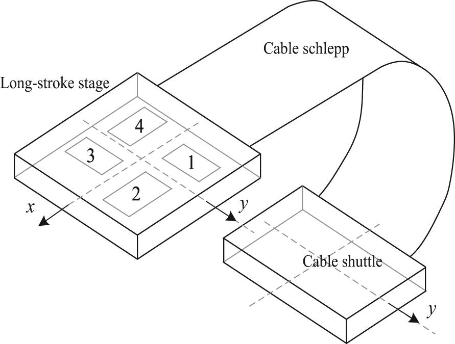
Structure of the long-stroke stage and the cable schlepp.

In the long-stroke stage, there are various sources of disturbance. For example, the irregular magnetic field of the Halbach magnetic array of the permanent planar motors leads to force ripple and cogging force, the eddy current results in velocity-dependent force, and friction causes direction-dependent force. In x direction, the causes of disturbance include the force ripple,^22,23 cable schlepp,^24,25 eddy current, ¹² cogging force,^26,27 friction,^28,29 and reaction force from the short-stroke stage. ³⁰

Among these sources of disturbance, the reaction force is controllable and included in the design of the controller. ²⁷ Thus, the remaining sources of the disturbance include force ripple, cable schlepp, cogging force, and friction. As the force ripple and cogging force are related to the magnetic field, both of them are periodic with the Halbach magnetic array pole pitch. However, the force ripple is related to the current in planar motor coil and the position of the long-stroke stage, but the cogging force is associated with the position of the long-stroke stage.

Besides, magnetic interaction induced by the eddy current is another source of disturbance in the long-stroke stage. According to the principle of electromagnetic induction, when the current in the motor coil varies with time, current is induced in other motor coils and any electrical conductive metals around the coil. As the long-stroke stage is driven by four linear motors that are close to each other, a part of the magnetic field extends outward from the motor itself. Eddy currents in other motors and surrounding conductive metals are induced and are proportional to the stage velocity. As a result, the eddy currents interact with the motor magnetic field, which produces a disturbance force. This force is regarded as a velocity-dependent for the synchronous movement of the motors and surrounding conductive metals.

Moreover, due to the high velocity at the constant velocity phase, Columbia friction is dominant and can be regarded as a direction-dependent force in constant velocity phase. ²⁹ Because of the disturbance caused by cable schlepp, the static restoring force depends on the position and velocity of the long-stroke stage and is the dominant source in constant velocity phase. By contrast, the transient disturbance ²⁵ is dominant in ACC/DEC phase, thus can be neglected in this article.

Disturbance estimation and compensation

In this section, disturbance estimation and compensation methods are investigated. To construct the feedforward tables, the estimated disturbance is represented by the negative of the disturbance force.

Disturbance estimation

Due to the fact that the feedback controller is able to suppress the low-frequency disturbance, the control effort in the x direction can be used to estimate the disturbance when the long-stroke stage is stationary. However, it is not the case for a moving long-stroke stage, thus an improved estimation method is required.

Disturbance estimation under stationary condition

The disturbance estimation process for a stationary long-stroke stage is depicted in Figure 5, where Est is a table for storing the estimated disturbance with the index of the corresponding position and F_d and ${\hat{F}}_d$ represent the actual disturbance and the estimated disturbance, respectively.

Figure 5.

Block diagram of disturbance estimation under stationary condition.

Based on Figure 5 and by assumption that the reference r is zero, the relationship between F_d and ${\hat{F}}_d$ can be expressed as

$$\frac{{\hat{F}}_d}{F_d}=\frac{{\mathrm{PC}}_{\mathrm{ff}}}{1+{\mathrm{PC}}_{\mathrm{ff}}}$$

(14)

The plant P behaves like a double integrator at an extremely low frequency such that the right side of equation (14) is approximate to 1. Thus, it can well estimate the position-dependent disturbance when the long-stroke stage is located at a certain point. Subsequently, the position-dependent disturbance can be accurately estimated with equation (14) when the long-stroke stage is positioned at a series of x position $(x(i)=0.100i(\mathrm{mm}))$ . Then, the control effort $F(x)$ can be estimated and averaged by

$$\begin{array}{cc}\multicolumn{1}{c}{}& \hat{F}\left(i\right)=\frac{1}{N}{\displaystyle \sum _{k=1}^N}{\hat{F}}_i^k\hfill \\ \multicolumn{1}{c}{}& x\left(i\right)=x_0+0.1i\hfill \end{array}$$

(15)

where $N$ is the number of sampling points at each location.

The estimated results of the position-dependent disturbance are shown in Figure 6, where the blue solid line, black dotted line, and red dashed line indicate the disturbance force at x, y, and θ_z directions, respectively.

Figure 6.

Estimated position-dependent disturbance.

From Figure 6, it can be seen that

1. The disturbance at the x direction fluctuates much more than that at the other 2 DOFs, which proves the validity of the decoupling method introduced in section “Data-based static decoupling method.”

2. In the range of [0.05 0.15] m, disturbances at all of the 3 DOFs behave abnormally. The reason is that in this range, part of the wafer stage accessories is located at the edge of Halbach magnetic array.

Disturbance estimation under moving condition

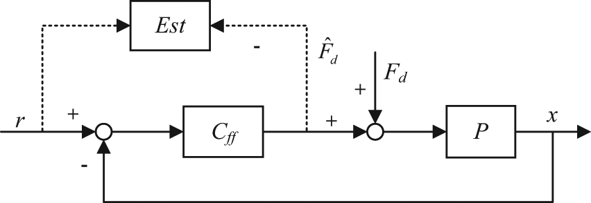
When the stage moves at a high velocity (e.g. 0.25 m/s), the disturbance with the period of pole pitch/8 (i.e. 8.8 mm) reaches a higher degree (e.g. 28 Hz). As aforementioned, method in equation (14) cannot cope with such a kind of disturbance whose frequency reaches a higher degree, thus an improved estimation approach must be developed. Therefore, in this article, an additional transfer function H_f is imposed in series with the lookup table Est to ensure that the transfer function from F_d to ${\hat{F}}_d$ is approximate to 1, as shown in Figure 7.

Figure 7.

Block diagram of improved disturbance estimation method.

Thus, by the assumption that the reference r is zero, the relationship between F_d and ${\hat{F}}_d$ can be expressed as

$$\frac{{\hat{F}}_d}{F_d}=\frac{{\mathrm{PC}}_{\mathrm{ff}}{H}_f}{1+{\mathrm{PC}}_{\mathrm{ff}}}=1$$

(16)

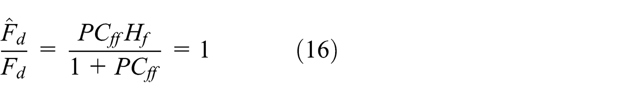
Solving equation (16) gives the value of H_f

$$H_f=\frac{{\mathrm{PC}}_{\mathrm{ff}}+1}{{\mathrm{PC}}_{\mathrm{ff}}}$$

(17)

Then, ${\hat{F}}_d$ can be obtained as

$${\hat{F}}_d=u_{\mathrm{ff}}{H}_f={\mathrm{eC}}_{\mathrm{ff}}{H}_f=\frac{{\mathrm{PC}}_{\mathrm{ff}}+1}{P}e=u_{\mathrm{ff}}+P^{-1}e$$

(18)

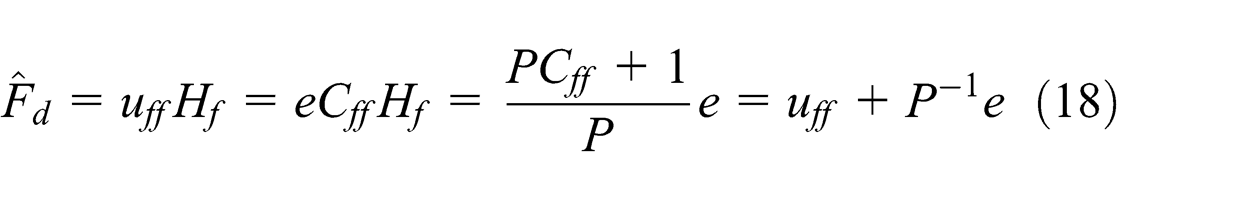
Based on equation (18), Figure 7 can be transformed into Figure 8.

Figure 8.

Block diagram of disturbance estimation under moving condition.

In the constant velocity phase, the flexible modes of the plant are suppressed and P can be approximated by $1/{\mathrm{ms}}^2$ (m representing the mass of the wafer stage). In the discrete domain, the central difference method can be applied. Thus, ${\hat{F}}_d(z)$ can be computed by

$${\hat{F}}_d\left(z\right)=u_{\mathrm{ff}}\left(z\right)+\frac{m(z-2+z^{-1})}{T_s^2}e\left(z\right)$$

(19)

where T_s is the sampling period.

To suppress the disturbance and keep the phase stable, a zero-phase low-pass filter was performed. With a zero-phase filter, data are filtered twice, one in forward direction and the other in backward direction. The estimated disturbance and fitted results with spline fitting method are shown in Figure 9 (only disturbance at 0.04 m/s velocity is shown).

Figure 9.

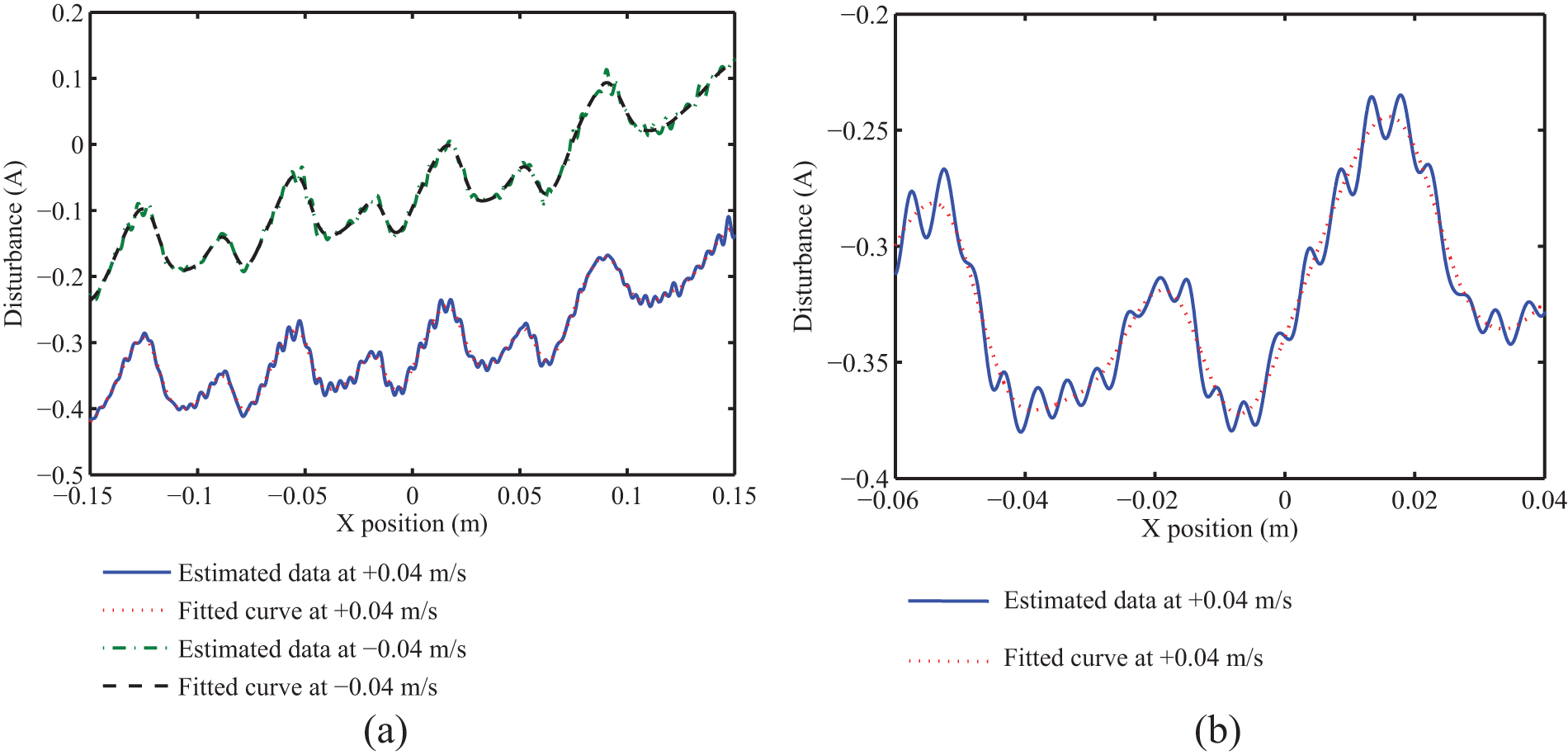
Disturbance at the velocity of 0.04 m/s: (a) disturbance waveforms and (b) zoom figure of (a).

Disturbance compensation

As stated in section “Disturbance analysis,” the low-frequency disturbance can be divided into (a) position-dependent ${\hat{F}}_a$ and (b) velocity-dependent ${\hat{F}}_b$ . The velocity-dependent can be further split into (b1) direction-dependent and (b2) velocity- and direction-dependent.

To design the compensation table, ${\hat{F}}_d$ was first estimated with a series of constant velocity based on the proposed estimation process shown in Figure 8. Then, the estimated data were processed with equations (20)–(22), and the results are shown in Figures 10 and 11. Figure 10 shows the position-dependent and velocity-dependent disturbances obtained by equations (20) and (21), respectively, while Figure 11 shows the mean of velocity-dependent disturbance versus the velocity according to equation (22)

$${\hat{F}}_a=\frac{1}{2}({\hat{F}}_{d,\mathrm{forward}}+{\hat{F}}_{d,\mathrm{backward}})$$

(20)

$${\hat{F}}_b=\frac{1}{2}({\hat{F}}_{d,\mathrm{forward}}-{\hat{F}}_{d,\mathrm{backward}})={\hat{F}}_{b1}+{\hat{F}}_{b2}$$

(21)

$$\mathrm{Offset}\left(v\right)=\mathrm{mean}\left({\hat{F}}_b\left(v\right)\right)-\mathrm{mean}\left({\hat{F}}_b(0.04)\right)$$

(22)

Figure 10.

Disturbance at different velocities: (a) position-dependent disturbance and (b) velocity-dependent disturbance.

Figure 11.

Mean of velocity-dependent disturbance versus velocity.

It can be seen from Figure 10(a) that the position-dependent disturbance slightly varies with the increase in velocity as the velocity is higher than 0.04 m/s. The difference at the two low velocities is caused by the difference in velocity-dependent disturbance in the forward and backward directions. Therefore, position-dependent force at any velocity higher than 0.04 m/s can be represented by that estimated at the velocity of 0.04 m/s.

As shown in Figure 10(b), the velocity-dependent disturbance curves are nearly parallel to each other when the velocity is higher than 0.04 m/s. Figure 11 indicates that the mean of velocity-dependent disturbance nearly follows a linear relationship with the velocity. Due to the two above-mentioned properties, the velocity-dependent disturbance at 0.20 m/s can be represented with the curve of 0.04 m/s and an offset, equaling to the difference between the means of data at 0.20 and 0.40 m/s.

Thus, the disturbance compensation scheme with Tables 1–3 in Figure 12 can be performed, as shown. Table 1 is used to store the position-dependent force at 0.04 m/s and indexed with the reference position r. Table 2 is applied to store the velocity-dependent force at 0.04 m/s and indexed with the reference position r and the direction of motion, which can be obtained by Sgn(v). Table 3 stores the offset and is indexed with velocity v. All the tables are designed with two steps: (1) fitting the estimated data with spline as shown in Figure 9 and (2) resampling the estimated data to gain the table.

Table 1.

MAE in the compensation window.

Type		MAE (µm)
Forward	Without compensation	21.4
	With compensation	12.5
Backward	Without compensation	16.3
	With compensation	11.3

MAE: maximum absolute error.

Figure 12.

The lookup table-based compensation scheme.

Experimental results

To verify the validity of the proposed compensation method, experiments were performed on the long stroke of a wafer stage. As shown in Figure 13, the test bench consists of a motion controller, a data process unit, motor drivers, long-stroke motors, a long-stroke stage, digital-to-analog (D/A) converters, and analog-to-digital (A/D) converters. The position of long-stroke stage was measured by the position sensitive detector (PSD) and optical grating scale. The sampling frequency of digital control system was 5000 Hz. A fourth-order trajectory was adopted. ³¹ The velocity was set as 0.20 m/s, and the scaled acceleration profile is shown in Figure 14 (green dashed line). It is worth mentioning that during the experiments, the three tables were interpolated to extend the data.

Figure 13.

Scheme of hardware connection.

Figure 14.

Tracking error: (a) error in forward direction, (b) zoom figure of (a), (c) error in backward direction and (d) zoom figure of (c).

The results are shown in Figure 14 and Table 1. Figure 14(a) and (b) show the tracking error in forward direction, while Figure 14(c) and (d) show that in backward direction. Furthermore, the compensation window is given in Figure 14 to describe the results more clearly. Table 1 shows the comparison results of the maximum absolute error (MAE).

With all the results, it can be seen that with the proposed compensation method, the maximum tracking error is reduced by nearly 1/2 in forward direction and nearly 1/3 in backward direction. Besides, the estimation error is reduced from 5.1 to 1.2 µm between the forward direction and the backward direction. This indicates that the direction-dependent disturbance at constant velocity phase is reduced and thus is beneficial for the repetitive motion of the wafer stage. Additionally, the tracking error at the beginning of ACC/DEC phase is diverted due to step-increasing, because with the introduction of the compensation table, the acceleration calculated before compensation cannot be applied at the beginning of compensation but needs to be recalculated.

Conclusion

The long-stroke stage in a wafer stage is influenced by disturbances from the cable schlepp, magnetic field and other sources, which reduce the stability and accuracy of motion. To improve the performance of the wafer stage, this article aims to reduce the low-frequency disturbance in the constant velocity phase by providing accurate estimation and compensation for the planar motors on the long-stroke stage. The wafer stage, as a MIMO system, is decoupled into a multi-SISO system with a data-based method, so as to simplify the design of controller and estimate disturbance. By analyzing sources of low-frequency disturbance, a disturbance estimation method under moving condition and a compensation approach with multi-tables are proposed. The proposed estimation method can effectively evaluate the position-dependent disturbance, while the proposed compensation method requires no iteration and can be applied to a class of motion profile since the feedforward tables are indexed by trajectory parameters, including velocity and position instead of time in ILC method. To verify the proposed methods, experiments were conducted on the long-stroke stage of a wafer stage. Experimental results show that tracking errors were reduced by nearly 1/2 in the forward direction and 1/3 in the backward direction, and error difference between the forward and backward directions was lowered from 5.1 to 1.2 µm. Importantly, the proposed approach is not restricted to the long stroke, but can be used in other similar systems. Future work should focus on studying the combination of the proposed method with ILC and whether it can be used in other mechanical systems.