Sage Journals: Discover world-class research

Abstract

This article introduces the basic theory of modal analysis. The modal testing system is established for a developing truck body. Using a pseudo-random excitation signal along the x, y, and z directions, the modal test is carried out to obtain the dynamic performance by multi-point excitations. The transfer function set is obtained by averaging all transfer functions, and the set is processed by order selection to get 28 order modes. Fitting modal parameters and normalizing modal mass can gain natural frequencies and vibration modes of cab. Then, the modal analysis of truck cab is calculated based on the finite element method, and the results are compared with the test results. The improved measures are put forward to enhance the local stiffness, avoid modal coupling, and reduce vibration noise. So, this article supplies a reference for the dynamic test for the large body.

Keywords

Modal test dynamic characteristics truck body transfer function

Introduction

With the rapid growth of buildings, long-range transportation, and logistics, the heavy lorry has a huge development in the automotive industry¹ because of the advantage of dead-weight. In the running process, extrinsic and intrinsic motivations, induced by the uneven surface of road, the change of speed and direction, the vibration coming from wheel, engine and transmission system, the impact of gear, and so on easily cause a strong vibration of cab. The vibration brings many disadvantages, such as making the driver and passengers feel uncomfortable, bringing noise and fatigue failure of components, damaging the protective layer and sealing capacity, and weakening the corrosion resistance of the cab.² Therefore, the modal analysis of cab body-in-white (BIW) is important. Especially, the low-order elastic modal reflects the stiffness performance of the whole vehicle body and is the key parameter to control the vibration of vehicle.^3,4

There are also many studies on the technique of modal parameter identification. Experimental modal analysis (EMA) or modal testing is an important engineering technique to determine the structural modal parameters. And EMA can be combined with the computer-aided engineering (CAE) that provides theoretical simulation to verify the structural theoretical model, and hence, the virtual testing can be implemented to assist product design and development.^5–7 In the late 1960s, Cole and Henry⁸ proposed a random decrement technique (RDT) based on the single-point excitation and single-order modal testing and applied it to the modal parameter identification of space shuttle. The random decrement method is a single-channel signal, which cannot be directly used for modal parameter identification.⁹ Using the response signal in time domain, Ibrahim¹⁰ put this technology into the field of multi-channel signals. With the development of the modal analysis technology, Ibrahim time domain (ITD) identification was put forward. This method can identify the modal parameters only using response without inputs; therefore, it can be only applied to Gaussian distribution whose mean value of response signal is zero. And it needs many tests, so it is easy to be interfered by noise and has high signal-to-noise ratio.¹¹ Box et al.¹² proposed a time-series analysis method used in modal analysis, and this approach did not produce energy leak, had high resolution, and can be used for real-time online modal analysis, but it can only identify local modal and cannot describe the overall modes under white noise excitation.^13,14

Brown et al.¹⁵ put forward a least-squares complex exponent (LSCE) method to identify the modal parameters of multiple responses, which is a single–reference point complex exponential (SRCE) method. Yu¹⁶ adopted the single-input multi-output analysis method to obtain the modal parameters of white body, compared with the finite element simulation results, in order to optimize the design of the body. Because of uneven distribution of energy in the system, the method is applied to the local mode identification. Van der Auweraer et al.¹⁷ and Verboven¹⁸ developed a least-squares complex frequency domain (LSCF) method to identify modal parameters in frequency domain. This method is more widely used, but there are many defects, such as power consumption, truncation error, frequency aliasing, and off-line analysis. In time domain, the modal parameter identification can be carried out only using response signal; therefore, it can make the real-time online modal analysis for cars and other structures to reflect the actual dynamic performance.

Based on SRCE method, Leuridan and Vold¹⁹ and Vold et al.²⁰ presented a poly–reference point complex exponential (PRCE) method, which extracted the natural frequencies according to incentive and response signals. Compared with the SRCE, it expanded the amount of data information, and the energy distribution was more even in the system. The real and complex modes can be identified, and the extracted modal parameters are more complete. In addition, this method has the strong ability to recognize the intensive and multiple root mode, and the identification accuracy is greatly improved. Ma et al.²¹ used PRCE to get modal parameter identification of a car BIW, and the test results agreed with the simulations.

Due to a large number of truck under long-distance freight work, the drivers have to drive in a long time with heavy load, so the high request is put forward for the heavy truck comfort.^22,23 The multi-point excitations are widely adopted in order to get more accurate modal parameters in modal test for vehicle, but the most modal tests are based on the assumption of stationary white noise excitation. In this article, considering the pseudo-random signal as the incentive in order to simulate the actual environment accurately, the dynamics parameters of a heavy truck are solved using the least squares method as parameter identification and adopting multi-point pulsing and multiple points receiving approach. Then, using the finite element method (FEM) to solve kinetic parameters under modal coordinates,^24,25 this article describes the contrast analysis between the simulation results and the test to check the validity of the experiment. So, this article supplies a reference for the dynamic test for the large body.

Theory of modal analysis

The modal test theory is to test the system by the dynamic measuring technology.^26,27 By processing input and output signals, the testing transfer function is identified to get the inherent characteristics using modal parameters. The motion equation can be expressed as

[M] {\overset{\cdot\cdot}{x} (t)} + [C] {\overset{\cdot}{x} (t)} + [K] {x (t)} = {f (t)}

(1)

where [M] is the mass matrix, [C] is the damping matrix, [K] is the stiffness matrix, x is the displacement, f is the exciting force, and t is the time.

Equation (2) was derived from equation (1) based on Laplace transform (s is a variable), considering the initial displacement and velocity as zero

(s^{2} [M] + s [C] + [K]) {X (s)} = {F (s)}

(2)

\begin{matrix} [Z (s)] {X (s)} = {F (s)} \\ [Z (s)] = {X (s)}^{- 1} {F (s)} = (s^{2} [M] + s [C] + [K]) \end{matrix}

(3)

where [Z(s)] is the generalized impedance of system.

The modal analysis by FEM is based on the “Reticulation” material characteristics to get the mass matrix [M] and stiffness matrix [K]. For the linear or weak damping system, their damping matrix [C] is considered as proportional damping: $C = c^{k} K + c^{m} M$ . Then, based on matrix diagonalization and normal modes, equation (4) can be deduced using equation (2)

X (s) = F (s) {(s^{2} M + K)}^{- 1}

(4)

Transfer function matrix $[H (s)]$ is defined as

{X (s)} = [H (s)] {F (s)}

(5)

So, equation (6) is expressed as

[H (s)] = {[Z (s)]}^{- 1} = (s^{2} [M] + s [C] + {[K])}^{- 1}

(6)

Equation (6) is converted to

[H (s)] = {[Z (s)]}^{- 1} = \frac{adj ([Z (s)])}{[Z (s)]}

(7)

EMA is the inverse process of equation (4). To the known input and output signals, the mass matrix, damping matrix, and stiffness matrix can be solved using formula (6).^25,28

Modal test of truck cab

Theory of modal test

Using LSCE method,^17,18 the modal parameters are identified based on equation (3). In modal test, LSCE is a time domain poly-reference method, which can identify the complete modes by residue. Formula (3) can be expanded in terms of residue at pole using inverse Laplace transformation

h (t) = \sum_{r = 1}^{N} (A_{r} e^{P_{r}, t} + A_{r}^{*} e^{p_{r}^{*} t})

(8)

After sampling, $Z_{r} = e^{P_{r} Δ t}$ and $h_{n} = h (n Δ t)$ , according to the relationship of the modal vectors V, modal participation factor matrix L, and the residue, Formula (8) is

h_{n_{k}} = \sum_{r = 1}^{N} (V_{kr} Z_{r}^{n} L_{r} + V_{kr}^{*} Z_{r}^{n^{*}} L_{r}^{*})

(9)

where n is the number of sample points, k is the degree of freedom system, and N is the residue needing to fit (modal number). The regression equation is defined as

L_{r} (Z_{r}^{n} I + Z_{r}^{p - 1} A_{1} + \dots + A_{p}) = 0

(10)

Based on regression equation (10), formula (9) can be deduced to

h_{n} I + h_{n} A_{1} + \dots + h_{n - p} A_{p} = 0

(11)

All sample points can constitute Hankel matrix,²⁹ which can be written in the form of row vector

[\begin{matrix} h_{(1) {(p - 1)}_{1}} \dots h_{(1) {(0)}_{1}} \\ ⋮ ⋮ \\ {h_{(N_{t} - 1) (p - 1)}}_{_{1}} \dots h_{(N_{t} - p) {(0)}_{1}} \\ ⋮ ⋮ \\ h_{(1) {(p - 1)}_{N_{0} N_{i}}} \dots h_{(1) {(0)}_{N_{0} N_{i}}} \\ ⋮ ⋮ \\ h_{(N_{t} - 1) {(p - 1)}_{N_{0} N_{i}}} \dots h_{(N_{t} - p) {(p - 1)}_{N_{0} N_{1}}} \end{matrix}] [\begin{matrix} A_{1} \\ A_{2} \\ \dots \\ A_{p} \end{matrix}] = [\begin{matrix} - h_{p 1} \\ ⋮ \\ - h_{{(N_{t})}_{1}} \\ ⋮ \\ - h_{p N_{0} N_{i}} \\ ⋮ \\ - h_{{(N_{t})}_{N_{0} N_{i}}} \end{matrix}]

(12)

where the first subscript of h is the sample point, from 1 to $N_{t}$ ; the second subscript of h is the modal order, from $p - 1$ to 0; the third is the degree of freedom system, from 1 to $N_{0} N_{i}$ ; $N_{0}$ is the output degree of freedom; and $N_{i}$ is the input degree of freedom.

The overdetermined equation (12) is solved by using the least squares method to obtain all the residues. Then, the system poles can be obtained based on the above residues and equation (10). Modal shape, mass, stiffness, damping ratio, and so on are identified according to the relationship among the modal parameters.

Establishment of the test system

Composition of the test system

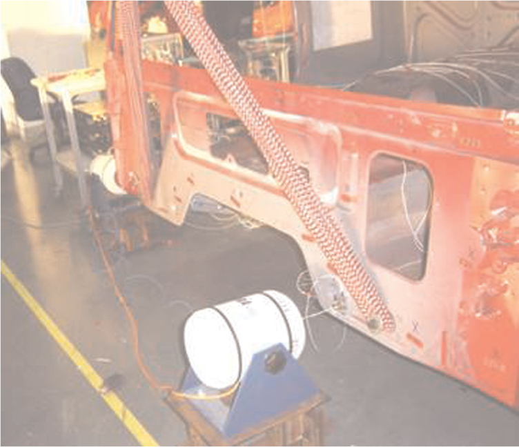
Experimental system consists of three parts: excitation system, response pick-up system, and modal process analysis systems.^30–32 (1) Excitation system: Quad Digital-to-Analog Converter (QDAC) signal generation module, the power amplifier, and exciter of LMS SCADAS III SC316W; (2) response pick-up system: integrated circuit piezoelectric (ICP) acceleration sensor, ICP force sensor, signal amplification of LMS SCADAS III SC316W, and smart data acquisition system; (3) modal process analysis system: LMS Test.Lab.³³ The test system is described in Figure 1.

Figure 1.

The test system.

Experiment scheme

In the modal test, the truck cab was in a free state and suspended with rubber rope. The truck body was hung on the front and rear ends of the left and right longerons using a rubber rope, and it was in four-point suspension status. The cab body was kept balanced as the front hitch point was located in the installation position of bumper, and the rear hitch point was situated in the holes of cab stringer. The lower end of the rubber rope was connected to the cab by a hook, and the upper end was connected to honing car through a pulley.^34,35 The suspension is shown in Figure 2.

Figure 2.

The hitch positions of truck cab in modal test.

The appropriate excitation signal can provide enough energy and excite all the modes in test, so pseudo-random excitation signal was chosen under the frequency range of 0–200 Hz. Multi-point excitations and multi-point responses (x, y, and z three-way responses) can prevent the loss of important information and avoid the incomplete mode.

In experiment, the excitation points were measured by triaxial sensor, and the pick-up points were tested in seven batches. Each batch included 30 moving sensors to test along the three, x, y, and z, directions. The method of collecting signal increased the experiment workload but improved the test accuracy. The front end of longeron was defined as X exciting direction, which was shown in Figure 3. The front end of right threshold beam was considered as Y exciting direction, shown in Figure 4. The rear end of longeron was Z exciting direction, shown in Figure 5.

Figure 3.

The exciting point in X direction.

Figure 4.

The exciting point in Y direction.

Figure 5.

The exciting point in Z direction.

A total of 213 collection points were identified as shown in Figure 6, and their distribution was as follows: 40 points were located in firewall, 64 points in side plates, 43 points in floorboard, 29 points in roof panel, and 37 points in rear quarter panel.

Figure 6.

The layout of test points.

Collection of experiment data

During collection, the transfer and coherence functions of test data were simultaneously processed. The signal was valid when coherent coefficient was above 0.8.^36,37 Collecting signals while processing them can improve the precision and avoid repetitive trials. Coherence in x, y, and z directions was shown in Figures 7 –9, respectively. The coherent coefficient of few frequencies was below 0.8, and the rest was close to 1. Because of the good correlation between measuring points and excitation points, the signal-to-noise ratio was high and excitation was effective.

Figure 7.

Coherence in x direction.

Figure 8.

Coherence in y direction.

Figure 9.

Coherence in z direction.

The response acceleration was tested and analyzed in three, x, y, and z, directions. All transfer functions were averaged to obtain the transfer function set, and the set was processed by order selection to get 28 order modes, is shown in Figure 10.

Figure 10.

The transfer function set.

Data processing

Response frequency and vibration modes

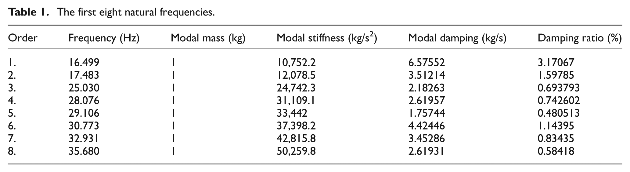
Based on the EMA theory, using PRCE method, the process of modal parameter identification is shown in Figure 11. During modal trials, error was inevitable. Exciting force should inspire each mode, but too high exciting force would cause local nonlinear. Due to the large volume of truck cab, the high frequencies above 100 Hz can be detected rarely. The average of all the transfer functions was computed to get the transfer function set. And the set was processed by the determination of the order to identify the number of modes. The result was shown in Figure 10 with adapting the curve of figure in order to show the peak clearly. Finally, 28 step modes were collected. Using the method of complex modal, single degree to fit the natural modal, and adopting mass normalization method³⁸ (modal mass is defined as 1) to obtain the vibration mode, all results were described in Table 1 and Figure 12.

Figure 11.

Identification flow chart for modal parameter.

Table 1.

The first eight natural frequencies.

Order	Frequency (Hz)	Modal mass (kg)	Modal stiffness (kg/s²)	Modal damping (kg/s)	Damping ratio (%)
1.	16.499	1	10,752.2	6.57552	3.17067
2.	17.483	1	12,078.5	3.51214	1.59785
3.	25.030	1	24,742.3	2.18263	0.693793
4.	28.076	1	31,109.1	2.61957	0.742602
5.	29.106	1	33,442	1.75744	0.480513
6.	30.773	1	37,398.2	4.42446	1.14395
7.	32.931	1	42,815.8	3.45286	0.83435
8.	35.680	1	50,259.8	2.61931	0.58418

Figure 12.

The first eight mode shapes: (a) the first torsional mode along X axis (F = 16.499 Hz), (b) swing and torsion mode along X axis (F = 17.483 Hz), (c) local mode in rear side plate (F = 25.030 Hz), (d) local mode in rear roof panel (F = 28.076 Hz), (e) torsional mode along Y axis and local modes in rear roof panel and the left side plate (F = 29.106 Hz), (f) torsional mode along the Y axis and local mode in roof panel (F = 30.773 Hz), (g) first-order bending vibration around Z axis (F = 30.773 Hz), and (h) mode of rear end of floorboard (F = 35.680 Hz).

In the modal test, there were many local modes described in Table 2.

Table 2.

Local modes of cab.

Frequency	On the top of side plate	In the right rear of floorboard	In the middle of floorboard	In the rear of roof skylight	In front of roof skylight	In the left of rear side plate
F1 (Hz)	25.0340	35.6798	47.3361	28.0706	77.9323	46.7037
F2 (Hz)	29.1046	39.2777	–	29.1046	–	47.3361
F3 (Hz)	46.7037	59.4272	–	30.7763	–	–
F4 (Hz)	50.7271	63.2192	–	32.9312	–	–
F5 (Hz)	–	67.0009	–	40.9036	–	–
F6 (Hz)	–	–	–	47.3361	–	–
F7 (Hz)	–	–	–	54.4701	–	–

Establishment of the finite element model

Building the finite element model of the truck cab to do modal simulation, the simulating results are compared with the test. In the process, we should pay attention to the following points:^39,40

To save time and cost of analysis, the model should be simplified with deleting the fillets less than 10 mm in diameter, small abdicating steps, and transition fillets.

The truck body is made of sheet metal by stamping and spot welding, and its thickness is relatively thin, so shell element in size of 20–30 mm is chosen to discrete the cab. In meshing process, we can control the element quality by aspect ratio, warpage, skew, and Jacobian. The finite model consists of quadrilateral elements in 90%.

The truck cab is assembled together by welding, bolts, riveting, and bonding, using the node coupling method to simulate welding spot, beam elements to simulate the bolts, rigid elements to simulate welding seam, and the spring elements to simulate the bonding.

The cab material is low-carbon steel, the elasticity modulus is 2.1 × 10⁵ MPa, the ratio of Poisson is 0.3, and density is 7.8 × 10³ Kg/m³, adopting isotropic material in simulation.

The finite element model of truck cab shown in Figure 13 includes 211,026 elements and 223,851 nodes. There is 203,212 shell elements, which contain 192,345 quadrilateral elements and 10,867 triangular elements. There are 2152 connecting elements, among them 1389 are rigid elements, 413 are beam elements, and 123 are spring elements.

Figure 13.

Finite element model of truck cab.

Comparison analysis between simulation and test results

Results contrast

The simulation and test results were analyzed, as shown in Table 3.

Table 3.

Comparison between simulation and test modal results.

Order	Simulation results (Hz)	Test results (Hz)	Relative error (%)	Modes description
				FEM	Test
1.	16.135	16.499	2.21	The first torsional mode along X axis
2.	17.324	17.483	0.91	Swing and torsion mode along X axis
3.	24.778	25.030	1.01	Local mode in rear side plate
4.	26.897	28.076	4.12	Local mode in rear roof panel
5.	28.010	29.106	3.76	Torsional mode along Y axis, local modes in rear roof panel and the left side plate
6.	29.512	30.773	4.10	Torsional mode along the Y axis, local mode in roof panel
7.	33.821	32.931	2.70	The first-order bending vibration around Z axis
8.	35.114	35.680	1.59	The mode of rear end of floorboard

FEM: finite element method

From Table 3, the relative error between simulation and experiment results is less than 5%, so the simulation modes are consistent with the test measured. Therefore, the results of simulation and test are reliable.

Improvements of cab

The low-order modes less than 100 Hz of the truck cab are gained in test and simulation. Combined with the actual condition, some suggestions for improvement are proposed as follows.

Figure 14 shows the local mode in left center of rear side along x direction. We suggest that position 1 pointed by arrow in rear part should be stamped into position 2 pointed by arrow, or glued, to prevent vibration and noise.

Figure 14.

The rear wall of cab.

From Figure 15, the vertical beams in both sides of roof also exist the local mode, so the vertical beams and the roof sides should be bonded together using foam.

Figure 15.

Side panels of cab.

Owing to substandard quality of welding or lack of local stiffness, the local mode exists also in the right rear part of the floorboard (location 2 pointed by arrow in Figure 16). Position 1 in left front floor has an elliptical hole compared with the right symmetrical position, and it will result in insufficient stiffness and local modal, so the floorboard around hole should be stamped into flute type.

Figure 16.

Floorboard of cab.

According to Figure 17, the local mode is intensive in rear roof and roof beam, and its frequency is relatively low, so it is easy to generate modal coupling with passenger compartment and cause the resonate noise. The roof pointed by arrow should be stamped into wavy stripes along X axis or glue. In addition, the local mode is relatively obvious in the rear of floor, and it may be related to the large opening at the bottom, hence more attention must be paid to improvements.

Figure 17.

Roof of cab.

Conclusion

The dynamic characteristics of a truck cab are identified using experiments and simulation methods in this article. Modal test scheme is constructed, and the finite element model of the cab is established. Below 100 Hz, 28 step modes are extracted and the test and FEM simulation results are consistent according to comparison. The following observation can be made from the study:

The natural frequencies and modal shapes obtained from experiment and simulation are almost close to each other, so the modal test plan and simulation model are reliable, and this article provides the important design basis to improve truck cab.

The first frequency of truck body should not be equal or close to the external excitation frequencies. The external excitations mainly come from road, engine, transmission, and wheel, and among these incentives, the effect of engine is greatest. Based on the formula of excitation frequency,⁴¹ the engine idling rotational frequency of truck is about 12.5 Hz. To avoid resonance, the first modal frequency should be different from the excitation frequency at least 2 Hz, so it should be larger than 14.5 Hz. As shown in Table 1, the first-order frequency is 16.5 Hz, so the truck will not resonate and the truck body structure is reasonable.

The first torsional mode and the first bending mode have the greatest impact on the truck body; therefore, in order to avoid coupling, the difference between them must be more than 3 Hz. From Table 1, the first torsional vibration frequency is 16.5 Hz, and the first bending frequency is 32.9 Hz, without coupling.

In the process of test and simulation, there are many local modes, and they are most likely caused by unreasonable local structure, low-quality welding, or insufficient local stiffness, such as in left center of rear side along x direction, in the vertical beams, on both sides of roof, and on the right rear part of the floorboard. Those local modes tend to generate modal coupling with passenger compartment and cause the resonate noise, so those positions should be paid more attention in the future improvements.

Footnotes

Acknowledgements

The authors owe a special thank you to Song Shaofang for her suggestions and insights on test.

Academic Editor: Sandra Velarde-Suáre

Declaration of conflicting interests

The authors declare that there is no conflict of interest.

Funding

This work was supported by the Project of National Natural Science Foundation of China (Grant no. 51175320), and partly supported by the Program for Professor of Special Appointment (Eastern Scholar) at Shanghai Institutions of Higher Learning and the Fund for Talents Development by the Shanghai Municipality, China.

References

Yang

. Market and product analysis of heavy truck. Automob Parts 2014; 4: 25–27.

Ding

. Modal study of the cab body in white of a heavy truck. Master’s Thesis, Hunan University, Changsha, China, 2011.

Chen

Lin

. Theoretical and experimental modal analysis of the Guangzhou New TV Tower. Eng Struct 2011; 33(12): 3628–3646.

Mundo

Hadjit

Donders

. Simplified modeling of joints and beam-like structures for BIW optimization in a concept phase of the vehicle design process. Finite Elem Anal Des 2009; 45(4): 452–456.

Zhang

. Dynamic characteristic of the vibratory roller test-bed vibration isolation system: simulation and experiment. J Terramech 2014; 56: 139–156.

Kim

Stubbs

Park

. A new method to extract modal parameters using output-only response. J Sound Vib 2005; 282(1): 215–230.

Ibrahim

Mikulcik

. A method for the direct identification of vibration parameters from the free response. Shock Vib Bull 1977; 4: 183–198.

Cole

Henry

. On the line analysis of random vibrations. In: AIAA/ASME 9th structural dynamics and materials conference, Palm Springs, CA, 1–3 April 1968, pp.288–319. New York, NY: American Institute of Aeronautics and Astronautics.

Cole

. Online failure detection and damping measurement of aerospace structures by random decrement signatures. Washington, DC: National Aeronautics and Space Administration, 1973.

10.

Ibrahim

. Random decrement technique for modal identification of structures. J Spacecraft Rockets 1977; 14(11): 696–700.

11.

Ding

Zhang

Han

. Modeling and modal analysis of multi-body truck system fitted with hydraulically interconnected suspension. J Mech Eng 2012; 48(6): 116–123.

12.

Box

GEP

Jenkins

Reinsel

. Time series analysis: forecasting and control. Hoboken, NJ: John Wiley & Sons, 1994.

13.

Rodrigues

. Modal analysis from ambient vibration survey of bridges: LNEC experience. Studies 1999; 5(7): 81.

14.

Uruzola

Suescun

Celigueta

. Integration of multibody systems in mechatronic simulation environments of any kind. Int J Vehicle Des 2002; 28(1): 57–67.

15.

Brown

Allemang

Zimmerman

. Parameter estimation techniques for modal analysis. SAE technical paper 790221, 1979.

16.

. Modal analysis of body-in-white of multi-purpose vehicle car based on HyperWorks. J Vib Measurement Diagn 2012; 32(1): 138–140.

17.

Van der Auweraer

Guillaume

Verboven

. Application of a fast-stabilizing frequency domain parameter estimation method. J Dyn Syst Meas Contr 2001; 123(4): 651–658.

18.

Verboven

. Frequency domain system identification for modal analysis. Brussels: Vrije Universiteit Brussel, 2002.

19.

Leuridan

Vold

. A time domain linear model estimation technique for multiple input modal analysis. In: Chu

DFH

(ed.) Modal testing and model refinement. New York: American Society of Mechanical Engineers, 1983, pp.51–62.

20.

Vold

Kundrat

Rocklin

. A multi-input modal estimation algorithm for mini-computers. SAE technical paper 820194, 1982.

21.

Zhu

. Modal analysis of a car BIW. J Vib Shock 2013; 32(21): 214–218.

22.

Zhang

Liu

. Structure-borne noise prediction and panel acoustic contribution analysis of a heavy-duty truck cab. J Vib Shock 2014; 33(13): 67–71.

23.

. Design trends of foreign commercial truck cab. Heavy Truck 2013; 3: 38–40.

24.

Ebrahimi

Esfahanian

Ziaei-Rad

. Vibration modeling and modification of cutting platform in a harvest combine by means of operational modal analysis (OMA). Measurement 2013; 46(10): 3959–3967.

25.

Hua

. The modal analysis theory and application. Shanghai, China: Shanghai Jiao Tong University Press, 2000.

26.

Hung

Huang

. Hybrid holographic-numerical method for modal analysis of complex structures. Opt Laser Technol 2010; 42(1): 237–242.

27.

Wang

Cheng

. Modal analysis of mdof system by using free vibration response data only. J Sound Vib 2008; 311(3): 737–755.

28.

Heylen

Sas

. Modal analysis theory and testing. Leuven: Departement Werktuigkunde, Katholieke Universiteit Leuven, 2006.

29.

Heylen

Lammens

Sas

. Modal analysis theory and testing. Beijing, China: Beijing University of Technology Press, 2001 (in Chinese).

30.

Zhou

Fan

Chen

. Modal analysis for body-in-white of a mini bus. Automot Eng 2004; 26(1): 78–80.

31.

Zhang

Chen

. Experimental study on multi work conditions operational modal of automotive engine mounting system. China Mech Eng 2013; 24(22): 3118–3123.

32.

Jin

Peng

. The research for the modal test methods of car’s body-in-white. Automob Technol 2009; 8: 39–43.

33.

LMS International, LMS Test.Lab Rev. 12A user manual. Belgium: LMS International, 2012.

34.

Ferraz

Cherman

De Abreu

. Experimental modal analysis on automotive development. SAE technical paper series, 2003.

35.

Fichera

Lacagnina

Petrone

. Modeling of torsion beam rear suspension by using multibody method. Multibody Syst Dyn 2004; 12(4): 303–316.

36.

Møller

Gade

. Application of operational modal analysis on cars. In: Noise and vibration conference and exhibition, 2003, pp.1970–1977; SAE technical paper 2003-01-1599.

37.

Dev

VMSS

Angadi

Roy

. Forming and modal analysis of sheet metal oil pan. Innovations 2002; 1: 0716.

38.

Parloo

Cauberghea

Benedettini

. Sensitivity-based operational mode shape normalization: application to a bridge. Mech Syst Signal Process 2005; 19(1): 43–55.

39.

Zuo

. A complete development process of finite element software for body-in-white structure with semi-rigid beams in .NET framework. Adv Eng Softw 2012; 45(1): 261–271.

40.

Altunisik

Bayraktar

Sevim

. Operational modal analysis of a scaled bridge model using EFDD and SSI methods. Indian J Eng Mater Sci 2012; 19: 320–330.

41.

Automotive Engineering Handbook Editorial Committee. Automotive engineering handbook-tests section. Beijing, China: China Communications Press, 2001.

Modal analysis of a truck cab using the least squares complex exponent test method

Abstract

Keywords

Introduction

Theory of modal analysis

Modal test of truck cab

Theory of modal test

Establishment of the test system

Composition of the test system

Experiment scheme

Collection of experiment data

Data processing

Response frequency and vibration modes

Establishment of the finite element model

Comparison analysis between simulation and test results

Results contrast

Improvements of cab

Conclusion

Footnotes

Acknowledgements

Declaration of conflicting interests

Funding

References