
Abstract
The controlled motion of a rigid body in the horizontal plane is investigated in this article. Three internal and acceleration-controlled masses are used to actuate the system. Dry friction acting between the system and the plane is isotropic. The dynamics of two basic motions of the system, that is, rectilinear and rotary motions, are first studied. Then by combining these two basic types of motions, planar locomotion of the system is constructed. Two typical planar trajectories of the system, that is, oblique lines and curve lines, are proposed and both approached with folding lines. The slope of the oblique lines and the curvature of the curves can be adjusted by varying the drive parameters, and the planar locomotion is thus controlled. To achieve a maximum average velocity, the drive parameters are optimized.
Introduction
With the rapid development of robot applications, micro-robots are attracting more and more attention of worldwide researchers. The reason lies in the huge potential of micro-robots in applications of pipeline inspection, earthquake rescue, medicine delivery, precision positioning, and so on. Conventional robots have outer components like legs, wheels and caterpillars, and complex transmission gears, which make it hard for them to be miniaturized. In contrast, vibration-driven systems are driven by the periodic motions of their internal masses. They are simple in design and easy to be manufactured in miniature size. In addition, their hermetic shapes make them adaptable to many extreme resistive media with high viscidity or corrosivity.
Chernous’ko, Bolotnik, Fang, and Xu have carried out intensive researches on the rectilinear motion of vibration-driven systems with one internal mass.1–6 The vibration-driven system1–4 is composed of a rigid body and one internal mass. The mass moves periodically inside the rigid body. Due to the anisotropic dry friction acting on the body by supporting plane, the system has a net displacement in each period. Two modes of the piecewise constant drives, that is, two-phase mode and three-phase mode, are applied to the internal mass. With the two-phase mode, Chernous’ko analyzed and optimized the rectilinear motion of the vibration-driven system subjected to dry friction, linear, and quadratic resistance. It is shown that for the isotropic quadratic resistance, the system performs progressive motion, while for the linear resistance it can only have net displacement in the medium with anisotropic resistance. Rectilinear motion of the vibration-driven system in three-phase mode is investigated in Chernous’ko 1 and Fang and Xu. 5 In Fang and Xu, 5 the method of averaging is utilized to analyze the steady state motion, and stick-slip effect is taken into account. The drive forms of vibration-driven systems still have many other types, for example, harmonic drive.6–8 Fang and Xu 6 investigated the rectilinear motion of the vibration-driven system in the presence of anisotropic dry friction. Their focus is on the stick-slip effect of the rectilinear motion, and the diagram of sliding bifurcation is analytically presented. Bolotnik and colleagues7,8 greatly improved the rectilinear motion of the vibration-driven system by optimizing the harmonic motions of two internal masses. Moreover, robots like inverted pendulum 9 and mini-robots 10 verified the theory of the vibration-driven system and exhibited the potential of the system in miniaturization.
In order to realize planar locomotion, more internal drive components (translational or rotating masses) are added to vibration-driven systems. A vibration-driven system with four short legs is modeled by Volkova and Yatsun. 11 The system is actuated by the harmonic motions of two internal masses, which are restricted within two paralleled straight guides. An algorithm is proposed to approximate the “S” shape curve trajectory. In Vartholomeos and colleagues,12–14 the planar trajectory of the vibration-driven system is controlled by three rotating masses with high accuracy. Additionally, the system is low in cost and energy supply. The layouts of the internal masses in the above system are symmetric. Besides, inphase and antiphase motions are performed by the internal masses to control the planar trajectories.
Based on the analysis and optimization of a box-like rigid body with one internal mass in Chernous’ko, 1 we introduce two more internal masses and extend to the study of the planar locomotion of the updated system. Two basic types of motions, that is, rectilinear motion and rotary motion, are proposed to construct the planar locomotion of the system. As a result, planar trajectories of the system are approximately provided.
Dynamics of the mechanical system
Description of the dynamic system
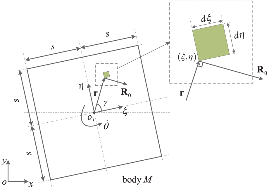
The vibration-driven system under consideration is a cuboid (called body M) with square top and bottom, which is placed in a horizontal plane (see Figure 1). Inside the body, three masses m
1, m
2, and m
3 are mounted to the square bottom. On the bottom, coordinate frame
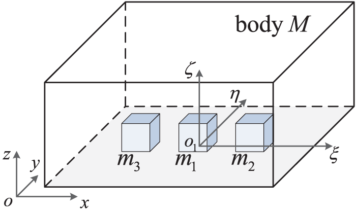
Scheme of the vibration-driven system.

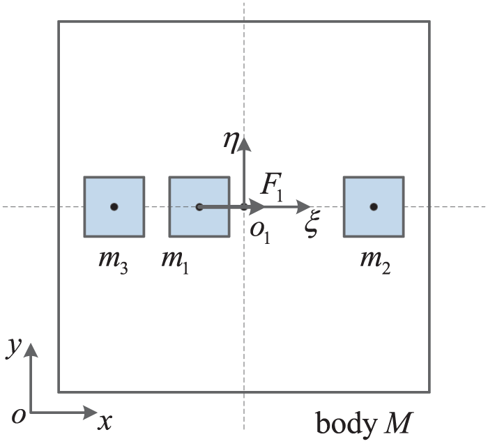
Layouts of the dynamic system.
Rectilinear and rotary motions
Rectilinear motions
Rectilinear motion of body M due to the motion of single mass m 1
In this scenario, mass m
1 moves periodically along the axis

Rectilinear motion of body M with single mass m 1 moving.
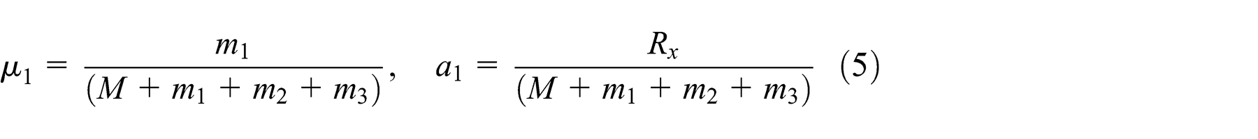
where M, m 1, m 2, and m 3 are the mass of body M, masses m 1, m 2, and m 3, respectively; F 1 is the force acted on body M by mass m 1; and Rx is the dry friction acted by the supporting plane, which is defined as

and for

where f is the dry friction coefficient and g is the gravitational acceleration. Eliminating F 1 in equation (1) yields

where
2. Rectilinear motion of body M due to the inphase motions of masses m 2 and m 3
Now masses m
2 and m
3 perform inphase motions parallel to the axis


Rectilinear motion of body M with the inphase motions of masses m 2 and m 3.
Due to the symmetry of masses m 1 and m 2, one has

Assuming

we obtain

The directions of position vectors
Thus, the governing equations of body M in this scenario are given by
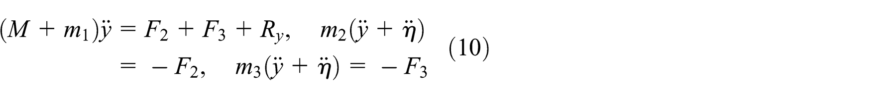
where dry friction Ry is defined as

and for

Eliminating F 2 and F 3 in equation (10) yields

where
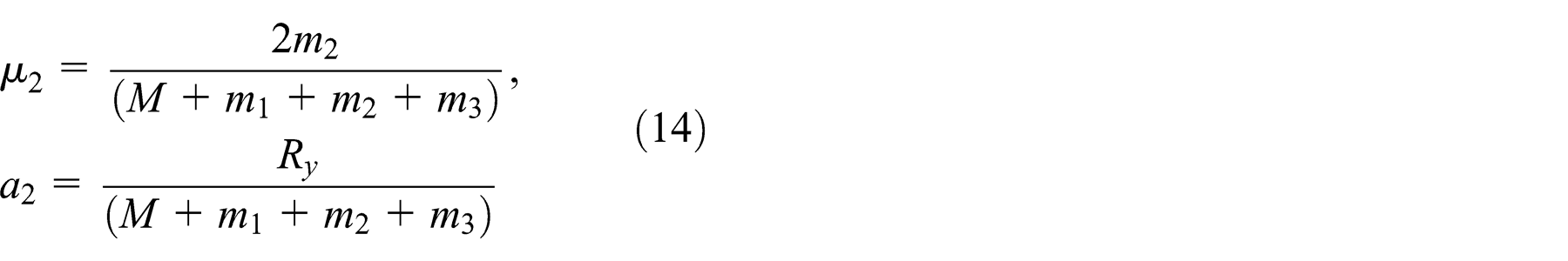
Letting

we obtain
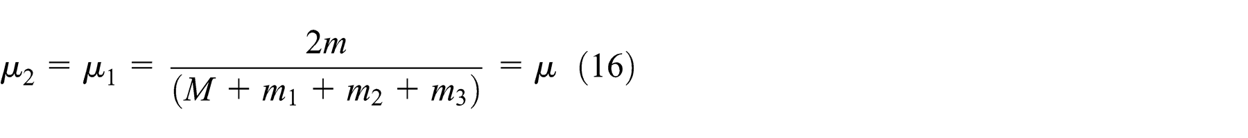
Comparing equations (4) and (13), we represent them with

where

Up to now, the first basic type of body M’s motion is presented. From equation (17), one may find that rectilinear motions in the x- and y-directions have no differences although they are realized through different internal motions. In the next section, we will see how the rotary motion is constructed.
Rotary motion
To achieve a rotary motion of body M, masses m
2 and m
3 are expected to perform antiphase motions parallel to the axis

Rotary motion of body M with the antiphase motions of masses m 2 and m 3.
Due to the antisymmetry of masses m 2 and m 3, one has

Consequently

from which one may know that in this scenario, body M simply rotates about its center o 1 without translation.
To set up the governing equation of the rotation of body M, first, we need to acquire the total kinetic energy of the system. In Figure 5, the relative position vectors are

Then, the absolute position vectors of masses m 2 and m 3, are, respectively, given by

where the transformation matrix

The total kinetic energy T of the system can be given as

where the dots denote the derivative with respect to time t, and Jm is the sum of rotational inertias of all components of the system with respect to their own centers.
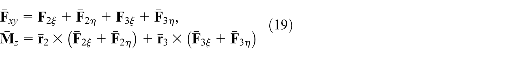
Utilizing the Lagrange equation of the second kind

in which

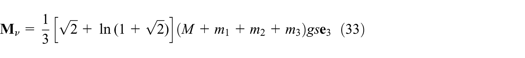
Here, some remarks on the rotary resistance

Analysis of the friction acting on body M when it rotates.
where

where s is half of the side length of the square bottom and

of the point

and

Similarly, if body M rotates clockwise, we obtain that
Denoting

we summarize that
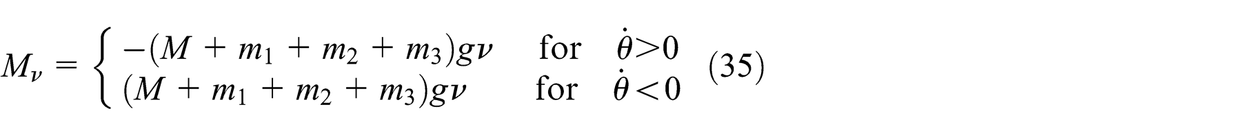
For

From equations (35) and (36), one may find that
To obtain the angular velocity

where t 0 denotes the initial moment. It is easy to see from equation (37) that

Up to now, governing equations of the two basic types of body M’s motion are established. It is also known to us that vibration-driven systems move due to the vibrations of some components of their own. However, variables
Internal acceleration-controlled motion
In order to actuate body M, internal masses m 1, m 2, and m 3 are assumed to move periodically within it. Relative displacements of them are constrained in a prescribed length L given by

Moreover, relative accelerations, velocities, and displacements of the internal masses are periodic functions with the same period Ti
. At the initial moment of each period, the internal masses are supposed to be at rest in their initial positions, and they reach the maximum relative displacements L at

and

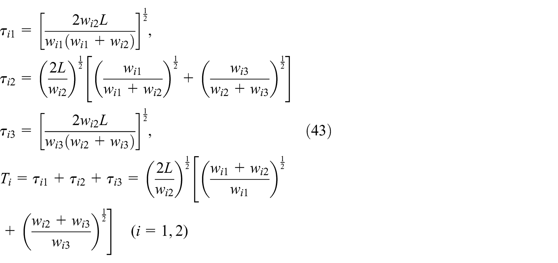
Here, we introduce the drive mode of the internal masses (see Figure 7). The drive mode is divided into three segments and the length of each segment is denoted as


Acceleration-controlled mode of the internal masses: (a) relative acceleration of the internal masses during one period, (b) relative velocity of the internal masses during one period, and (c) relative displacement of the internal masses during one period.
With some calculations, we represent
In practical application, there should be constraints on the relative accelerations of internal masses, thus

Furthermore, to actuate the system, the maximum drive force and moment should exceed the resistances; thus, it can be derived from equations (17) and (27) that

By integrating equation (42), we obtain the relative velocity of internal masses (see Figure 7(b))
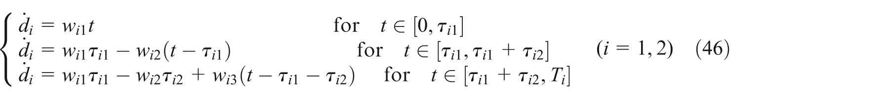
and the relative displacement (see Figure 7(c))
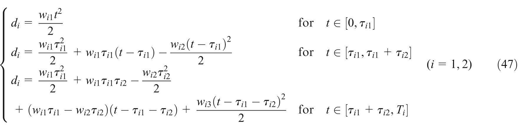
For the excitation shown in equation (42), the rectilinear or rotary motion of body M may have two modes, that is, modes a and b (see Figure 8). In mode a, the velocity of body M is negative at first, then turns positive, and finally decreases to 0 until the end of this period. In mode b, the velocity of body M has only positive value. After reaching a peak, it vanishes and keeps at 0 until the end of the period. For a more natural, simple, and convenient practical realization, only mode b is considered in this article.

Two motion modes of body M under the acceleration-controlled mode: (a) mode a and (b) mode b.
For the rectilinear motion in the x- or y-direction, substituting equation (42) into equation (17) and integrating equation (17) for mode b yield

where
To ensure mode b, it needs to be satisfied that

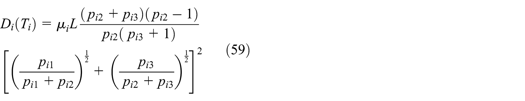
Under this constraint, we can calculate the rectilinear displacement of body M as

and the average rectilinear velocity of body M as

For the rotary motion in the

where

Correspondingly, we calculate the rotary displacement of body M in one period as

and the average rotary velocity of body M in one period as

For further optimization, we introduce the dimensionless variables as
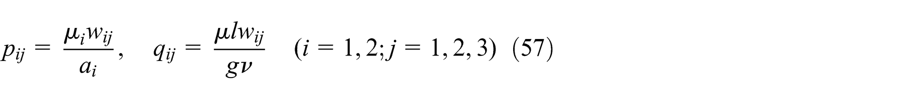
With them, we change equations (50), (51), (52), (54), (55), and (56) into dimensionless forms, given by


Based on these nondimensionalized equations, the planar locomotion on body M is constructed in the next section.
Planar locomotion and optimized drive mode
If the trajectory of a system is planar, then we consider its motion to be planar motion. In this section, we classify the planar trajectories into two kinds of lines, that is, oblique lines and curve lines. The trajectory of the planar locomotion constructed is composed of these two kinds of lines. However, it is hard or even impossible for a vibration-driven system to move exactly along an oblique line or a curve line, so we use folding lines to approach the two kinds of lines along which body M is expected to move. In the process, the motion of body M in one period is divided into two stages. In each stage, one type of the two basic motions of body M, that is, rectilinear motion and rotary motion, is chosen. Thus, with different combinations of the basic motions, the trajectory of body M may be different folding lines. In this way, planar trajectories of body M in oblique lines or curve lines are approximated. To this end, we start from the oblique lines.
Oblique lines
Construction of the oblique lines
To approach oblique lines, we design the relative accelerations of internal masses as shown in Figure 9. In the first stage, mass m
1 moves alone, while in the second stage masses m
2 and m
3 perform inphase motions spontaneously. The motions in the first and second stages are governed by equations (4) and (13), respectively. The displacements of body M in one period

Acceleration-controlled mode for oblique lines.

Trajectory of body M in one period designed to approach oblique lines.
Slope of oblique lines
From the former discussion, one knows that the route AB plus BC is equivalent to the route AC, which is an oblique line. The slope k of AC is given as

It is to see that by changing the sign of the drive modes or reversing the order of the two stages, one can control body M to move along oblique lines with different slopes. Then, it is sufficient to study the oblique lines with the slope

Substituting equation (64) into equation (65) yields

Thus, to achieve a maximum average velocity, it is assumed that body M moves with the optimized drive parameters
Considering equation (58), we choose that

Substituting equation (68) into equation (59) yields
and it follows from equation (64) that

To optimize the motion in the second stage, we choose

Substituting equations (70) and (71) into equation (59) yields

from which it can be solved that

Letting k = 1 in equation (73), we can see that
Curve lines with rectilinear and rotary motions
Construction of the curve lines
As for the curve lines, we design the relative accelerations of internal masses as shown in Figure 11. In the first stage, mass m
1 moves alone, while in the second stage masses m
2 and m
3 perform antiphase motions spontaneously. Equations (4) and (27) govern the motions in the first and second stages, respectively. The displacements of body M in one period

Acceleration-controlled mode for curve lines.

Trajectory of body M in one period designed to approach curve lines.
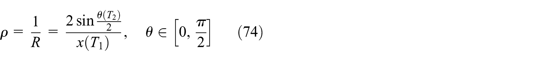
Curvature of the curve lines
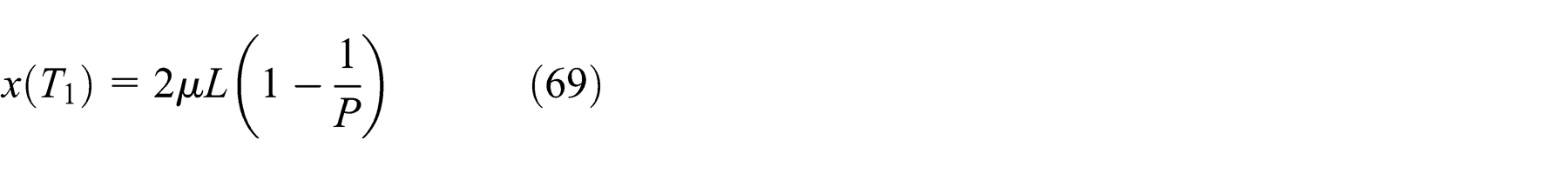
From the discussion above, we know that points E, F, and G are on the circumcircle with radius R. After some geometric processing, the curvature of the curve line is represented as
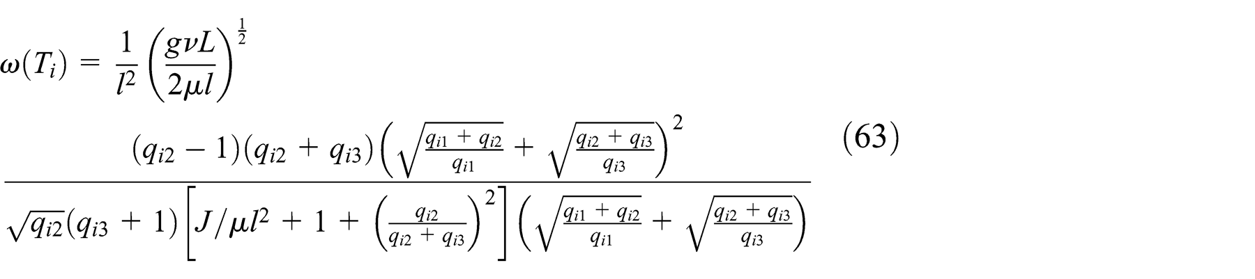
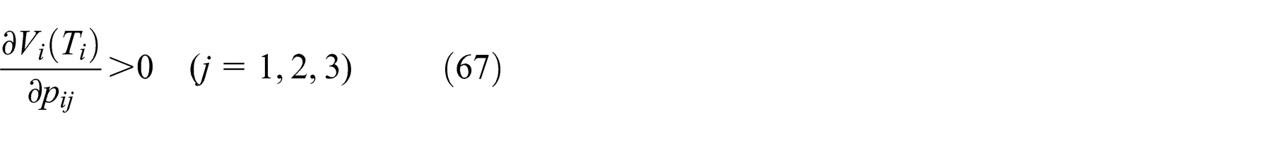
To achieve a maximum velocity, it is also assumed that the rectilinear motion in the first stage is optimized. The drive parameters are chosen as displayed in equation (68). For the second stage, we calculate the partial derivatives of
Considering equation (61), we choose

Substituting equations (62), (69), and (76) into equation (74) yields
from which one may obtain that

where

By solving equation (78), one may obtain dimensionless drive parameter
Up to now, the drive parameters of the second pattern of motion are determined, that is, according to equations (68), (76), and (78), body M can move roughly along curves with given curvature
Conclusions
A vibration-driven system with three internal and acceleration-controlled masses is modeled to perform the planar locomotion. With the inphase and antiphase motions of the internal masses, the system can move in a straight line or rotate about its center, respectively. The two basic types of motions are utilized to construct the planar motion of the vibration-driven system.
Two typical trajectories of the dynamic system, that is, oblique lines and curve lines, are considered in the article. For the oblique lines, we construct them by alternating rectilinear motions of body M in the x- and y-directions. For the curve lines, body M is controlled to have a linear displacement followed with an angular displacement in each period. As a result, both the planar lines are approached by folding lines. Assuming that the displacements of body M in the two basic motions are not very large or even tiny, the actual trajectory of the dynamic system is close enough to the oblique and curve lines.
Two characteristic parameters of body M’s trajectories, that is, the slope of the oblique lines and the curvature of the curve lines, are defined and expressed in the drive parameters wij (i = 1, 2; j = 1, 2, 3). The planar trajectory changes with the drive parameters varying. Thus, one can construct planar trajectories of body M with different slopes or curvatures.
To achieve a maximum velocity of the system, drive parameters wij (i = 1, 2; j = 1, 2, 3) are both optimized for rectilinear and rotary motion. We find that the velocities of rectilinear and rotary motions both grow monotonically with the increase in the drive parameters wi 1 and wi 3. Thus, in the optimized motions, wi 1 and wi 3 take their maximum values while wi 2 is utilized to control the geometric shape of the folding lines.
Footnotes
Academic Editor: Fen Wu
Declaration of conflicting interests
The authors declare that there is no conflict of interest.
Funding
This research was supported by National Natural Science Foundation of China under Grant No. 11272236.