Sage Journals: Discover world-class research

Abstract

A three-dimensional model was developed to simulate the heat transfer rate on a heat pipe in a transient condition. This article presents the details of a calculation domain consisting of a wall, a wick, and a vapor core. The governing equation based on the shape of the pipe was numerically simulated using the finite element method. The developed three-dimensional model attempted to predict the transient temperature, the velocity, and the heat transfer rate profiles at any domain. The values obtained from the model calculation were then compared with the actual results from the experiments. The experiment showed that the time required to attain a steady state (where transient temperature is constant) was reasonably consistent with the model. The working fluid r134a (tetrafluoroethane) was the quickest to reach the steady state and transferred the greatest amount of heat.

Keywords

Heat pipe transient condition three-dimensional working fluid heat transfer

Introduction

A heat pipe with an internal wick was studied in this research. As part of the research, the design of the heat pipe and variable conductance devices for spacecraft thermal control was evaluated. During the analysis, subjects that were considered include hydrostatics, hydrodynamics and heat transfer into and out of the pipe, fluid selection, material compatibility, and variable conductance of a heat pipe.¹ Heat pipes are heat transfer devices which can be modeled numerically and analytically to predict their own heat transfer effectiveness. Vlassov and Riehl present a mathematical model of a loop heat pipe (LHP), which has been validated with experimental results. The LHP behavior was then predicted as a thermal control component of a satellite under different scenarios of orbital heat fluxes impression on the condenser–radiator.² Nemec et al. have created a mathematical model in MS Excel for computing relations of heat transfer limitations, which define the boundaries of heat pipe performance. The limitation values depend on heat pipe parameters, wick structure parameters, and the thermophysical properties of the working fluid.³ Tournier and El-Genk⁴ developed a model for heat pipe analysis to predict the transient values of the vapor and wall temperatures as well as the effective power throughput, which are in reasonable agreement with experiments. Jang et al. suggested that the numerical results are obtained using the finite difference method. They were able to achieve a good comparison of the transient results for the simulated heat pipe vapor flow with the two-dimensional model, and the steady-state results were in agreement with existing experimental data.⁵ Modeling is often used to predict the performance of heat pipes. Performance analysis including the concept of temperature distribution, frozen start-up behavior of a heat pipe, and an equation for analyzing temperature distribution of the heat pipe wall⁶ are part of the modeling process. The effect of different parameters, such as wall thermal conductivity, wick porosity, and heat pipe dimensions on heat pipe operation, was also considered. A transient model for a micro-grooved heat pipe of any polygonal shape was presented using a macroscopic approach as reported by Suman et al.⁷ A transient, three-dimensional model for thermal transport in heat pipes and vapor chambers was developed by Ranjan et al. They used the Navier–Stokes equations along with the energy equation to determine the liquid and vapor flows numerically. A porous medium formulation was used for the wick region. Evaporation and condensation at the liquid–vapor interface were modeled using kinetic theory. The coupled model is used to predict the performance of a heat pipe with a screen-mesh wick, and the implications of the coupling employed are discussed.⁸ The coupled equations of heat, mass, and momentum transfer were utilized to obtain the transient as well as the steady-state profiles of various parameters—namely, the substrate temperature, the liquid velocity, the liquid pressure, and so on. Choudhary et al.⁹ discovered that wrapping a hydrophilic wick fabric on the cold pipe can significantly reduce the thermal degradation. The model was based on the volume-averaged equations for unsteady transport of heat, water vapor, and liquid water in a porous medium. The wick model also allows for the presence of a vapor retarder jacket that is used to reduce the ingress of water vapor into the insulation. The effects of capillary pressure on the performance of the heat pipe were reported by Thuchayapong et al.¹⁰ They have successfully simulated a two-dimensional numerical simulation of heat transfer and fluid flow in a heat pipe at a steady state using the finite element method. A heat pipe with a wick was studied in this research. As part of this research, the design of the heat pipe and variable conductance devices for spacecraft thermal control were evaluated. The aim of this study was to develop a governing equation in three-dimensional numerical simulation and to predict temperature, velocity, and heat transfer rates using the finite element method. The standard Galerkin approach was selected to solve the governing equation. The temperature profile on the pipe wall and the heat transfer rate were also simulated and compared with the experimental data for each of the three working fluids.

Modeling approach

The heat pipe consists of three parts: evaporator section, adiabatic section, and condenser section which combined make up the total length of the pipe. The heat pipe was used as a heat transfer device with the heat transfer being achieved by a change of phase (latent heat of evaporation) of a working fluid. The schematic diagram and coordinate systems of the heat pipe components including the wall, a wick structure, and a vapor core¹¹ are shown in Figure 1.

Figure 1.

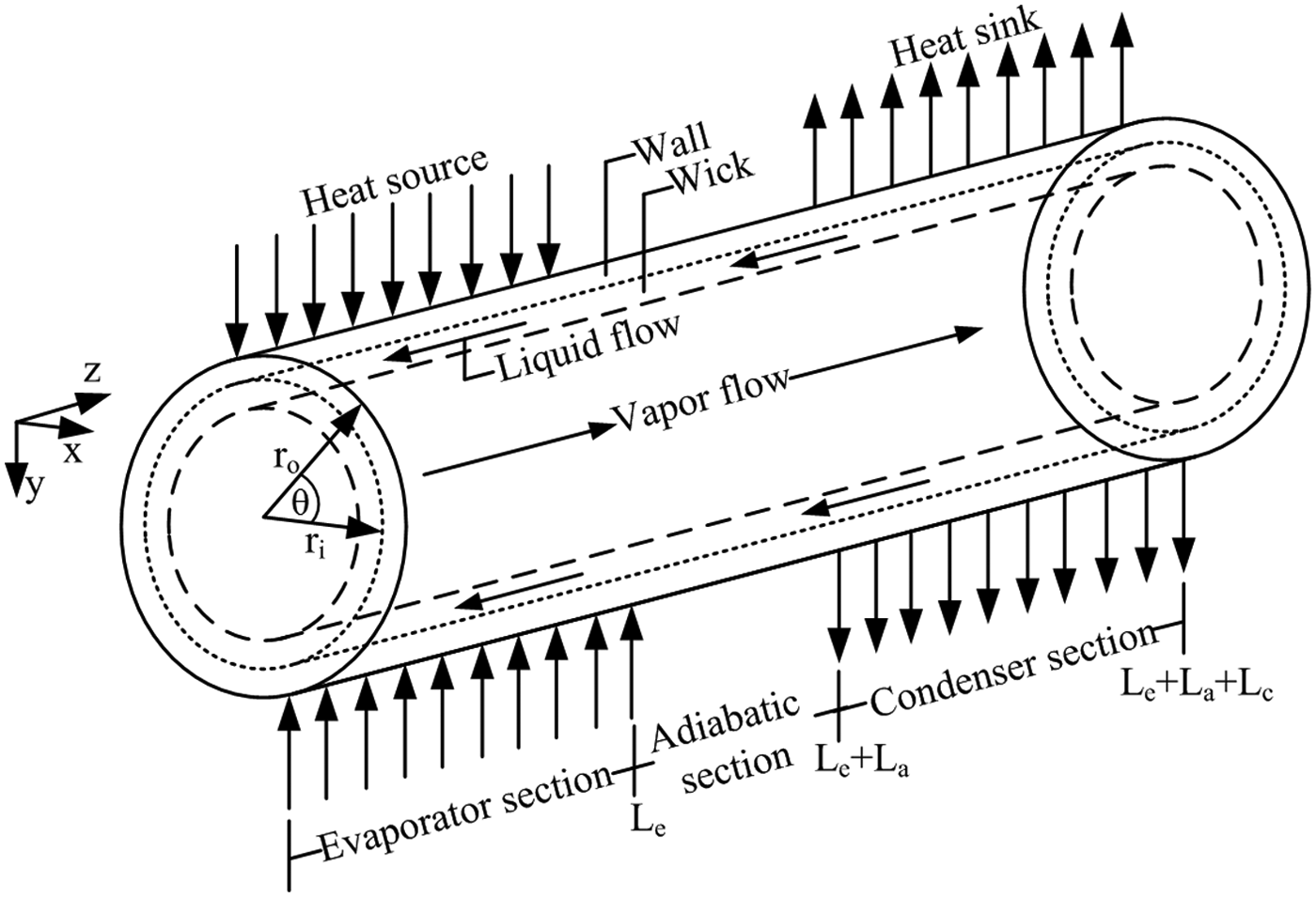
Schematic diagram of the heat pipe with the coordinate system.

Heat conduction of the pipe wall

Under normal operation, the heat applied to the evaporator section by an external source is conducted through the pipe wall. The three-dimensional transient condition heat conduction equation that describes the temperature in the heat pipe wall from conservation of energy is

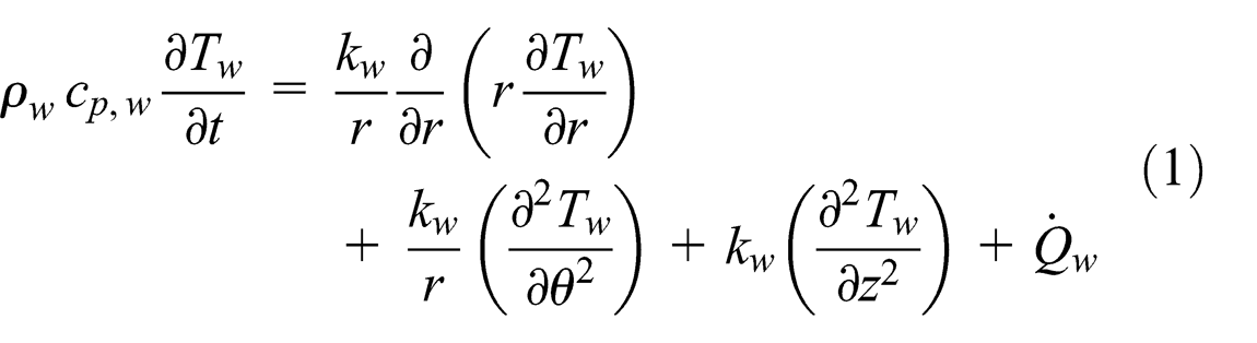
\begin{matrix} ρ_{w} c_{p, w} \frac{\partial T_{w}}{\partial t} = & \frac{k_{w}}{r} \frac{\partial}{\partial r} (r \frac{\partial T_{w}}{\partial r}) \\ + \frac{k_{w}}{r} (\frac{\partial^{2} T_{w}}{\partial θ^{2}}) + k_{w} (\frac{\partial^{2} T_{w}}{\partial z^{2}}) + {\overset{\cdot}{Q}}_{w} \end{matrix}

(1)

where $ρ_{w} c_{p, w}$ is the effective heat capacity of the pipe wall, and $k_{w}$ is the effective thermal conductivity of the pipe wall.

Fluid flow of vapor phase in the vapor core

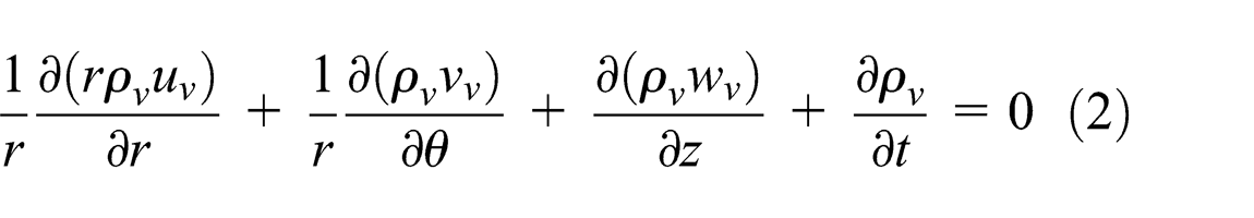
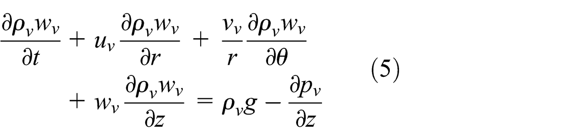
When heat is applied to the evaporator section, the working fluid within the vapor core heats and evaporates. Heat is absorbed by vaporizing the working fluid. The vapor travels to the condenser section driven by the build-up of pressure. In the vapor core section, in order to predict the velocity profile of the vapor phase, the continuity, momentum, and energy balance equations were used as follows

\frac{1}{r} \frac{\partial (r ρ_{v} u_{v})}{\partial r} + \frac{1}{r} \frac{\partial (ρ_{v} v_{v})}{\partial θ} + \frac{\partial (ρ_{v} w_{v})}{\partial z} + \frac{\partial ρ_{v}}{\partial t} = 0

(2)

\begin{matrix} \frac{\partial ρ_{v} u_{v}}{\partial t} & + u_{v} \frac{\partial ρ_{v} u_{v}}{\partial r} + \frac{v_{v}}{r} \frac{\partial ρ_{v} u_{v}}{\partial θ} \\ + w_{v} \frac{\partial ρ_{v} u_{v}}{\partial z} - \frac{ρ_{v} v_{v}^{2}}{r} = ρ_{v} g - \frac{\partial p_{v}}{\partial r} \end{matrix}

(3)

\begin{matrix} \frac{\partial ρ_{v} v_{v}}{\partial t} & + u_{v} \frac{\partial ρ_{v} v_{v}}{\partial r} + \frac{v_{v}}{r} \frac{\partial ρ_{v} v_{v}}{\partial θ} \\ + w_{v} \frac{\partial ρ_{v} v_{v}}{\partial z} - \frac{ρ_{v} u_{v} v_{v}}{r} = ρ_{v} g - \frac{\partial p_{v}}{\partial θ} \end{matrix}

(4)

\begin{matrix} \frac{\partial ρ_{v} w_{v}}{\partial t} & + u_{v} \frac{\partial ρ_{v} w_{v}}{\partial r} + \frac{v_{v}}{r} \frac{\partial ρ_{v} w_{v}}{\partial θ} \\ + w_{v} \frac{\partial ρ_{v} w_{v}}{\partial z} = ρ_{v} g - \frac{\partial p_{v}}{\partial z} \end{matrix}

(5)

\begin{matrix} ρ_{v} c_{p, v} (\frac{\partial T_{v}}{\partial t} + u_{v} \frac{\partial T_{v}}{\partial r} + \frac{v_{v}}{r} \frac{\partial T_{v}}{\partial θ} + w_{v} \frac{\partial T_{v}}{\partial z}) \\ = k_{v} [\frac{1}{r} \frac{\partial}{\partial r} (r \frac{\partial T_{v}}{\partial r}) + \frac{1}{r^{2}} \frac{\partial^{2} T_{v}}{\partial θ^{2}} + \frac{\partial^{2} T_{v}}{\partial z^{2}}] \\ + 2 μ_{v} [{(\frac{\partial u_{v}}{\partial r})}^{2} + {\frac{1}{r} (\frac{\partial v_{v}}{\partial θ} + v_{v})}^{2} + {(\frac{\partial w_{v}}{\partial z})}^{2}] \\ + μ_{v} [{(\frac{\partial v_{v}}{\partial z} + \frac{1}{r} \frac{\partial w_{v}}{θ})}^{2} + {(\frac{\partial w_{v}}{\partial r} + \frac{\partial u_{v}}{\partial z})}^{2} \\ + {(\frac{1}{r} \frac{\partial u_{v}}{\partial θ} + r \frac{\partial}{\partial r} (\frac{v_{v}}{r}))}^{2}] \\ - \frac{2}{3} μ_{v} {(\frac{1}{r} \frac{\partial}{\partial r} (r u_{v}) + \frac{1}{r} \frac{\partial v_{v}}{\partial θ} + \frac{\partial w_{v}}{\partial z})}^{2} \\ + \frac{u_{v} \partial p_{v}}{\partial r} + \frac{v_{v}}{r} \frac{\partial p_{v}}{\partial θ} + w_{v} \frac{\partial p_{v}}{\partial z} \end{matrix}

(6)

Fluid flow of liquid phase in the wick structure

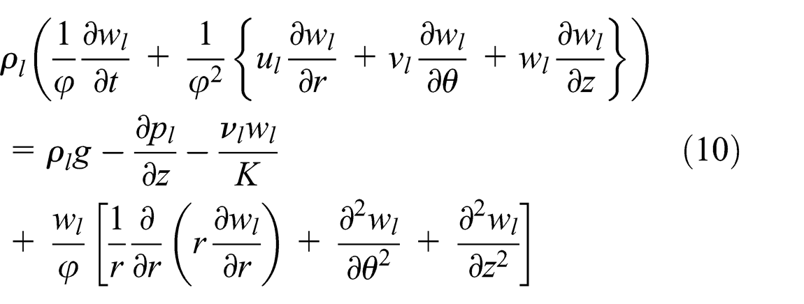
When the vapor moves to the condenser section, it is cooled and turned back to a saturated liquid. The condensed liquid is returned to the evaporator section using a wick structure exerting a capillary action on the liquid phase of the working fluid. Therefore, the velocity profile of the liquid phase in the wick structures using the continuity and momentum equations is as follows

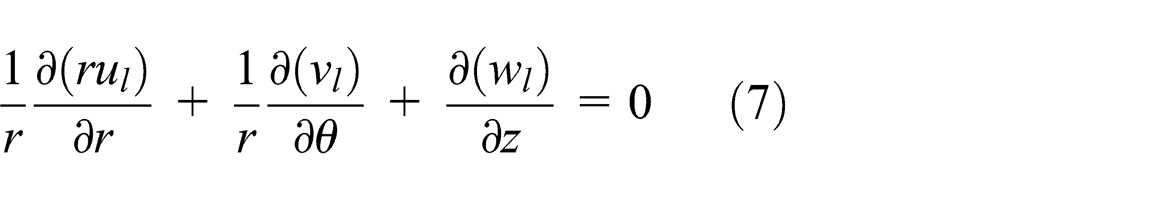
\frac{1}{r} \frac{\partial (r u_{l})}{\partial r} + \frac{1}{r} \frac{\partial (v_{l})}{\partial θ} + \frac{\partial (w_{l})}{\partial z} = 0

(7)

The momentum equation consists of the convective term, body force, and pressure term. The last term applied was Darcy’s law, which is the friction force in the wick, shown in equations (8)–(10)

\begin{matrix} ρ_{l} (\frac{1}{φ} \frac{\partial u_{l}}{\partial t} + \frac{1}{φ^{2}} {u_{l} \frac{\partial u_{l}}{\partial r} + v_{l} \frac{\partial u_{l}}{\partial θ} + w_{l} \frac{\partial u_{l}}{\partial z}}) \\ = ρ_{l} g - \frac{\partial p_{l}}{\partial r} - \frac{ν_{l} u_{l}}{K} \\ + \frac{u_{l}}{φ} [\frac{1}{r} \frac{\partial}{\partial r} (r \frac{\partial u_{l}}{\partial r}) + \frac{1}{r} \frac{\partial^{2} u_{l}}{\partial θ^{2}} - \frac{v_{l}}{r^{2}} + \frac{\partial^{2} u_{l}}{\partial z^{2}}] \end{matrix}

(8)

\begin{matrix} ρ_{l} (\frac{1}{φ} \frac{\partial v_{l}}{\partial t} + \frac{1}{φ^{2}} {u_{l} \frac{\partial v_{l}}{\partial r} + v_{l} \frac{\partial v_{l}}{\partial θ} + w_{l} \frac{\partial v_{l}}{\partial z}}) \\ = ρ_{l} g - \frac{\partial p_{l}}{\partial θ} - \frac{ν_{l} v_{l}}{K} \\ + \frac{v_{l}}{φ} [\frac{1}{r} \frac{\partial}{\partial r} (r \frac{\partial v_{l}}{\partial r}) + \frac{1}{r} \frac{\partial^{2} v_{l}}{\partial θ^{2}} - \frac{u_{l} v_{l}}{r^{2}} + \frac{\partial^{2} v_{l}}{\partial z^{2}}] \end{matrix}

(9)

\begin{matrix} ρ_{l} (\frac{1}{φ} \frac{\partial w_{l}}{\partial t} + \frac{1}{φ^{2}} {u_{l} \frac{\partial w_{l}}{\partial r} + v_{l} \frac{\partial w_{l}}{\partial θ} + w_{l} \frac{\partial w_{l}}{\partial z}}) \\ = ρ_{l} g - \frac{\partial p_{l}}{\partial z} - \frac{ν_{l} w_{l}}{K} \\ + \frac{w_{l}}{φ} [\frac{1}{r} \frac{\partial}{\partial r} (r \frac{\partial w_{l}}{\partial r}) + \frac{\partial^{2} w_{l}}{\partial θ^{2}} + \frac{\partial^{2} w_{l}}{\partial z^{2}}] \end{matrix}

(10)

The porosity of the mesh wick as shown in Figure 2 for $φ$ is defined as follows

φ = 1 - \frac{π AB}{2 (1 + A)} \sqrt{1 + {(\frac{A}{1 + A})}^{2}}

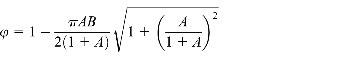
where $A = d / W$ , $B = d / s$ , and s is the thickness of the wick.

Figure 2.

Schematic representation of the mesh wick: (a) top view and (b) cross-sectional A–A.

The energy balance equation explains the law of conservation of energy shown in equation (11). This equation can predict the temperature profile of the liquid phase within the wick structure

\begin{matrix} {(ρ c_{p})}_{eff} (\frac{\partial T_{l}}{\partial t} + u_{l} \frac{\partial T_{l}}{\partial r} + \frac{v_{l}}{r} \frac{\partial T_{l}}{\partial θ} + w_{l} \frac{\partial T_{l}}{\partial z}) \\ = k_{eff} [\frac{1}{r} \frac{\partial}{\partial r} (r \frac{\partial T_{l}}{\partial r}) + \frac{1}{r^{2}} \frac{\partial^{2} T_{l}}{\partial θ^{2}} + \frac{\partial^{2} T_{l}}{\partial z^{2}}] \end{matrix}

(11)

where $k_{eff}$ is effective thermal conductivity of the liquid in the wick as $k_{eff} = k_{l} [(k_{l} + k_{s}) - (1 - φ) (k_{l} - k_{s})] / [(k_{l} + k_{s}) + (1 - φ) (k_{l} - k_{s})]$ , where $k_{l}$ and $k_{s}$ were the thermal conductivity of the working fluid and material wick, respectively.

Heat transfer rate of a heat pipe

The heat transfer rate of the heat pipe was evaluated by calculating the velocity of the vapor to liquid phase change within the condenser section given by equation (12)

{\overset{\cdot}{Q}}_{out} = w_{v} 2 ρ_{v} π r_{v} L_{c} h_{fg}

(12)

where $h_{fg}$ is latent heat of vaporization of working fluid.

Boundary conditions

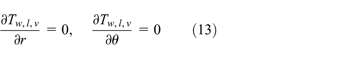
At the wall–wick and wick–vapor interfaces, no heat is transferred to the wick structure or the vapor core during this time, since both ends of the heat pipe are insulated.^12,13 Therefore

\frac{\partial T_{w, l, v}}{\partial r} = 0, \frac{\partial T_{w, l, v}}{\partial θ} = 0

(13)

At the z coordinates, there were three different boundary conditions for the outer wall of the heat pipe. In the evaporator and condenser sections, it is assumed that a constant temperature was supplied during the entire operation, and the heat load is applied to the outer wall surface of the evaporator section. The adiabatic section was insulated, and the heat from the condenser section was continuously exchanged by cooling water, as explained in equation (14)

{\begin{matrix} T_{e} = 60 \circ C 0 \leq z < L_{e} \\ \frac{\partial T_{a}}{\partial z} = 0 L_{e} \leq z < L_{e} + L_{a} \\ T_{c} = 20 \circ C L_{e} + L_{a} \leq z < L_{e} + L_{a} + L_{c} \end{matrix}}

(14)

At each end of the pipe, the wick–wall and wick–vapor interfaces showed nonslip movement in boundary condition, and the liquid velocity was assumed as 0 $(u_{l, v} = v_{l, v} = w_{l, v} = 0)$ . These velocities are the axial, radial, and tangential components based on the flow direction of the pipe. This study focuses on the vertical heat pipe, how the liquid and vapor move up or down following the axial of the heat pipe. Therefore, zero radial and zero tangential velocity components were assumed. The boundary conditions were applied to the velocity of liquid within the wick, and vapor within the vapor core for all z coordinates, so that it follows

{\begin{matrix} w_{l, v} = \frac{{\overset{\cdot}{Q}}_{in}}{2 ρ_{l, v} π r_{l, v} L_{e} h_{fg}} 0 < z \leq L_{e} \\ \frac{\partial w}{\partial z} = 0 L_{e} < z < L_{e} + L_{a} \\ w_{l, v} = \frac{{\overset{\cdot}{Q}}_{out}}{2 ρ_{l, v} π r_{l, v} L_{c} h_{fg}} L_{e} + L_{a} \leq z < L_{e} + L_{a} + L_{c} \end{matrix}}

(15)

where ${\overset{\cdot}{Q}}_{in}$ and ${\overset{\cdot}{Q}}_{out}$ are the total heat input and total heat output, respectively, at the wall–wick interface in the evaporator section.

Numerical scheme and experimental setup

The numerical procedure is illustrated in Figure 3. The conservation equations and boundary conditions were solved using the finite element method, while the matrices were derived from these equations using the standard Galerkin approach. The four-node tetrahedron element was used, and the total node number was 221,184. The calculation procedure of the simulation program was as follows: First, the grids were generated. Second, the boundary conditions of the outer wall temperature were determined using equations (13) and (14), and the temperature along the pipe wall was calculated by equation (1). Next, the velocity profiles of the vapor phase at the vapor core were calculated using equations (2)–(6). Thereafter, the velocity profiles of the liquid phase in the wick structure were calculated from the continuity, momentum, and energy balance equations in equations (7)–(11). The boundary condition values were calculated using equations (14) and (15). The last calculation, the heat transfer rate of the heat pipe, was done using equation (12). The experiments were conducted on three different working fluids, which were water, ethanol, and r134a (tetrafluoroethane). The physical dimensions of the heat pipe were defined as r_i = 4 mm, r_o = 5 mm, L_e = 110 mm, L_a = 20 mm, and L_c = 110 mm. The wick was a one-layered type with a 100 mesh copper solder wick. The thermal properties and characteristics of the pipe wall were defined as ρ_w = 8933 kg/m³, c_p , _w = 385 J/kg °C, k_w = 401 W/m °C. The evaporator and condenser sections were heated and cooled, respectively, using water jackets (30 mm outer diameter). The heating and cooling water entered the water jackets at 60 °C and 20 °C. The mass flow rate was 0.25 L/min. The outer side of the water jacket in the evaporator and condenser sections was covered with Aeroflex insulation, and the heat pipe was placed vertically in the test position. The adiabatic section was covered with Styrofoam to prevent heat loss to the surroundings. Twelve thermocouples were installed for data recording (Yokogawa DX200 with ±0.1 °C accuracy, 20-channel input, and −200 °C to 1100 °C measurement temperature range). Type K thermocouples (OMEGA with ±0.1 °C accuracy) were used to monitor all of the temperatures at specified times. The temperature measure points were as follow: three points in the evaporator section, three points in the condenser section, a point in the adiabatic section, a point in the inlet and outlet of the evaporator, a point in the inlet and outlet of the condenser sections, and a point in the ambient temperature. 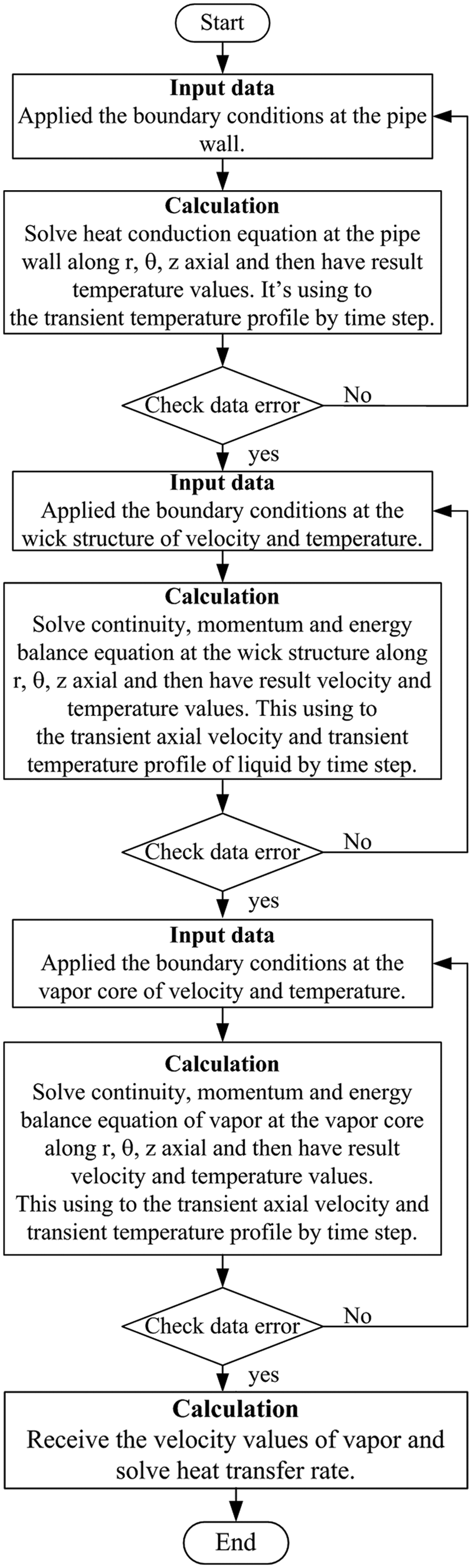Determining the heat transfer rate was found by using this equation $Q = \overset{\cdot}{m} c_{p} (T_{out} - T_{in})$ .^14,15 The experimental setup with the test rig is shown in Figure 4, and photographic view of the experimental setup is shown in Figure 5.

Figure 3.

Schematic diagram of numerical procedure.

Figure 4.

Schematic diagram of the experimental setup.

Figure 5.

Photographic view of the experimental setup.

Results and discussion

According to equation (1), the computation domain in the $r, θ, and z$ coordinates of the three-dimensional model is represented in Figures 6 –8 and is compared with the experimental data. The working fluids were water, ethanol, and r134a, respectively. The transient condition temperature profiles were the average values for the evaporator section, adiabatic section, and condenser sections and were plotted as functions of time. It was found that the transient condition temperature profiles in the evaporator section increased from the initial temperature in the pipe wall to the temperature that was input to the evaporator section. Since the material of the pipe wall was copper, thermal conduction was then induced from the outer wall to the inner wall. The adiabatic section experienced no effect from the ambient heat, but heat was induced by thermal conduction from the evaporator section, and thus, the temperature of the adiabatic section increased until it reached a steady state. However, the transient temperature profiles in the condenser section decreased because the temperature at the outer wall was less than the initial temperature of the condenser section. As shown in Figures 6 –8, the times required to reach the steady state from the model were about 1500, 1400, and 1200 s, respectively. When the heat input at the evaporator section increased, the time required to reach the steady state increased because the temperature was dependent on the time.

Figure 6.

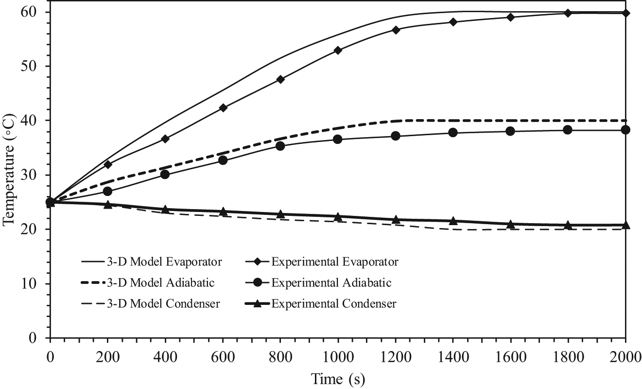
Transient temperature profiles in the pipe wall where working fluid is water.

Figure 7.

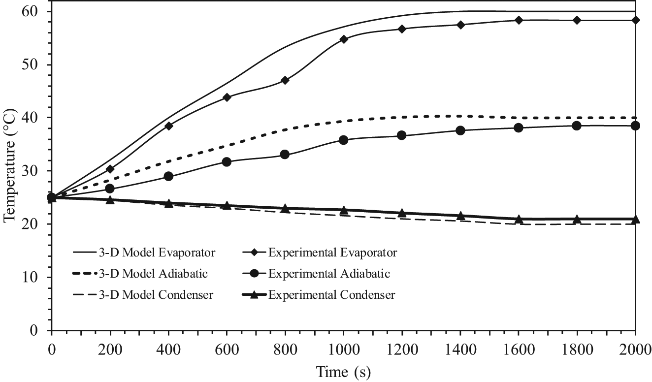
Transient temperature profiles in the pipe wall where working fluid is ethanol.

Figure 8.

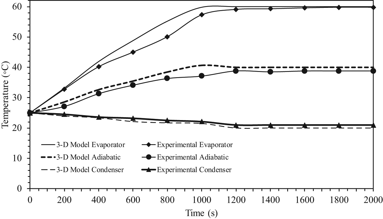
Transient temperature profiles in the pipe wall where working fluid is r134a.

The symbols correspond to the experimental average values of the temperatures at each section, and the times required to reach the steady state from experiment were about 1800, 1600, and 1500 s, respectively. As can be seen from these figures, the comparisons of the response curves between the results of the experimental and the three-dimensional model were excellent for all three sections. It was also observed that the time required to reach the steady state of experiment was longer than the mathematical model because we had assumed no loss of heat energy externally during transfer. As seen from all of the figures, the time required to reach the steady state between the three-dimensional model and the experiment results was different, and the differences were 4.5%, 3.75%, and 3%, respectively. The time required to reach the steady state is an important parameter for the start-up of a heat pipe. The time required to reach the steady state is defined as the time required to reach 95% of the corresponding steady-state values. This has been calculated from the theoretical results and is evaluated from experiments as well.¹⁶ The two values are in good agreement. It should, however, be mentioned that heat recovered at the condenser section is always lower than the heat added to the evaporator section due to uncontrolled heat losses from the experimental setup.

The velocity profiles of the liquid phase in the wick structure were compared with the model for each working fluid, as shown in Figure 9. It was found that the evaporator section exhibited a greater velocity than the adiabatic and condenser sections because the evaporator section experienced the heat source directly, but the velocity of the liquid in the condenser section was influenced only by the porosity of the wick structure. The velocity values were negative. This means that the liquid flow was along the inverse z direction. The times required to reach the steady state of the water, ethanol, and r134a were about 3200, 3000, and 2800 s, respectively. As a result, the three-dimensional transient axial velocity profile of the vapor phase inside the vapor core of the evaporator section at 60 °C is shown in Figure 10. A comparison among the three working fluids reveals that as the time increased, the velocity of the vapor phase increased, especially in the adiabatic section. The times required to reach the steady state of the vapor and liquid phases were equivalent. However, the velocity value of the vapor phase is positive because the vapor flow was along the z direction.

Figure 9.

Transient axial velocity profile of the liquid phase in the wick structure.

Figure 10.

Transient axial velocity profile of the vapor phase in the vapor core.

Figure 11 shows the comparisons of the simulation model and experimental heat transfer rate profiles in the transient condition of the heat pipe. These figures identify the time required to reach steady state as 3045 s for the simulated model and 3360 s from experimental data where the working fluid is water. The times using ethanol for simulation and experiment were 2940 and 3100 s, respectively. And it is seen that the times required to reach steady state were 2520 and 2900 s from simulation and experiment using r134a. Therefore, the time required to reach steady state depends on the working fluid used. It can be seen that the heat transfer rate profiles between the simulation and experiment were very similar, with the differences being 3.3%, 4.6%, and 2.0% for the working fluids of water, ethanol, and r134a, respectively.

Figure 11.

Comparison of transient heat transfer rate profiles between the model and experimental data.

Figure 12 shows the results of the wall temperature distributions from the numerical simulation model, which was carried out using the experimental parameters, compared with the analytical data obtained by Sonan et al. Their model was a transient three-dimensional thermal model of a flat heat pipe wall.¹⁷ However, this study involved a three-dimensional model in the transient condition of a cylindrical heat pipe wall, so it has to become normalized by the time required to reach the steady state. It appears that the trend is one of similar temperatures. The temperatures quickly increased during the first time period. During the second time period, the temperature slowly increased and then rose to a steady state. The increase in temperature up to the steady state of the flat-shaped heat pipe wall was more dramatic than that of the cylindrical shape because there was less cross-sectional area to receive the immediate heat. Thus, the heat transfer rose quickly to the steady state.

Figure 12.

Comparison of temperature profiles between this study and those of Sonan et al.¹⁷

Conclusion

The transient three-dimensional simulations of the outer wall, wick structure, and vapor core of a heat pipe have been successfully conducted using the finite element method. The temperatures from the developed three-dimensional model of the outer wall were in good agreement with the analytical data suggested by Sonan et al. The working fluid r134a required the shortest time to reach the steady state. The calculation time was approximately 8 h using a desktop computer with a CPU operating frequency of 3.90 GHz. However, the present simulation codes are still under development for overall heat pipe simulation, and they should become a strong tool to predict overall heat pipe operation in the future.

Footnotes

Appendix 1

Academic Editor: Mario L Ferrari

Declaration of conflicting interests

The authors declare that there is no conflict of interest.

Funding

The authors gratefully acknowledge the Royal Golden Jubilee PhD Program (grant no. PHD/0014/2554) under the Thailand Research Fund (TRF) for funding this research.

References

Marcus

. Theory and design of variable conductance heat pipes. NASA Technical Reports Server, NASA-CR-2018, 1 April 1972, p. 248. Washington, DC: NASA.

Vlassov

Riehl

. Mathematical model of a loop heat pipe with cylindrical evaporator and integrated reservoir. Appl Therm Eng 2008; 28(8–9): 942–954.

Nemec

Čaja

Malcho

. Mathematical model for heat transfer limitations of heat pipe. Math Comput Model 2013; 57(1–2): 126–136.

Tournier

El-Genk

. A heat pipe transient analysis model. Int J Heat Mass Tran 1994; 37(5): 753–762.

Jang

Faghri

Chang

. Analysis of the one-dimensional transient compressible vapor flow in heat pipes. Int J Heat Mass Tran 1991; 34(8): 2029–2037.

Faghri

. Heat pipe science and technology. Washington, DC: Global Digital Press, 1995.

Suman

DasGupta

. Transient modeling of micro-grooved heat pipe. Int J Heat Mass Tran 2005; 48(8): 1633–1646.

Ranjan

Murthy

Garimella

. A numerical model for transport in flat heat pipes considering wick microstructure effects. Int J Heat Mass Tran 2011; 54(1–3): 153–168.

Choudhary

Karki

Patankar

. Mathematical modeling of heat transfer, condensation, and capillary flow in porous insulation on a cold pipe. Int J Heat Mass Tran 2004; 47(26): 5629–5638.

10.

Thuchayapong

Nakano

Sakulchangsatjatai

. Effect of capillary pressure on performance of a heat pipe: numerical approach with FEM. Appl Therm Eng 2012; 32: 93–99.

11.

Vafai

Wang

. Analysis of flow and heat transfer characteristics of an asymmetrical flat plate heat pipe. Int J Heat Mass Tran 1992; 35(9): 2087–2099.

12.

Schmalhofer

Faghri

. A study of circumferentially-heated and block-heated heat pipes—II. Three-dimensional numerical modeling as a conjugate problem. Int J Heat Mass Tran 1993; 36(1): 213–226.

13.

Chen

M-M

Faghri

. An analysis of the vapor flow and the heat conduction through the liquid-wick and pipe wall in a heat pipe with single or multiple heat sources. Int J Heat Mass Tran 1990; 33(9): 1945–1955.

14.

Sriudom

Rittidech

Chompookham

. The helical oscillating heat pipe: flow pattern behaviour study. Adv Mech Eng, http://www.hindawi.com/journals/ame/aa/194374/

15.

Jengsooksawat

Rittidech

Booddachan

. Loop thermosyphon with vapour chamber: a thermodynamic study. Adv Mech Eng 2014; 2014: 1–8.

16.

Mistry

Thakkar

. Experimental validation of a two-dimensional model of the transient and steady-state characteristics of a wicked heat pipe. Exp Heat Tran 2010; 23(4): 333–348.

17.

Sonan

Harmand

Pellé

. Transient thermal and hydrodynamic model of flat heat pipe for the cooling of electronics components. Int J Heat Mass Tran 2008; 51(25–26): 6006–6017.

Three-dimensional transient mathematical model to predict the heat transfer rate of a heat pipe

Abstract

Keywords

Introduction

Modeling approach

Heat conduction of the pipe wall

Fluid flow of vapor phase in the vapor core

Fluid flow of liquid phase in the wick structure

Heat transfer rate of a heat pipe

Boundary conditions

Numerical scheme and experimental setup

Results and discussion

Conclusion

Footnotes

Appendix 1

Declaration of conflicting interests

Funding

References