
Abstract
Aiming at the problems of laser Simultaneous Localization and Mapping (SLAM), such as drift, low localization accuracy and map ghosting, which are prone to occur during localization and map construction in different structured environments, a tightly-coupled SLAM method of lidar and Inertial Measurement Unit (IMU) is proposed. Specifically, the initial position information provided by the IMU for the lidar is used to construct the joint error function of the IMU and the lidar, so as to achieve iterative position optimization. Following, the variety of the environmental structural information is determined, using a degradation detection method, based on the perturbation model, thus the selection of different methods for position estimation in different featured environments is achieved. Finally, when adequate number of structured features is obvious, the algorithm based online and surface feature matching, as proposed in LOAM, is used for motion estimation between neighboring frames. In the case of structural information lacking, the Iterative Closest Point (ICP) algorithm, containing distribution shape constraints, is introduced, to increase the constraints on the effective observation data, improving the stability and accuracy of the system, under the premise of ensuring that the system can run in real time. The results of extensive testing and validation in different scenarios, using open-source datasets, show that the proposed algorithm has higher accuracy and environmental adaptability, compared to other commonly used algorithms. In addition, real-vehicle tests, based on an autonomous self-driving car test platform, further demonstrate that the proposed method can be adapted to long-time drive and large-scale working environments, while it can operate steadily in real time.
Introduction
Simultaneous localization and mapping (SLAM), where external sensors (including lidar, IMU, GPS and other sensors) are used to collect environmental information, while then the collected information is processed and matched, finally realizing mapping and localization, is a hot spot of research in the fields of mobile robots and unmanned vehicles.1–6 Depending on the sensors used, SLAM can be classified into two types: visual SLAM and laser SLAM. Compared to visual sensors, lidar has high ranging accuracy, is not easily affected by external disturbances, such as light and change of viewing angle, it has the features of intuitive and convenient map construction, high robustness for map building and is widely used in various indoor and outdoor scenes.7–12 lidar is distinguished into 2D lidar and 3D lidar, according to the number of lasers. 2D laser SLAM technology is mature and widely used in service robots and industrial sites, but it cannot be applied to all-terrain environments, as it cannot achieve localization and map construction when there are undulations or ramps. 3D lidar achieves an accurate representation of the environment structure by emitting multiple laser beams to measure the geometric information of objects in its surroundings and acquiring point cloud data containing precise distance and angle information.13–18
Currently, a mature 3D laser SLAM framework consists of four core modules: front-end scanning and matching, back-end optimization, loop-back detection and map construction. Based on the point cloud data measured by lidar, the front-end performs inter-frame alignment through scanning matching, closed-loop detection, to obtain the relationship of point cloud data between different frames, continuous updating of position estimation and storage of corresponding map information. A system for real-time high precision 3D mapping of the surrounding environment is proposed in Li et al., 19 which enables quick and convenient operation to obtain high precision data. The positioning accuracy in urban environments can reach 0.06%. Literature 20 proposed a continuous time lidar inertial odometry (CT-LIO) system, which is more efficient than commonly used nonlinear solvers. The back end obtains the maximum likelihood estimation of the constructed map, along with the robot position, by maintaining and optimizing the robot position and observation constraints obtained from the front-end.21–23 As the mass production and popularity of lidar increases, 3D lidar has started to move toward low-cost, low-power and high-reliability applications, while 3D lidar-based SLAM algorithms are being rapidly developed. LOAM 24 (Lidar Odometry And Mapping) is the most representative 3D laser SLAM algorithm, different from traditional algorithms such as NDT 25 and ICP, 26 which proposes the concept of feature points and improves the efficiency of the alignment by replacing the alignment between the whole point cloud with the alignment between the corner points and the plane points. By running map building and positioning separately at different frequencies, it achieves fast speed, high accuracy and good robustness. However, the lack of back-end optimization leads to a more serious drift problem, arising from large environment map building. SHAN introduced a point cloud segmentation and loop-back detection module, to solve the problem of degradation of solution accuracy, caused by insufficient stability of point features in LOAM, proposing LEGO_LOAM, 27 which achieves a similar or even better accuracy while requiring less computational resources. An even more enhanced approach is the open-source livox_loam, 28 from the University of Hong Kong, which employs a more stringent strategy for feature point extraction and adds filtering of outlier and dynamic points, as well as loop-back detection. M_LOAM 29 improves the perception range of the robot, by combining inputs from multiple lidars, constructing a global map and combining enough observations to optimize the position estimation and try to reduce the measurement and estimation uncertainty. However, these SLAM algorithms, which only use lidar to obtain observations, are prone to the problem of positioning drift, when faced with excessive speed or steep corners.
A single sensor cannot complete the global map construction in all scenes, while multi-sensor fusion can solve the limitations of a single sensor and provide more accurate, efficient and adaptable SLAM results. The fusion of lidar and Inertial Measurement Unit (IMU) can overcome the problems of low vertical resolution of lidar, low update rate and motion-induced distortion, during laser SLAM. The LOAM approach relies on the IMU to solve the orientation, as an aid, using the IMU as source of a priori information for the whole system. However, it uses a loosely coupled lidar and IMU, while it cannot use IMU measurements for further optimization. LIO_mapping 30 proposed for the first time a tightly coupled lidar_IMU fusion method. By jointly optimizing the IMU and lidar measurements, there is no significant drift short-term, even with lidar degradation. On the other hand, the tightly coupled algorithm has high complexity and poor real-time performance. SHAN presented LIO_SAM, based on their proposed LEGO_LOAM, using IMU and lidar tight coupling. 31 The algorithm applies a factor graph framework, fusing IMU pre-integration factors, odometer factors, GPS factors and closed-loop detection factors, to obtain better real-time performance and accuracy in building the graph and positioning. Fast_LIO 32 reduces the computational complexity, from the measurement dimension to the state dimension, by an equivalent Kalman formula, while the computational efficiency is significantly improved. Based on Fast_LIO, the original authors also proposed the Fast_LIO2 33 lidar inertial odometer framework, which directly aligns the raw point cloud to the map, while at the same time introduces the ikd_tree data structure, to maintain the map, supporting incremental updating and dynamic balancing, which further improves the computational efficiency, but has poor robustness in the face of feature deficient environments. In recent years, the Point_LIO 34 laser inertial odometry method has been proposed, which uses a single point cloud as the data processing unit, updates the state of each point, and has extremely high odometer output frequency and bandwidth.
It is evident that, in the current research of 3D laser SLAM algorithms, it is difficult to complete global map construction and real-time localization in all scenarios, using only a single sensor, and it is especially easy for localization drift to occur in scenarios with degraded features. In addition, laser inertial tight coupling in featureless environments can still lead to low positioning accuracy, drift, etc., due to the reduction of valid observations and lack of constraints. In order to solve the above problems, this paper adopts a 3D lidar and IMU tightly coupled map building method, which fuses the ICP algorithm, introducing distribution shape constraints, with the feature-based point cloud alignment algorithm, based on the richness of structured information, as determined according to the difference of feature information in the actual environment. On the one hand, the use of feature-based matching algorithms in structured information-rich scenarios can reduce a large number of point cloud alignments and improve the efficiency of point cloud processing, under the premise of ensuring matching accuracy. On the other hand, ICP algorithms that incorporate distribution shape constraints are used in environmental degradation scenarios, that is, scenarios with less structured information, to improve the effective observations and increase the constraints. Considering the distribution shape and IMU error into the cost function. The main contributions of our work can be summarized as follows:
(1) A tightly coupled laser radar inertial odometry framework has been established, which is suitable for multi-sensor fusion and global optimization.
By tightly coupling lidar and IMU, the positioning accuracy in different environments is improved. In addition, additional sensor measurements can easily be incorporated into this framework as new factors.
(2) A hybrid scanning matching algorithm based on scene judgment is proposed. According to the different feature information in the actual environment, the richness of structured information is used as the basis for judgment and the ICP algorithm that introduces distribution shape constraints is fused with the feature-based point cloud alignment algorithm, which avoids to a certain extent the problem of reduced matching accuracy due to the environment degradation problem.
(3) Construct the joint error function of IMU and Lidar to minimize the total error of SLAM system. This method not only improves the convergence speed of point cloud registration, but also further corrects IMU errors in the SLAM process, achieving collaborative iterative optimization of position and attitude.
Compared to the Fast_LIO2, the advantages of the FI_LoMapping algorithm proposed in this paper are reflected in scene adaptability, matching strategy, and error constraints. On the one hand, the point cloud registration of Fast_LIO2 only considers the spatial distance of point clouds without additional constraints. The improved ICP algorithm of FI_LoMapping incorporates the distribution shape difference and IMU error into the cost function, adds mean and covariance constraints of Gaussian distribution and even if the distance between corresponding points is close, the mismatch of distributions will trigger error penalties, reducing incorrect matches. On the other hand, Fast_LIO2 reduces computational complexity through iterative Kalman filtering, focusing solely on state dimension optimization. FI_LoMapping constructs an IMU-Lidar joint error function, iteratively optimizes pose and IMU errors during the SLAM process and simultaneously fuses three types of factors: IMU pre-integration, laser odometry, and loop detection through a factor graph, avoiding the local optimum problem of a single sensor. In addition, compared to another LIO_SAM algorithm, the FI_LoMapping algorithm addresses the limitations of LIO_SAM, which lacks scene differentiation and has a single matching strategy. On the one hand, LIO_SAM is based on LEGO_LOAM’s ground optimization and feature extraction, and only adopts a fixed strategy of line-surface feature matching, resulting in unstable feature extraction in weak feature environments. FI_LoMapping, also built on the LEGO_LOAM framework, incorporates a scene determination module, integrating an adaptive tight-coupling framework of feature matching and distributed constraint ICP. On the other hand, LIO_SAM’s matching relies entirely on corner/plane point line-surface features, without an ICP registration step, leading to poor registration results when features are insufficient. FI_LoMapping combines feature matching with an improved ICP. For ICP in degraded scenes, it reduces computational load through voxel grid downsampling, enhancing constraint strength while maintaining real-time performance.
The remainder of the paper is organized as follows: System framework design is described in Section 2. Algorithm design is presented in Section 3. Simulation analysis is shown in Section 4 with thorough analysis. Vehicle testing is narrated in Section 5. A final conclusion is drawn in Section 6. The meanings of all symbols in the paper can be found in Appendix 1.
System framework design
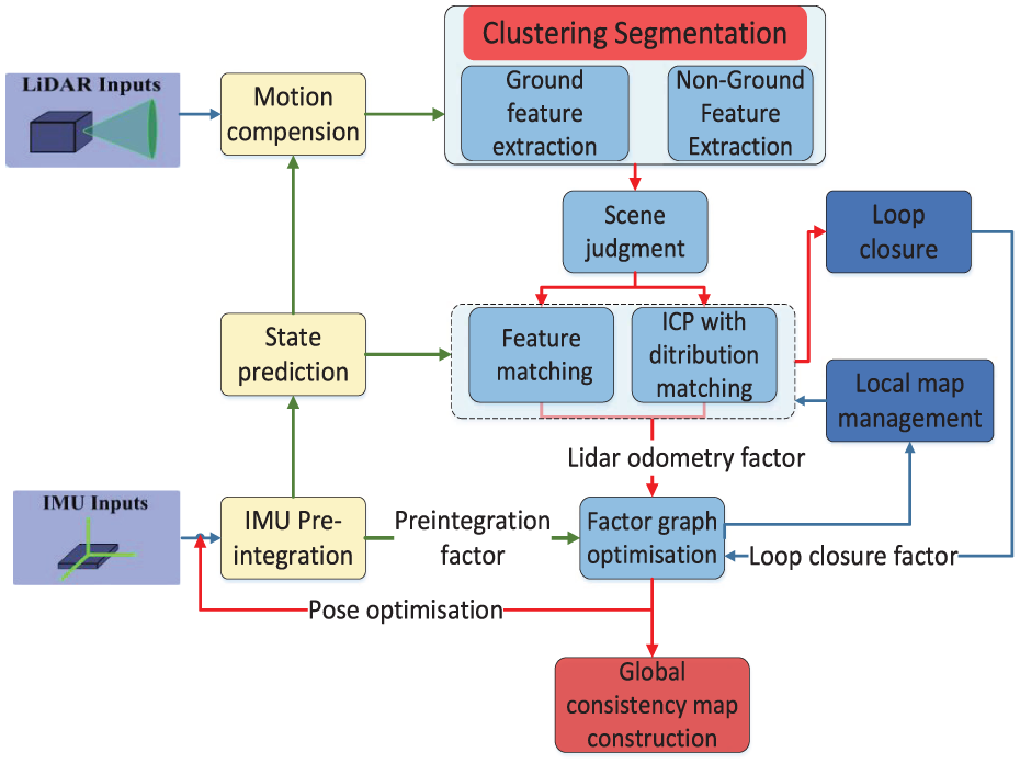
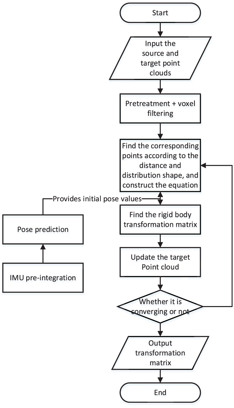
In this paper, a SLAM algorithm, based on LEGO_LOAM, is proposed, for tightly coupled lidar and IMU operating in different structured environments. The system framework is shown in Figure 1. A perturbation model-based approach is used to determine whether the environmental features are degraded or not, while a feature-based matching algorithm is used in non-degraded environments, to improve the efficiency of point cloud processing, thus ensuring the matching accuracy. The ICP algorithm that introduces distribution shape constraints is used in degraded environments, to increase the effective observation data constraints. The system framework consists of the following modules:
(1) IMU pre-integration. Integrate the IMU data within the corresponding lidar time frame interval, according to the IMU motion equation, to obtain the laser point cloud position at the corresponding time instance.
(2) Motion compensation. The relative positional attitude, as obtained from IMU pre-integration, is used to define each point cloud with relation to a frame projected to the initial instance of the time frame.
Feature extraction. The extraction of surface and edge features of ground and non-ground areas is performed on the basis of point cloud clustering segmentation.
(3) Scene determination. Based on the perturbation model and the extracted feature points, the structure of the current environment is determined, the point cloud matching algorithms, based on the feature and the ICP with the introduction of distribution shape constraints, are selected, respectively.
(4) Local map construction and optimization. Joint feature extraction points, IMU pre-integration factors and back-end position correction are used to construct local maps.
(5) Closed-loop detection and factor map optimization. Match the new local maps with the stored local maps at certain intervals of time or distance. By detecting the loop, combining the loop factor, lidar odometer factor, and IMU pre-integration factor, the front-end matching results are further optimized to obtain the final estimated position.
3D Lidar SLAM algorithm flow.
Algorithm design
Point cloud pre-processing
The point cloud captured by 3D lidar is used as input to the ground segmentation module, where it is segmented using Patchwork 35 and the laser odometry framework. The method projects the original point cloud and the ground point cloud onto the two images and performs in-plane and edge feature extraction, for both the ground and non-ground point clouds.
Due to the uneven distribution of points naturally generated by lidar, feature points can be extracted from the lidar point cloud. We select feature points that are on sharp edges and planar surface patches. Let
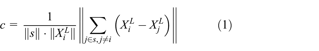
Where,
Where,
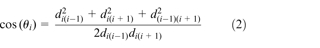
In practical environments, the cosine value of the angle between scanning points on a plane is theoretically −1. Due to the presence of noise, the cosine value interval of the plane points is set to [−1, −0.984], the angle is within
Select four planar points (a total of 24 scanning points) as planar points for each subgraph with cosine values closest to −1.
For cosine values close to −1, select four candidate plane points for each subgraph (a total of 24 scanning points).
The cosine value closest to 0, select two corner points for each subgraph (a total of 12 scanning points).
For cosine values close to 0, select two candidate corner points for each subgraph (a total of 12 scanning points).
IMU attitude estimation
Compared with force sensors for measuring force and torque,36,37 inertial IMU measures the motion parameters of the carrier itself, while its internal accelerometer and gyroscope measure specific force and angular velocity, respectively. Through integration calculation, the carrier’s three-axis attitude, velocity, and position information in space can be finally output.
38
The raw measurement value of IMU contains three parts: real motion information, deviation, and noise. Directly using this raw measurement value may lead to the accumulation of subsequent pre integration errors. Therefore, the following formula can be used to obtain preliminary estimates of the true angular velocity
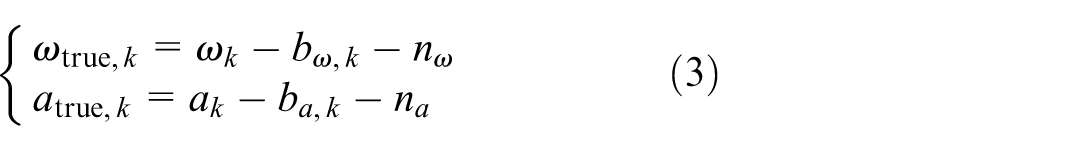
Where,

Where,

To describe the difference between the IMU predicted attitude

Based on the above attitude angle increment

Where,

Where,
Detection of degradation of environmental features
Inspired by the improved results presented in literature 39 regarding the position estimations under environmental degradation, this paper uses a perturbation model-based approach to determine the degree of degradation of environmental features. The lidar-based position estimation problem, which is ultimately transformed into a non-linear least squares solution problem:
Where,

Where,
Where,
Combining equations (11) and (12), we can calculate

The degradation characterization factor
When the perturbation of

To reduce computational resource consumption,
The distance between matrices can be measured using the Frobenius norm, where the difference between

Where,

Where, The eigenvectors corresponding to the six eigenvalues mentioned above are
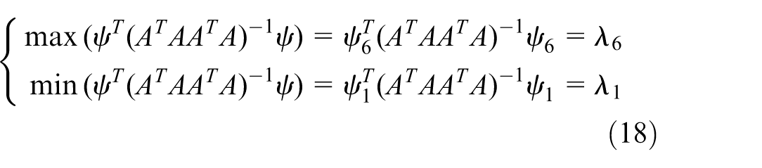
It can be seen that when disturbance equations are applied to the original system of equations, the maximum and minimum changes in the optimal solution can be represented by the maximum value
Lidar point cloud motion compensation
In order to solve the problem of point cloud distortion, caused by carrier motion, IMU pre-integration is used for state estimation. The state of the IMU is estimated based on the data between frames of the point cloud, while a pre-integration operation is performed on the IMU measurements.


Where,


The deviation of the angle


Based on the IMU position before and after the five time instances, the position of the five laser point clouds is obtained and quadratic curve fitting is performed, to obtain the curve fitting equation of the position of the point cloud for each frame. Finally the current frame of the point cloud is corrected according to the curve fitting equation.
Hybrid scanning matching algorithm
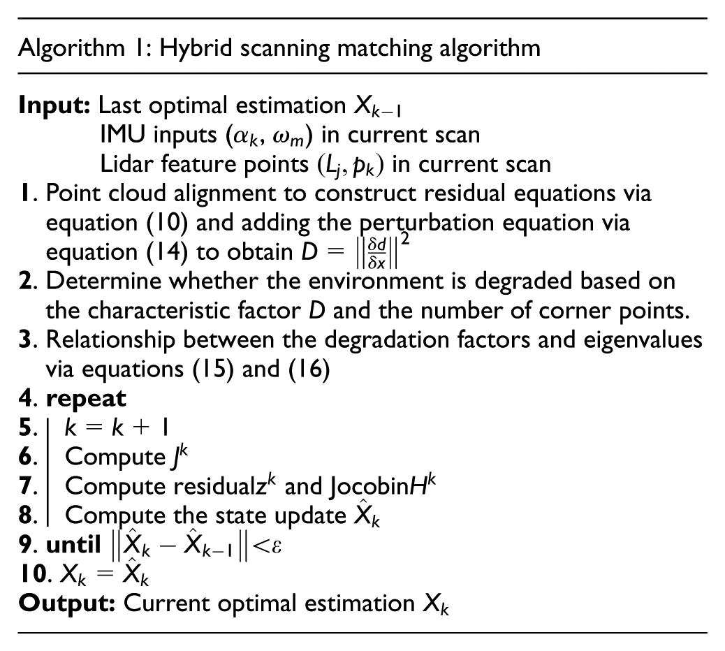
In structured information-rich scenarios, due to the large number of alignment points, the point-to-point based ICP matching algorithm is computationally inefficient. In scenarios with less structured information, it is difficult for feature-based matching algorithms to extract stable and reliable features, making those based on line and surface features perform less well. Therefore, a hybrid scanning matching algorithm is proposed in this paper. Based on a perturbation model-based approach, it is determined whether the environmental features are degraded. A point-to-line and surface-based feature matching algorithm is used in scenarios with rich environmental features. When the environmental features are degraded and sufficient constraint information cannot be extracted, the ICP scanning matching mode, which introduces distributed shape constraints, is activated. The pseudo-code for the hybrid scanning matching algorithm is shown as follows:
Line and surface feature matching
After the pre-processing session, the point cloud of a frame is divided into edge and planar points, which are difficult to handle using each lidar frame for computation. Therefore, the concept of key frames is introduced, where a new key frame is added, when the change in the robot’s position, compared to the previous state, exceeds a user-defined threshold (in this study, this value is 1 m and
(1) Sub-keyframe map: The sliding window method is used to create a point cloud, containing a fixed number of lidar scans. Instead of optimizing the transition between two consecutive lidar scans, this paper extracts the nearest
(2) Joint optimization function: according to the LOAM algorithm, it is known that the error function, based on points to lines and surfaces, can be expressed as follows:
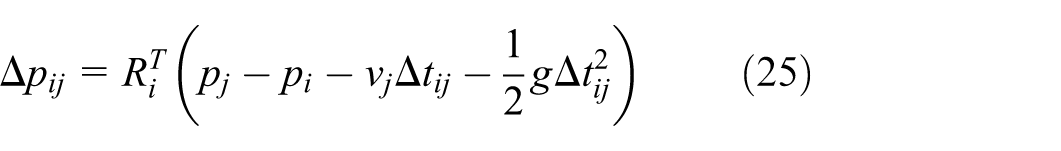
By using equations (23)–(25), the error function of the IMU can be constructed as follows:

Next, the joint error function of IMU and lidar, under feature-based matching, is constructed as:

ICP-based with distribution matching algorithm
The standard ICP matching algorithm finds a matching counterpart for each point in the point set, using the nearest Euclidean distance criterium, which is highly inefficient.
22
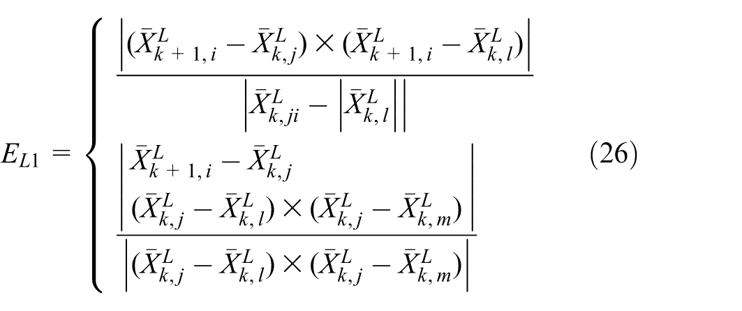
There are irrationality in this assumption, and a certain number of incorrectly corresponding points are generated during the matching process. Based on this, voxel grid maps are used in a way to reduce the number of points used for point cloud alignment, without limiting the matching accuracy as a result. The cost function used includes not only the distances between the points of the same name, the IMU error function, but also the differences between the shapes of the distributions. In this case, even though the distance between points of the same name is small, the same mismatch in the shape of the distributions leads to a large cost function and thus non-convergence. The flowchart for improving the ICP algorithm is shown in Figure 2. Since ICP is a distance minimization algorithm, the scatter with symmetry of two Gaussian distributions
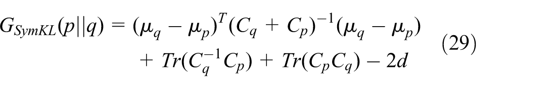
Where,
ICP-based distribution matching algorithm flowchart.
To further address the effects of outliers, the ICP error


Where,

In above equation (32),
Loop closure and back-end optimization
Loop closure: Loop closure is an important part of SLAM to identify robots revisiting known locations and correct navigation errors. The lack of loop-back detection will lead to problems such as accumulation of positioning bias, inaccurate maps and reduced navigation efficiency. In long-range or wide-range operations, loop closure is critical to ensuring the accuracy and performance of SLAM systems. In order to improve the efficiency and accuracy of Loop closure, (1) Set the minimum time difference: As the carrier advances, key frames are continuously generated, while it is undoubtedly too time-consuming to detect all past frames, so the concept of interval key frames is introduced, in order to loop back in the key frames prior to the current frame-interval key frames. (2) Set a time delay for each test. (3) A loop-back is determined only when it is detected continuously, in order to avoid false matches.
Back-end optimization: the robot pose is further optimized by constructing a factor graph. The factor graph contains three types of factors, IMU pre -integration factors, lidar odometry factors and closed-loop factors, as well as the state of the robot at key time instances. As new state nodes are added to the factor graph, optimization is performed using a mapping of smoothing increments to Bayesian trees. By using the factor graph optimization method to construct the systematic error function of the three factors, the problem of local optimal solution caused by the construction of error equation by a single sensor and the problem of large difference between the calculated value and the actual value caused by the error of sensor data is avoided.
Simulation analysis
In this section, we present comprehensive experiments of the proposed hybrid scanning matching algorithm (defined as FI_LoMapping), including validation on public datasets. We compare FI_LoMapping with state-of-the-art and open-source methods, including LEGO_LOAM, Fast_LIO2, Point_LIO, LIO-SAM, all of which use their recommended parameters for simulation scenarios. The LEGO_LOAM and Fast-LIO2 algorithms construct the residual equation through feature point matching, and obtain the final positioning information by optimizing the residuals. The computing devices used were all Intel i9-9900KF, while the algorithms were executed under Linux and ROS, using only the CPU in the computation. The data collected in the KITTI public dataset from urban residential environments and the park dataset collected by TiXiaoShan mentioned in literature [16] were selected and defined as structured and unstructured scenarios, respectively.
Unlike industrial robotic arms that execute a high-precision, repeatable motion trajectory to complete a specific task in a known and structured environment,41,42 the trajectory output by SLAM systems needs to include the position and orientation of each moment in the future. The generation of trajectories is closely related to the vehicle’s driving environment, so trajectory error analysis needs to be carried out under different environmental and road conditions.
Point cloud map construction analysis
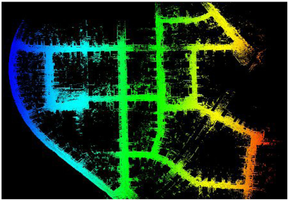
The data collected in two scenarios were fed into the LEGO_LOAM, Fast_LIO2, and FI_LoMapping algorithms, to obtain the respective point cloud maps (Figures 3 and 4). Figure 3(a)–(c) illustrate that, in the town scene, which is relatively rich in structured information, the effects of the point cloud maps constructed by the three algorithms are basically the same. In the park scene, as shown in Figure 4(a), the environment map constructed by FI_LoMapping has no obvious ghosting and drifting, whereas the Fast-LIO2 algorithm is shifted to some extent in the Z-axis (Figure 4(b) and (c)) and the LEGO_LOAM algorithm shows poor positioning accuracy during map building and drifts so badly that the map cannot be built.
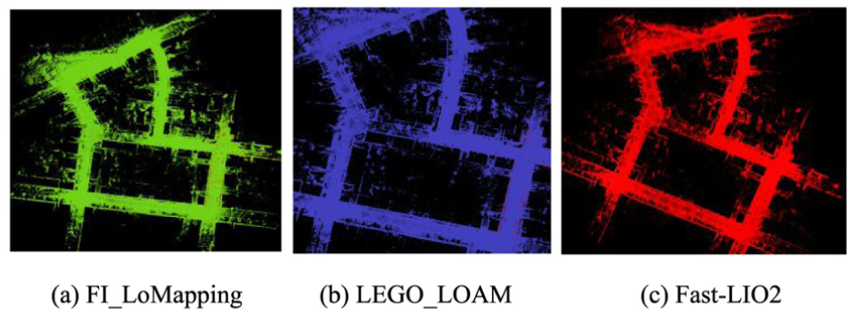
Cloud map of structured site attractions: (a) FI_LoMapping, (b) LEGO_LOAM and (c) Fast-LIO2.
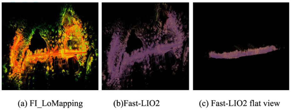
Cloud map of unstructured scene points: (a) FI_LoMapping, (b) Fast-LIO2 and (c) Fast-LIO2 flat view.
In order to further evaluate the map building performance of the five algorithms, the final output trajectories of the three algorithms in the two scenarios are compared as shown in Figure 5, where the dashed line indicates the trajectory true value. The overall trajectories, illustrated in Figure 5(a) and (b), demonstrate that the output trajectory of the FI_LoMapping algorithm is the closest to the real trajectory, while in cases of steep corners, the rotation angle, as estimated by the FI_LoMapping algorithm, is also closer to the real value, which indicates that the proposed FI_LoMapping algorithm produces a more accurate estimation of the trajectory, compared to other algorithms. In addition, it can be observed that LIO-SAM, as a lidar-inertial SLAM algorithm, is also based on feature extraction and factor graph optimization. On straight road segments without turns, its trajectory is similar to that of the FI_LoMapping algorithm and is relatively close to the true trajectory value. However, it tends to drift on curved road segments lacking features.
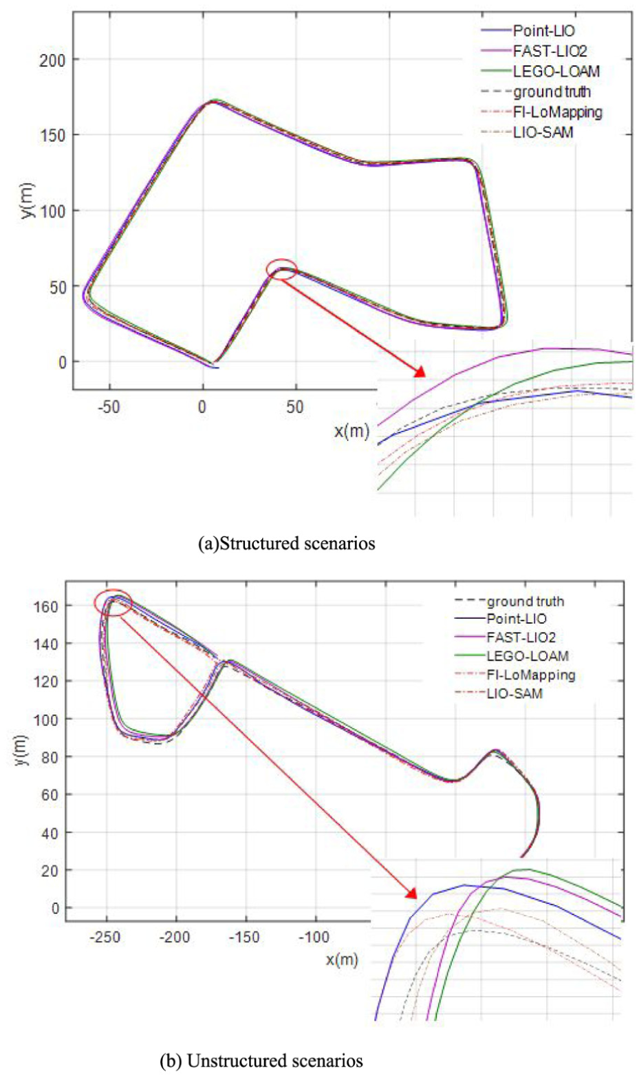
Algorithm output trajectory: (a) structured scenarios and (b) unstructured scenarios.
Comparative analysis of relative error
Each algorithm repeats the simulation 10 times, and records the maximum error, minimum error and average error in each simulation, while the average error is considered as the final positioning accuracy standard (Table 1).
Relative position error of algorithms in different scenarios.
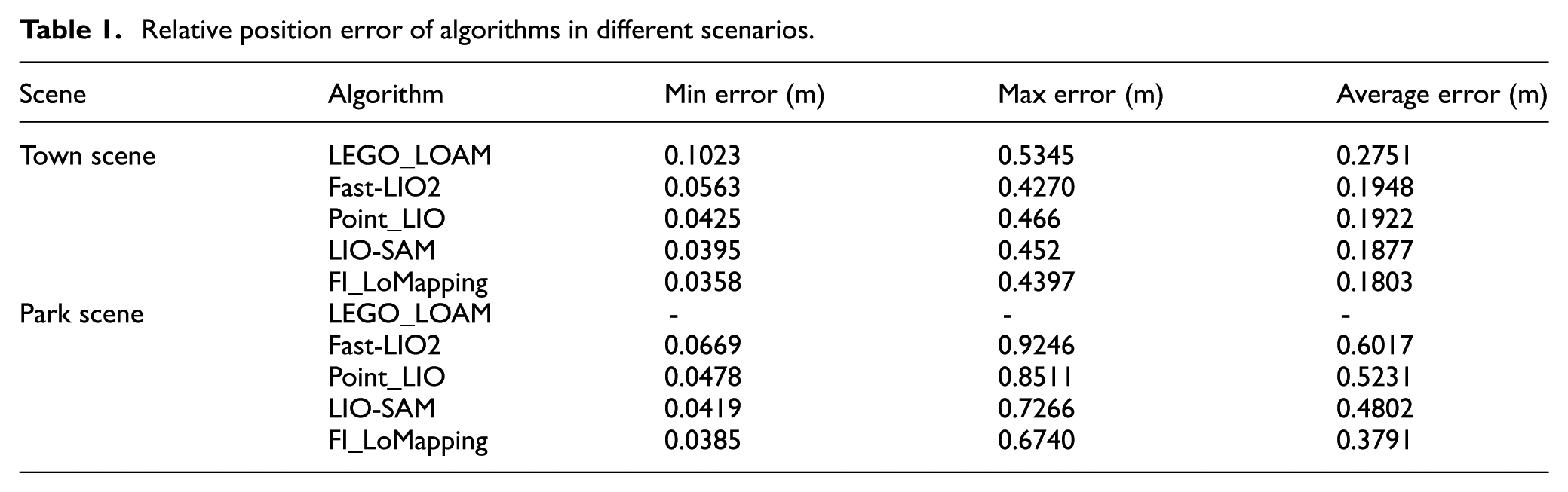
In the town scene, the FI_LoMapping algorithm outperforms the LEGO_LOAM, Fast_LIO2, Point_LIO, LIO-SAM algorithms by 34.5%, 7.4%, 6.2%, 3.9% respectively, in the structured and rich featured town scene. Due to the distinct features of buildings and roads in urban scenes, both LIO-SAM and the FI_LoMapping algorithm proposed in this paper exhibit good localization performance. In the park scene, where relatively little structured information available, the FI_LoMapping algorithm deviates a maximum of 0.6740 m and a minimum of 0.0385 m, which represents a 36.9%, 27.5%, 21.1% improvement over the Fast-LIO2, Point_LIO, LIO-SAM algorithm. In addition, LEGO_LOAM algorithm shows poor positioning accuracy during map building and drifts so badly that the map cannot be built.
Comparative analysis of cumulative error
On the basis of the alignment of the starting position of the five algorithms with the starting position of the real trajectory, the endpoint coordinates, estimated by the five algorithms, are compared with the endpoint coordinates given by the real trajectory, whereas the cumulative errors in the direction of the X, Y and Z coordinates axes are calculated respectively in Table 2.
Cumulative error of algorithms in different scenarios.
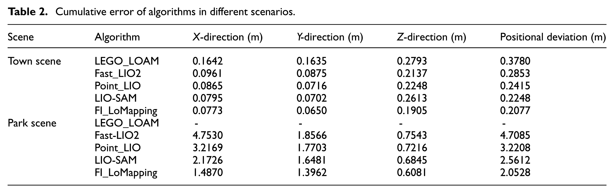
Evidently, Table 2 shows that, in the more structured town scenario, the relative error of the FI_LoMapping algorithm is reduced by 45.1%, 27.2%, 14%, 7.6% compared to the one produced by LEGO_LOAM, Fast_LIO2, Point_LIO and LIO-SAM algorithms, respectively. In the park scene, where there is a relative lack of structured information, the cumulative error of the FI_LoMapping algorithm is reduced by 56.4%, 36.3% and 19.8% respectively, compared to the Fast-LIO2, Point_LIO and LIO-SAM algorithm. As shown by the results, the FI_LoMapping algorithm produces smaller relative position error and cumulative error, compared to LEGO_LOAM, Fast-LIO2, Point_LIO and LIO-SAM algorithms, demonstrating better positioning accuracy and more obvious advantages in scenes with a lack of structured information. Compared to the current LIO-SAM algorithm, FI_LoMapping has undergone optimizations in scene adaptation, matching algorithm and loop closure optimization, addressing the limitations of LIO-SAM, such as lack of scene differentiation and a single matching strategy, thus resulting in smaller cumulative errors. In addition, the FI_LoMapping algorithm achieves scene degradation detection based on a perturbation model. It judges the environment through the number of features and a minimum feature value threshold, and adaptively switches matching strategies, enabling the algorithm to exhibit good localization performance in both town and park scenes.
Complex environment analysis
To analyze the impact of different steering angles and more challenging trajectory on positioning errors, a complex scene analysis was conducted. Select the 00 sequence dataset from KITTI for simulation, which includes multiple intersections and right angle turns and has the characteristics of small turning radius and high turning frequency, as shown in Figure 6. Dense buildings in the dataset can easily cause interference to sensors, leading to interruptions in observation data. This can effectively evaluate the pose estimation accuracy of SLAM algorithm in turning scenes.
Complex environment dataset.
Compared to the ground truth value of the trajectory, the positioning errors of the above five algorithms are shown in Figure 7 and the standard deviation and variance of positioning error are shown in Table 3.
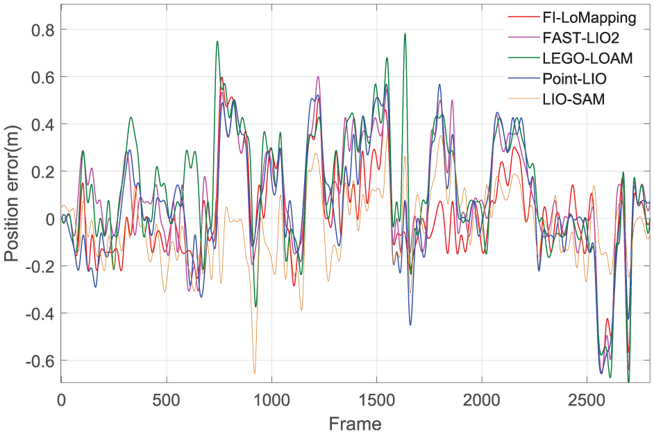
Positioning errors in complex environments.
Variance and standard deviation of positioning error.
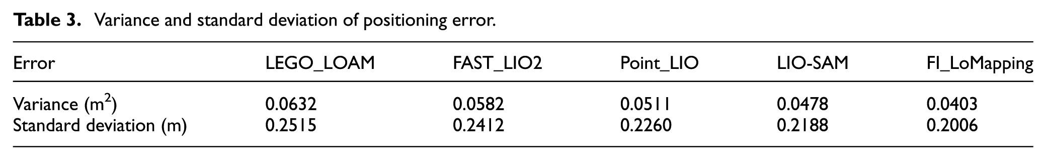
In Figure 7, it can be seen that in complex scenes with frequent turns, the maximum positioning error of the FI_LoMapping algorithm is 0.55 m, while the maximum positioning errors of the LEGO_LOAM, FAST_LIO2, Point_LIO, LIO-SAM algorithms are 0.78, 0.6, 0.66, 0.65 m respectively. In addition, in Table 3, the variance and standard deviation of the FI_LoMapping algorithm are 0.0403 m2 and 0.2006 m, which are 21.13% and 11.23% lower than those of the Point_LIO algorithm. Compared to LIO-SAM, the variance and standard deviation of FI_LoMapping have been reduced by 15.6% and 8.3%, respectively.
The trajectory curve of FI_LoMapping Algorithm is shown in Figure 8. It can be seen that the positioning error of FI_LoMapping is relatively small on straight road sections, but the error is large during the turning process. The main reason is that in straight road sections, the SLAM system can obtain more and more stable constraints to correct its position. When turning, these constraints become scarce and unstable in a short period of time, leading to error accumulation. In addition, during rapid steering of IMU, the accelerometer is affected by centrifugal force, resulting in more pronounced drift. However, compared to the other four algorithms, FI_LoMapping algorithm still has good reliability and higher positioning accuracy.
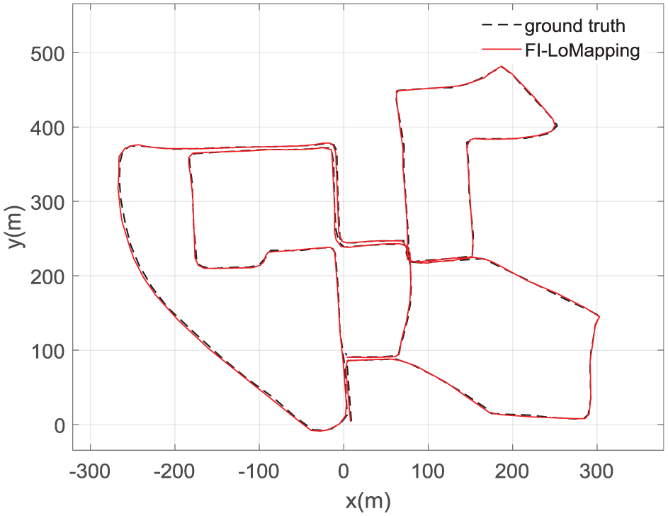
FI_LoMapping algorithm output trajectory.
Vehicle testing
A real vehicle testbed (Figure 9) is constructed, including a 16-line mechanical rotating lidar, IMU and a set of high-precision inertial combined navigation (INS/RTK; used only to provide true values for the SLAM system). The test vehicle is an autonomous vehicle that does not involve any human participants. The movement of the vehicle is controlled by a VRW-6700 computer with a quad core i5-7260U CPU.The experimental parameters and detailed configuration process can be found in Appendix 2.
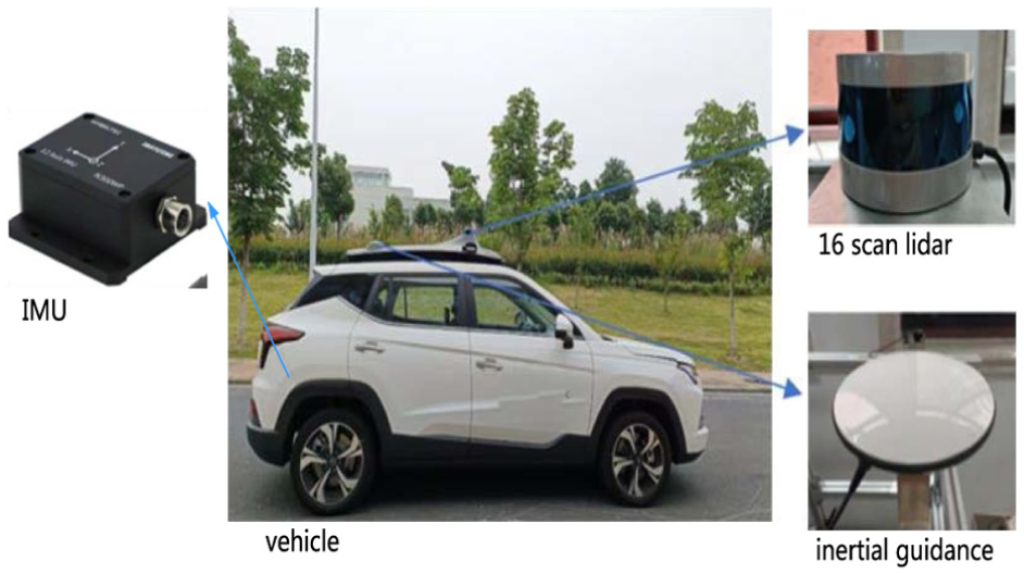
Real vehicle testbed.
Within the experimental environment, a building area with more structured information and a square lawn area with less structured information are selected (Figure 10) and denoted as area ① and area ②, respectively. The test road covers areas ① and ②, which consists of road I, road II and road III. The experimental path and its corresponding eigenvalue curve is shown in the lower part of Figure 10. It can be seen that when driving in the road I section that lacks features, the eigenvalue is lower than the threshold (the maximum eigenvalue) and in this area it is prone to reduced positioning accuracy or loss of positioning. In the boundary part of the two regions, namely road II, the eigenvalue fluctuates above and below the threshold value, while when driving in the section of road III with obvious features, the eigenvalue is higher than the set threshold value.
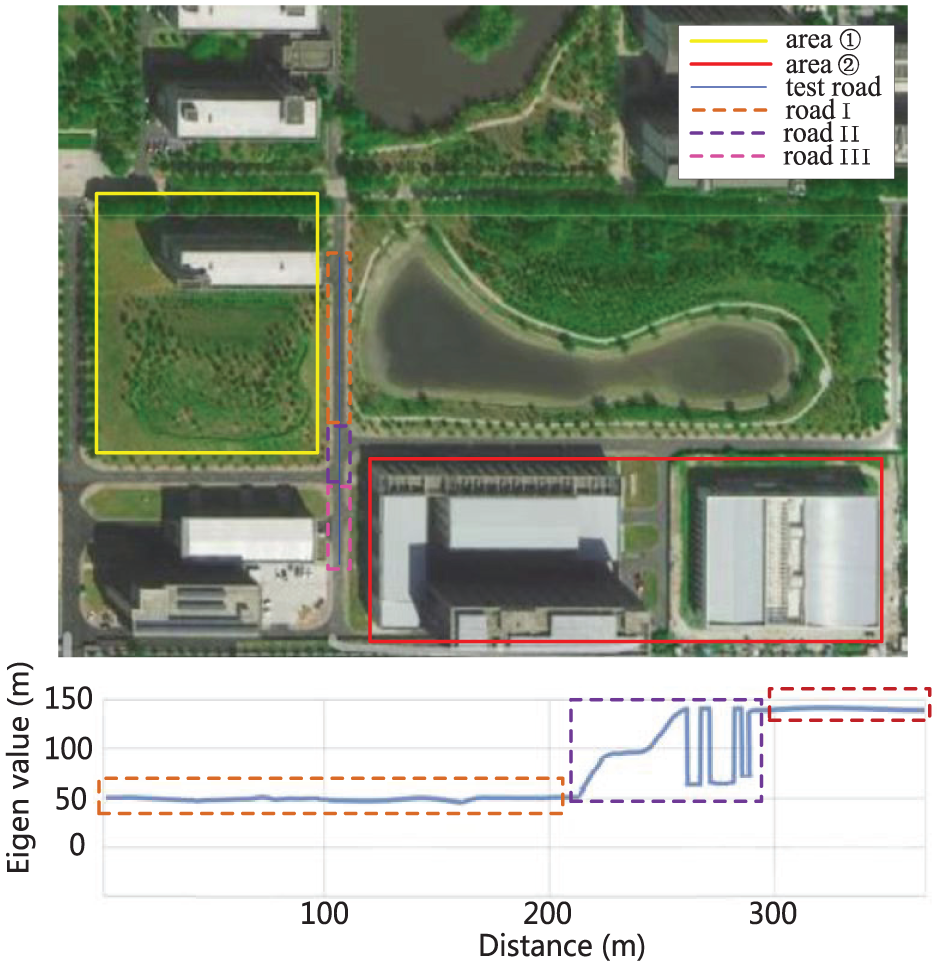
Experimental path and its corresponding eigenvalue curve.
Figures 11 and 12 show the output trajectories of each algorithm in region ① and region ②, respectively. It is evident that the cumulative error of each algorithm increases as the travel distance becomes longer, but compared to the other algorithms, the real-time estimation of the position trajectory by the FI_LoMapping algorithm is closer to the real value and produces the smallest cumulative error. In region ①, where there is a relative lack of features, the introduction of distribution shape constraints makes the advantages of the FI_LoMapping algorithm more obvious. For the straight road segments in Region ②, which are rich in structural features, both LIO-SAM and FI_LoMapping can effectively extract edge points and planar points, making their trajectories close to the true values. Compared to LIO-SAM algorithm, FI_LoMapping algorithm still has good reliability and higher positioning accuracy on curved road segments.
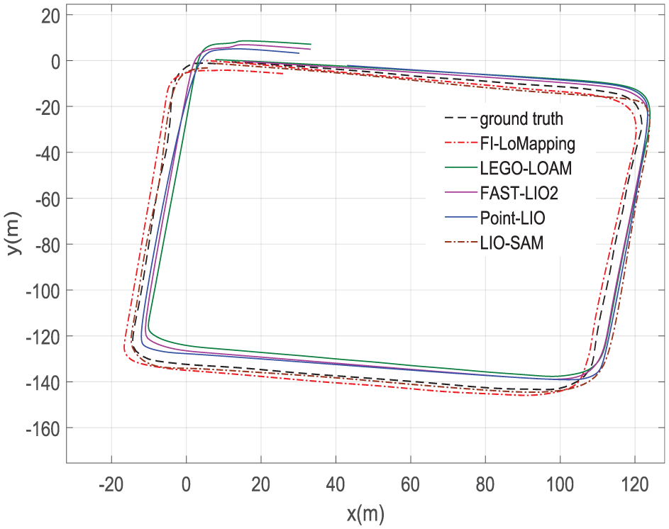
Comparison of algorithmic trajectories in region ①.
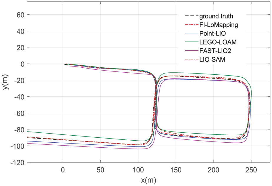
Comparison of algorithmic trajectories in region ②.
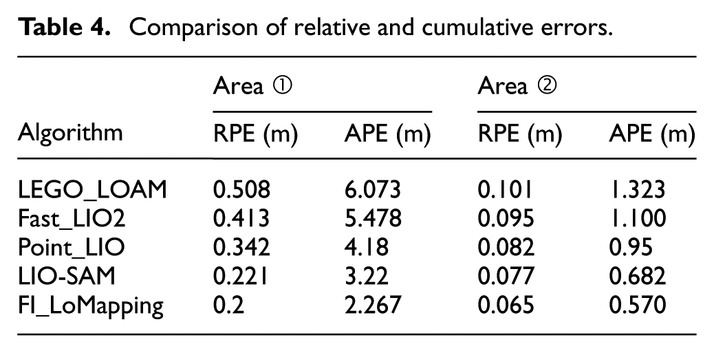
The Root Mean Square Error (RMSE) values of relative position error (RPE shift) and absolute position error (APE) for the five algorithms are listed in Table 4. It can be seen that, compared to the LEGO_LOAM algorithm, the relative and cumulative errors of FI_LoMapping algorithm are reduced by 0.308 and 3.770 m in region ①, and by 0.036 m and 0.753 in region ②, respectively. Compared to the LIO-SAM algorithm, the relative and cumulative errors of the FI_LoMapping algorithm are reduced by 0.0.21 and 0.953 m in region ① and by 0.012 and 0.112 m in region ②, respectively. The results prove that FI_LoMapping can further improve the accuracy of the system and its ability to operate stably in large scenarios, both in cases with more structured information, as region ①, as well as in scenarios with less structured information, as region ②.
Comparison of relative and cumulative errors.
The point cloud maps constructed by FI_LoMapping, Fast_LIO2 and LEGO_LOAM in Region ① and their local details are shown in Figure 13. It can be seen that the point cloud maps, constructed by the multi-sensor tightly coupled SLAM, proposed in this paper, shows high consistency with the actual environment, while features, such as walls and tree trunks, under the local maps, do not have problems, such as ghosting and blurring.
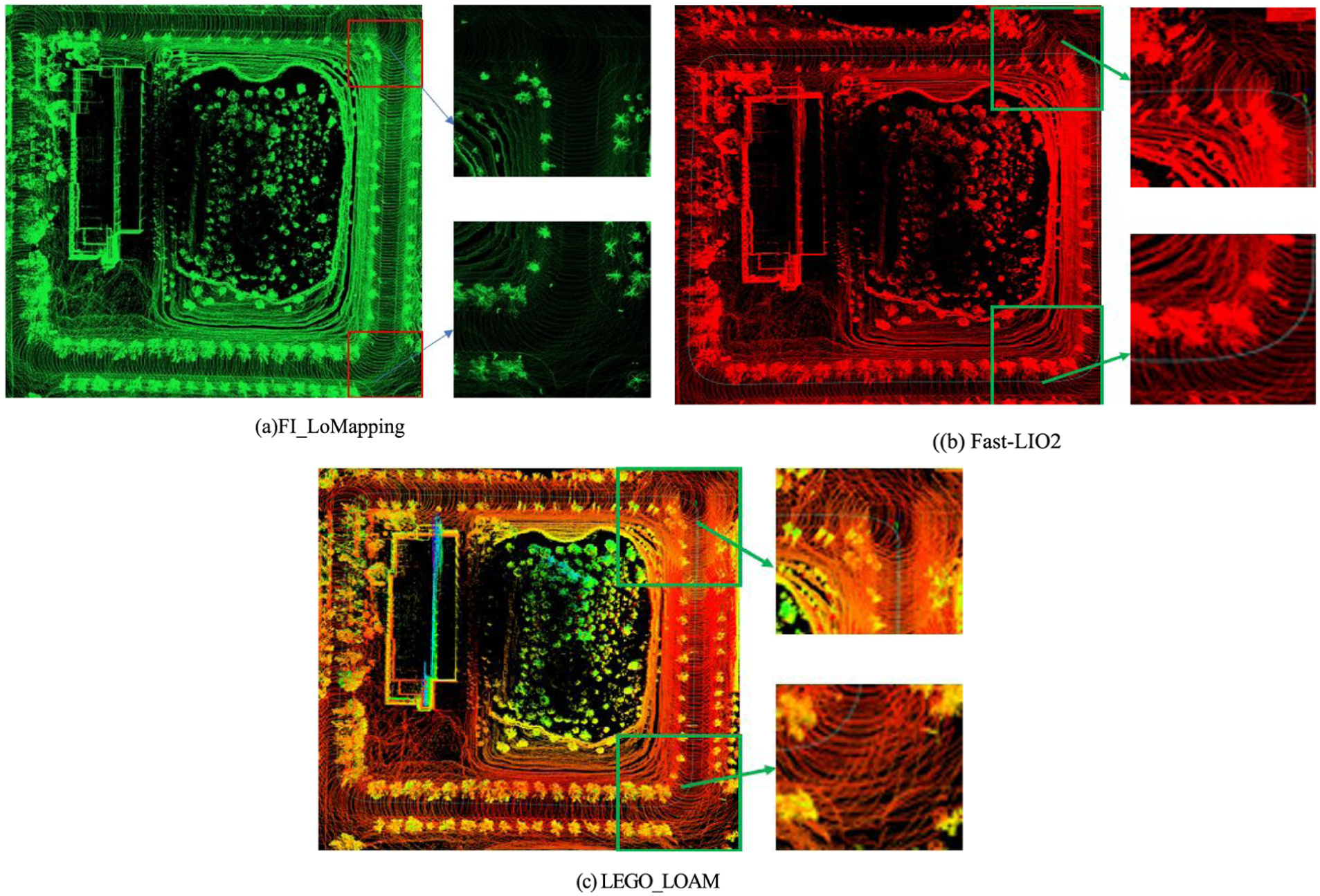
Top view of point cloud in area ① and localization: (a) FI_LoMapping, (b) Fast-LIO2 and (c) LEGO_LOAM.
In region ② with distinct structured features, the point cloud map its detailed parts established by FI_LoMapping algorithm is shown in Figure 14. It can be seen that the constructed 3D point cloud map has a high degree of consistency with the actual environment. The walls in the local map do not have ghosting due to inaccurate positioning, and the features such as tree trunks on both sides of the road do not appear blurry problem. The above experiments indicate that the FI_LoMapping algorithm has high map construction and localization performance in both structured and unstructured scenarios.
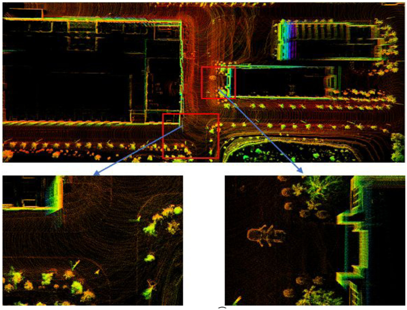
Top view of point cloud in area ② and localization.
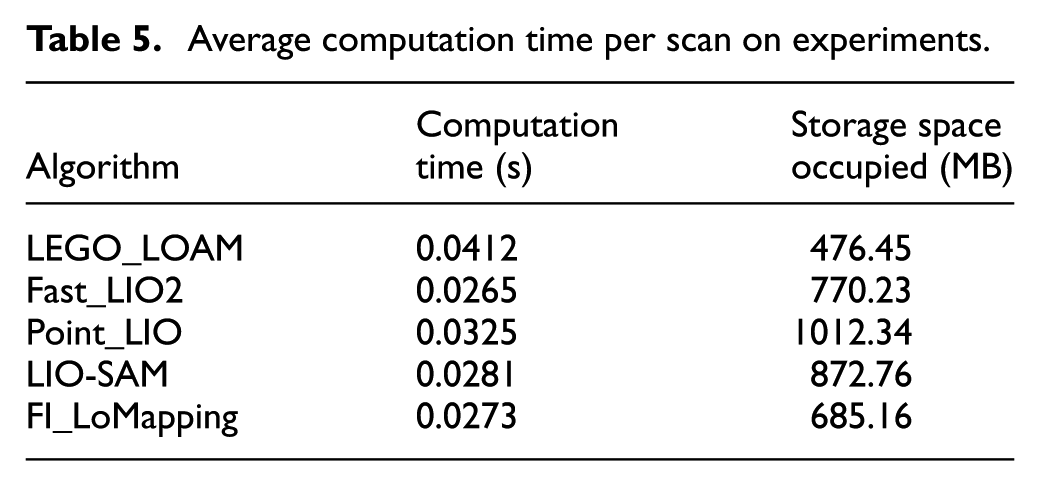
To test the real-time performance of the proposed method on computing platform, we calculated the average computation time per scan of FI_LoMapping, Fast-LIO2, LEGO_LOAM, Point_LIO, LIO-SAM and the results are shown in Table 5. Although Fast-LIO2 achieves optimal time efficiency, the storage space occupied by the algorithm is relatively large, reaching 770.23 MB. The proposed method is fully run in real-time for all the experiments, with competitive performance at around 36 Hz. In addition, the average computation time of FI_LoMapping on experiments is 0.0273 s, as shown in Figure 15. Compared with LEGO_LOAM, Point_LIO, our method demonstrates significant advantages in terms of time efficiency. Similar to FI_LoMapping, LIO-SAM also employs factor graph optimization, and its computation time and memory footprint are basically on the same level.
Average computation time per scan on experiments.
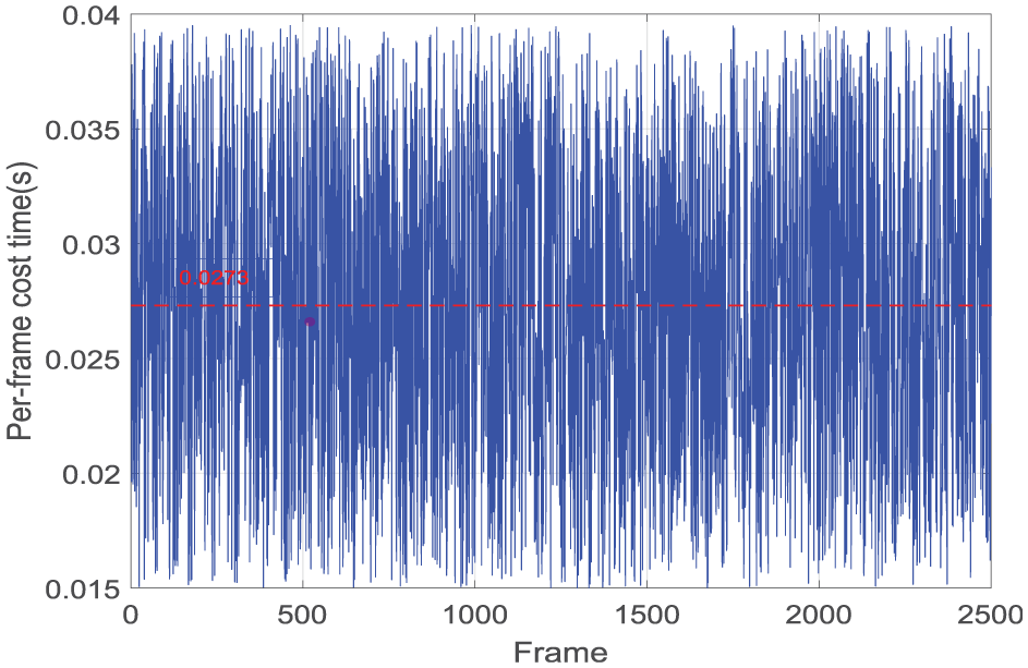
Per-frame cost time of FI_LoMapping.
In complex environments, complex trajectories with emergency turns and U-turns were selected for testing, including structured features such as asphalt roads and buildings, as well as unstructured features such as trees and lakes. In addition, the test trajectory also includes challenging conditions such as emergency left and right turns, right angle turns, and stationary U-turns. The trajectory recorded by INS/RTK in the experiment and the trajectory output by FI_LoMapping Algorithm are shown in Figure 16. It can be seen that in straight road sections, the output trajectory of Algorithm FI_LoMapping is close to INS/RTK. However, there is a certain positioning error during the turning process, mainly caused by the lack of environmental features and IMU drift. This situation is consistent with the simulation results.
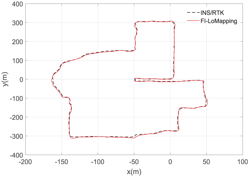
The output trajectory of FI_LoMapping.
In the experiment, compared with INS/RTK devices with high-precision positioning, the positioning error of FI_LoMapping Algorithm in each frame is shown in Figure 17. It can be seen that the maximum error in the entire experiment is 0.634 m, with a variance of 0.0262 m2 and a standard deviation of 0.162 m. This reflects that FI_LoMapping algorithm has high positioning stability and accuracy in complex environments containing structured and unstructured features.
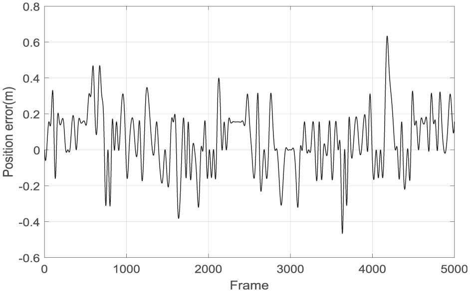
Positioning errors of FI_LoMapping.
Conclusions
In this paper, a SLAM method for tightly coupling lidar and inertial measurement units for different structured feature environments, is presented. Firstly, the extraction of corner and plane point features from LiDAR point clouds and IMU attitude estimation methods have been proposed. On this basis, a perturbation model-based method for detecting environmental degradation is proposed, and the feature value threshold closely related to the environment is derived and calculated. Secondly, a hybrid scanning matching algorithm based on scene judgment is proposed. According to the different feature information in the actual environment, the richness of structured information is used as the basis for judgment and the ICP algorithm that introduces distribution shape constraints is fused with the feature-based point cloud alignment algorithm. In addition, the distribution shape constraint factor is introduced in the feature-lacking scenario to effectively solve the problem of low matching accuracy. Finally, four algorithms were simulated and tested in the KITTI dataset and actual road environments. The experimental results show that the trajectory of FI_LoMapping on straight road sections is close to high-precision INS/RTK, and the positioning error standard deviation of the algorithm is 0.162 m under turning and U-turning conditions, which can meet the application requirements of autonomous vehicles and ground mobile robots. If the existing SLAM systems do not have appropriate strategies to correct feature matching errors, it will increase localization errors and lead to mapping failures. Therefore, in future work, how to build more robust frameworks to discover and remove mismatches is the focus of further research on SLAM system.
Footnotes
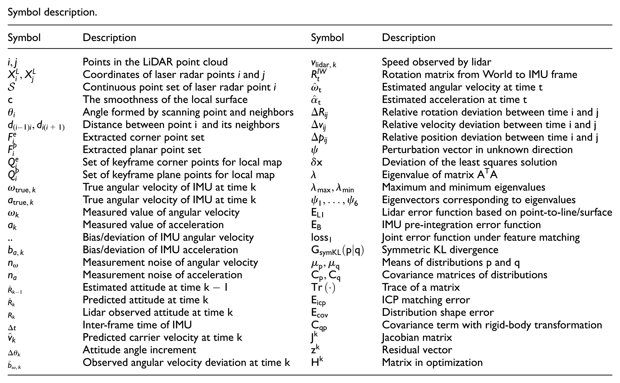
Appendix 1
Symbol description.
| Symbol | Description | Symbol | Description |
|---|---|---|---|
| Points in the LiDAR point cloud | Speed observed by lidar | ||
| Coordinates of laser radar points i and j | Rotation matrix from World to IMU frame | ||
| Continuous point set of laser radar point i | Estimated angular velocity at time | ||
| The smoothness of the local surface | Estimated acceleration at time | ||
| Angle formed by scanning point and neighbors | Relative rotation deviation between time and | ||
| Distance between point and its neighbors | Relative velocity deviation between time and | ||
| Extracted corner point set | Relative position deviation between time and | ||
| Extracted planar point set | Perturbation vector in unknown direction | ||
| Set of keyframe corner points for local map | Deviation of the least squares solution | ||
| Set of keyframe plane points for local map | Eigenvalue of matrix | ||
| True angular velocity of IMU at time | Maximum and minimum eigenvalues | ||
| True angular velocity of IMU at time | Eigenvectors corresponding to eigenvalues | ||
| Measured value of angular velocity | Lidar error function based on point-to-line/surface | ||
| Measured value of acceleration | IMU pre-integration error function | ||
| .. | Bias/deviation of IMU angular velocity | Joint error function under feature matching | |
| Bias/deviation of IMU acceleration | Symmetric KL divergence | ||
| Measurement noise of angular velocity | Means of distributions and | ||
| Measurement noise of acceleration | Covariance matrices of distributions | ||
| Estimated attitude at time | Trace of a matrix | ||
| Predicted attitude at time | ICP matching error | ||
| Lidar observed attitude at time | Distribution shape error | ||
| Inter-frame time of IMU | Covariance term with rigid-body transformation | ||
| Predicted carrier velocity at time | Jacobian matrix | ||
| Attitude angle increment | Residual vector | ||
| Observed angular velocity deviation at time | Matrix in optimization |
Appendix 2
Handling Editor: Chenhui Liang
Ethical considerations
We declare that the vehicle testing in the paper did not involve any human participants (e.g. drivers).
Author contributions
Conceptualization, M.Z.; methodology and software, S.F.; validation, S.F. and A.Z.; writing—original draft preparation, M.Z. and S.F.; writing—review and editing, M.Z.; funding acquisition, M.Z. All authors have read and agreed to the published version of the manuscript.
Funding
The authors disclosed receipt of the following financial support for the research, authorship, and/or publication of this article: This work has been supported in part by the University Natural Sciences Research Project of Anhui Province (2024AH040210), Hefei Key Technology Research and Development Project (2023SGJ018), Anhui Province Key Research and Development Plan Project (202304a05020065).
Declaration of conflicting interests
The authors declared no potential conflicts of interest with respect to the research, authorship, and/or publication of this article.
Data availability statement
Data will be made available on request.