Sage Journals: Discover world-class research

Abstract

To address the coupled geometric and deformation errors in RV reducers, this study proposes a high-precision transmission error prediction method using Stacking ensemble learning, overcoming the limitations of rigid assumptions and inefficient finite element analysis. A finite element model incorporating machining errors is built to generate a dataset via Latin hypercube sampling. Then, based on orthogonal experiments and variance analysis methods, eight typical machining errors of the RV reducer were analyzed to identify the three machining errors that have the greatest impact on the peak-to-peak value of the transmission error. On this basis, A Stacking model is then constructed with SVR, XGBoost, RF, and KNN as base learners and XGBoost as the meta-learner. Experimental results show this model increases the determination coefficient R² by 14.3% and reduces RMSE by 27.4% compared to the best single model. Furthermore, it enables an average 52.48% reduction in the transmission error peak-to-peak value, significantly enhancing prediction accuracy and robustness for RV reducer performance optimization.

Keywords

RV reducer transmission error finite element simulation ensemble learning

Introduction

As the core transmission joint of industrial robots, the performance of the RV reducer directly affects the motion accuracy and stability of robots.^1–3 High-end equipment represented by six-axis industrial robots imposes requirements of large transmission ratio and high output torque on RV reducers. To address the shortcomings of traditional reducers such as insufficient transmission ratio and limited output torque, the RV reducer adopts a composite structure of planetary gear transmission and cycloidal pinwheel transmission, combining the advantages of large transmission ratio and high torque output.^4–6 During the assembly process of the RV reducer, machining errors of components (such as pin machining error and crankshaft eccentricity error) will change the geometric relationship and stress state of the RV reducer, resulting in transmission errors,^7–9 which are manifested as motion lag and increased backlash. This further leads to problems such as decreased repeat positioning accuracy, increased trajectory tracking error, and intensified vibration and noise, seriously affecting the operational performance of robots. Taking a certain type of welding robot as an example, measured data show that when the joint transmission error exceeds 15 arcsec, the weld seam trajectory deviation increases by 35%, directly affecting the welding quality. In application scenarios such as precision assembly, transmission errors can also cause inaccurate positioning of the end effector, resulting in assembly failure or product damage. Therefore, studying the influence law of assembly errors on the transmission accuracy of RV reducers and realizing the accurate prediction of transmission accuracy are of great significance for improving the motion performance and operational reliability of industrial robots.^10–12

Currently, three main methods—analytical modeling, numerical simulation, and experimental testing—are adopted to analyze the influence of reducer machining errors on transmission accuracy. In terms of analytical modeling, Xue et al.¹³ established an analytical prediction methodology of the correlation between transmission error and tooth pitch error for face-hobbed hypoid gears. The variable-step Runge-Kutta algorithm was used to solve the dynamic response of the system, revealing the influence law of carrier machining errors in different directions on the dynamic transmission error and meshing force of the system. For numerical simulation, Huang et al.¹⁴ presents a dynamic modeling and response analysis of cracked herringbone gear transmission systems, with consideration of installation errors. Based on orthogonal tests, the axial deviation most sensitive to meshing characteristics was identified from machining errors in different directions. Regarding experimental testing, Palermo et al.¹² proposed a simplified measurement scheme for gear transmission error (TE) based on low-cost digital encoders, and used this scheme to analyze the influence of gear machining errors on TE.

The analytical modeling method can reveal the causal relationships between error sources (such as eccentricity and pitch error) and transmission errors, offers high computational efficiency without requiring complex computational resources, and enables rapid evaluation of error influence laws.^15–17 The numerical simulation method considers nonlinear factors in gear transmission (elastic deformation, backlash, damping) and intuitively demonstrates motion deviations or stress concentrations caused by errors.^18–20 The experimental testing method is based on real data and directly reflects the comprehensive error effects of actual systems.^21–23 However, these methods all have obvious limitations in transmission error prediction: analytical modeling suffers from insufficient accuracy due to simplified assumptions and struggles to handle complex nonlinear problems; numerical simulation has high computational costs and is difficult to support rapid iterative optimization; experimental testing relies on expensive equipment, has a long cycle, and poor applicability in the early design stage. In contrast, the surrogate model-based transmission error prediction method establishes a mathematical mapping between error parameters and transmission responses, enabling fast and high-precision prediction with only a small number of samples. It not only significantly improves computational efficiency but also supports sensitivity analysis and multi-objective optimization. Willecke et al.²⁴ reduced the parameter dimension by constructing a comprehensive gear deviation surface and trained a deep learning model based on 3000 sets of data, realizing super real-time prediction of the loaded transmission error characteristics of gear pairs and significantly enhancing the efficiency optimization capability in the gearbox manufacturing process. Xu et al.²⁵ proposed an improved method based on the Kriging surrogate model and Sobol sensitivity analysis. By replacing time-consuming simulations, screening key parameters, and combining genetic algorithm optimization, the calibration efficiency and accuracy of the dynamic model of multi-stage gearboxes were significantly improved, achieving more accurate prediction of dynamic characteristics. Sakaridis et al.²⁶ adopted a neural network method to predict the static transmission error of spur gears. A three-layer fully connected network model with periodic symmetry was trained using 20,000 sets of physical simulation data containing 17 parameters, achieving an average error of 0.075% on the test set. This verified the reliability of using neural networks instead of traditional nonlinear solvers for modeling gear static responses.

Geometric modeling and dynamic motion simulation of RV reducer

The RV reducer is a closed-type compound planetary transmission mechanism composed of two-stage reduction mechanisms: the first-stage reduction mechanism is an involute planetary gear mechanism, and the second-stage reduction mechanism is a cycloidal gear-pin gear transmission mechanism. This section mainly conducts geometric modeling and model simplification of the RV reducer to facilitate the subsequent simulation analysis of the entire reducer.

Geometric modeling

Firstly, the overall geometric modeling of the RV reducer is carried out. Its first-stage reduction mechanism is an involute planetary gear mechanism, and the second-stage reduction mechanism is a cycloidal gear-pin gear transmission mechanism. The main structural parameters of the RV reducer are shown in Table 1, and the overall geometric model is illustrated in Figure 1.

Table 1.

Main structural parameters of the RV reducer.

Parameters	Symbol	Value
Module	m	1
Number of teeth of the sun gear	z _s	20
Number of teeth of the synchronizing gear	z _t	28
Number of cycloidal teeth	z _c	39
Number of pin teeth	z _p	40
Short addendum coefficient	K ₁	1.548
Eccentricity	a	3
Pin tooth radius	rrp	8
Radius of the pin tooth distribution circle	r _p	77.5
Cycloidal tooth width	B	10.7

Figure 1.

Geometric model of the RV reducer.

Finite element modeling and dynamic motion simulation

The FEA model in this study is based on the following core assumptions: (a) all materials are homogeneous, isotropic, and linear elastic; (b) gear meshing contact is dry and unlubricated; (c) micro-slip at joint interfaces such as bolt connections is neglected; (d) simulations are conducted under constant rated loads. These assumptions aim to construct a controllable benchmark model for studying the transmission of geometric errors. To reduce the number of meshes in the finite element model and improve computational efficiency, appropriate simplifications are made to the geometric model of the RV reducer in this study, including integrating the crankshaft with the synchronizing gear, removing redundant threaded holes in the geometric model, simplifying the sun gear, synchronizing gear and cycloidal gear, removing the rigid disk, and simplifying the output disk structure. The simplified model of the RV reducer is then imported into finite element preprocessing software for mesh generation. The mesh models of key structures (sun gear, integrated crankshaft and synchronizing gear, cycloidal gear, pins, and pin gear housing) are shown in Figure 2. Among them, the number of meshes for the sun gear finite element model is 19,600, that for the integrated crankshaft and synchronizing gear is 34,490, that for the cycloidal gear is 41,544, and the total number of meshes for the RV reducer finite element model is 368,830. The Overall RV reducer finite element model are shown in Figure 3.

Figure 2.

Finite element models of each component of the RV reducer.

Figure 3.

Overall finite element model of the RV reducer.

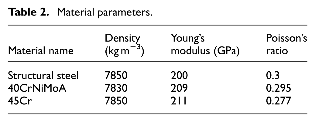
In terms of material settings, the pin gear housing and output disk of the RV reducer are made of structural steel, while structures such as the cycloidal gears, crankshaft, pins, and sun gear are made of 40CrNiMoA alloy steel to meet the requirements of high toughness, fatigue resistance, and mechanical strength. The specific mechanical parameters of each material are detailed in Table 2. The dynamic motion simulation of the RV reducer involves a total of six pairs of contacts: three pairs of contacts between the sun gear and synchronizing gears are set as frictional contacts with a friction coefficient of 0.15; the contacts between the two cycloidal gears and the pin pins are also frictional contacts with a friction coefficient of 0.1; the contacts between the pins and the pin gear housing are set as bonded contacts to facilitate the fixed connection between the pin pins and the pin gear housing. Nine groups of kinematic joints are set to constrain the system motion: 1 fixed joint to ground (for the pin gear housing), 2 revolute joints to ground (for the sun gear and output disk), and 6 body-to-body revolute joints (each cycloidal gear and the crankshaft are equipped with three body-to-body revolute joints). The simulation process is divided into two substeps: in the first substep (0–1 s), the sun gear rotates by 18°, and the output disk is loaded to 100 N m; in the second substep (1–2 s), the load on the output disk remains unchanged, and the sun gear rotates to 180°.

Table 2.

Material parameters.

Material name	Density (kg m⁻³)	Young’s modulus (GPa)	Poisson’s ratio
Structural steel	7850	200	0.3
40CrNiMoA	7830	209	0.295
45Cr	7850	211	0.277

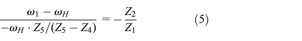
Transmission error calculation

The gear train of RV transmission can be regarded as a planetary closed differential gear train. Here, the planet carrier is denoted by the letter H, and a common angular velocity is applied to the entire gear train, converting the first-stage reduction mechanism of the RV reducer into a fixed-axis gear train. Therefore, the converted transmission ratio of the sun gear and the planetary gear relative to the planet carrier is:

i_{12}^{H} = \frac{ω_{1} - ω_{H}}{ω_{2} - ω_{H}} = - \frac{Z_{2}}{Z_{1}}

(1)

Where: Z₁ is the number of teeth of the sun gear; Z₂ is the number of teeth of the planetary gear; $ω_{1}$ is the angular velocity of the sun gear; $ω_{2}$ is the angular velocity of the synchronizing gear. After adding a virtual common angular velocity of − $ω_{H}$ to the entire transmission gear train, the cycloidal pin gear reduction mechanism can be converted into a differential gear train. The angular velocity of the pin gear is $ω_{5} - ω_{H} = ω_{5}^{H}$ ; the cycloidal gear is restrained by the rotational angular velocity $ω_{2} - ω_{H}$ of the crankshaft and no longer has rotational angular velocity, so $ω_{4}^{H} = 0$ . The center of the cycloidal gear performs circular motion along a guide circle with the eccentricity as the radius centered at the frame, with an angular velocity of $ω_{2}^{H} = ω_{2} - ω_{H}$ . Therefore, at this time, the center of the cycloidal gear can be regarded as being driven to rotate by a carrier $H^{'}$ with an angular velocity of $ω_{H^{'}} = ω_{2} - ω_{H}$ . Substituting into the calculation formula for the transmission ratio of the differential gear train, we obtain:

i_{45}^{H^{'}} = \frac{ω_{4}^{H} - ω_{H^{'}}}{ω_{5}^{H} - ω_{H^{'}}} = \frac{ω_{4}^{H} - (ω_{2} - ω_{H})}{ω_{5}^{H} - (ω_{2} - ω_{H})} = \frac{Z_{5}}{Z_{4}}

(2)

Where: Z₄ is the number of teeth of the cycloidal gear, and Z₅ is the number of teeth of the pin gear.

Furthermore, as $ω_{4}^{H} = 0, ω_{5}^{H} = ω_{5} - ω_{H} = 0 - ω_{H} = - ω_{H}$ , substituting into equation (2) yields:

\frac{0 - (ω_{2} - ω_{H})}{- ω_{H} - (ω_{2} - ω_{H})} = \frac{Z_{5}}{Z_{4}}

(3)

Rearranging gives: $(Z_{5} - Z_{4}) ω_{2} = - Z_{4} \cdot ω_{H}$ , as $Z_{5} - Z_{4} = 1$ ,

ω_{2} = \frac{- Z_{4} \cdot ω_{H}}{Z_{5} - Z_{4}}

(4)

From equations (1) and (3), we obtain:

\frac{ω_{1} - ω_{H}}{- ω_{H} \cdot Z_{5} / (Z_{5} - Z_{4})} = - \frac{Z_{2}}{Z_{1}}

(5)

Since $ω_{H} = ω_{6}$ , therefore, the transmission ratio $i_{16}$ of the RV reducer is:

i_{16} = \frac{ω_{1}}{ω_{6}} = \frac{ω_{1}}{ω_{H}} = 1 + \frac{Z_{2} \cdot Z_{5}}{Z_{1} (Z_{5} - Z_{4})}

(6)

where $ω_{6}$ is the rotational speed of the output shaft. After calculation, the transmission ratio of the RV reducer in this study is 57.

Based on the dynamic motion simulation method of the RV reducer, the rotation angle of the sun gear $θ_{1}$ and the rotation angle $θ_{6}$ of the output disk at different moments are obtained. The transmission error (TE) of the RV reducer is defined as the difference between the actual rotation angle and the theoretical rotation angle of the output disk at different moments, and the calculation formula is as follows:

θ_{TE} = θ_{6} - θ_{1} / i_{16}

(7)

Subsequently, this method can be used to obtain the transmission error data of the RV reducer under different machining errors.

Grid-independence and experimental verification

To balance the efficiency and accuracy of finite element simulation in calculating the transmission error of an RV reducer, this paper refines the contact area of the RV reducer’s finite element model. The sparse grid RV reducer finite element model is shown in Figure 4(a), with a grid count of 208,862. The denser grid RV reducer finite element model is shown in Figure 4(b), with a grid count of 368,830. Based on the method described in Section “Transmission error calculation,” the peak-to-peak transmission error values for the two simulation results are calculated. The peak-to-peak transmission errors are 1.3 and 1.1 arcmin, respectively, and remain unchanged after further grid densification.

Figure 4.

Grid refinement results.

Meanwhile, as shown in Figure 5, this paper also conducted an experiment on the load running-in of the RV reducer under the same load on the test bench. Compared with the measured data of 0.9 arcmin, the refined simulation results are more accurate. Considering the complexity of computer performance and grid division, it is decided to adopt the finite element model with 368,830 grid points as the final finite element model for constructing the surrogate model.

Figure 5.

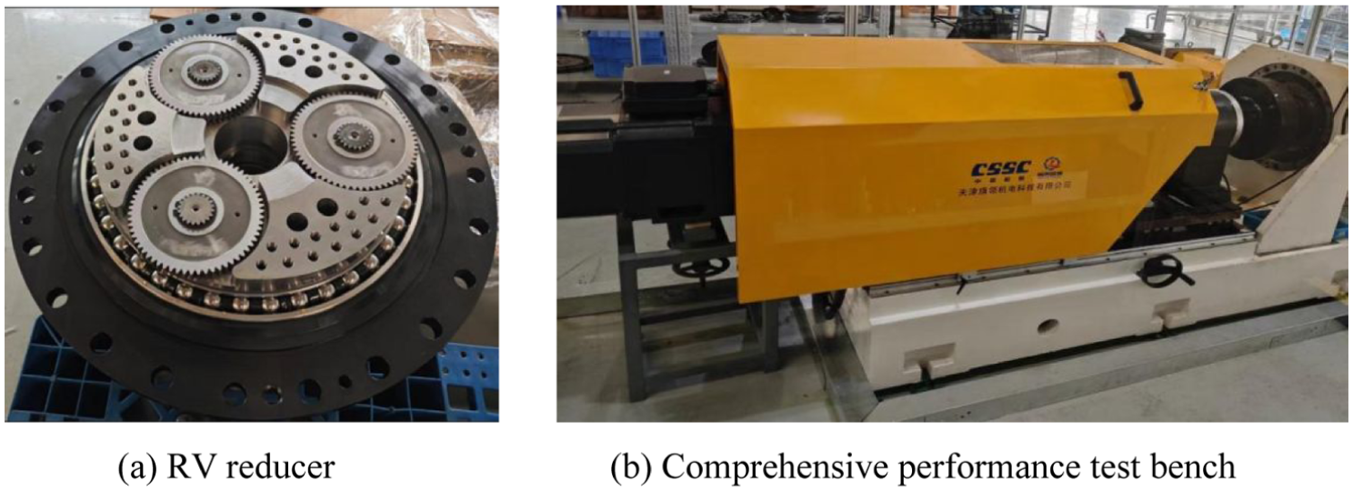
Performance test of RV reducer.

Transmission error prediction of RV reducers based on stacking ensemble learning

The machining errors of RV reducers have a significant impact on transmission errors. This study intends to select eight typical machining errors of RV reducers, conduct a sensitivity analysis, and identify the three machining errors that have the greatest impact on PPSTE from among the eight typical machining errors for the subsequent construction of a surrogate model. The eight selected machining errors are crankshaft eccentricity error and cylindricity errors f_a, f_b, pin gear pin distribution circle radius error and radius errors f_e, f_f, pin gear housing pin hole distribution circle radius error and radius errors f_c, f_d, and cycloid wheel bearing hole distribution circle error and radius errors f_g, f_h. Finally, three typical machining errors are selected, samples are taken within their tolerance ranges, and the corresponding peak-to-peak transmission error values are obtained through the dynamic motion simulation method described in Section “Geometric modeling and dynamic motion simulation of RV reducer” to construct a dataset. Subsequently, a high-precision and robust Stacking ensemble learning model is constructed to achieve accurate prediction of transmission errors of RV reducers.

Definition of machining error and sensitivity analysis

Based on the definition of machining errors and analysis of long-term engineering practice and manufacturing process capabilities, this study defines and assigns tolerances to the following eight basic machining errors. The crankshaft eccentricity error and cylindricity error f_a and f_b are defined as 0–0.02 mm; the distribution circle radius error and radius error f_c and f_d of the pin hole in the pin gear housing are defined as 0–0.02 mm; the manufacturing error of the distribution circle radius error f_e and pin gear pin radius f_f is defined as 0–0.02 mm; the distribution circle error and radius error f_g and f_h of the cycloid bearing hole are defined as 0–0.02 mm.

The influence of eight machining error factors on PPSTE was analyzed using orthogonal experimental design. According to the manufacturing tolerance standards for RV reducers, three levels were set for each factor: eccentricity of 0, 0.01, and 0.02 mm, as shown in Table 3.

Table 3.

Orthogonal experiment table.

Serial number	f _a	f _b	f _c	f _d	f _e	f _f	f _g	f _h	y _i
1	0	0	0	0	0	0	0	0	0.52
2	0	0	0	0.01	0.01	0.01	0.02	0.02	0.66
3	0	0	0	0.02	0.02	0.02	0.01	0.01	1.30
4	0	0.01	0.02	0	0.01	0.02	0	0.01	1.92
5	0	0.01	0.02	0.01	0.02	0	0.02	0	1.53
6	0	0.01	0.02	0.02	0	0.01	0.01	0.02	1.69
7	0	0.02	0.01	0	0.02	0.01	0	0.02	0.99
8	0	0.02	0.01	0.01	0	0.02	0.02	0.01	1.13
9	0	0.02	0.01	0.02	0.01	0	0.01	0	1.04
10	0.01	0	0.02	0	0.02	0.01	0.02	0.01	0.91
11	0.01	0	0.02	0.01	0	0.02	0.01	0	1.49
12	0.01	0	0.02	0.02	0.01	0	0	0.02	1.89
13	0.01	0.01	0.01	0	0	0	0.02	0.02	0.53
14	0.01	0.01	0.01	0.01	0.01	0.01	0.01	0.01	0.75
15	0.01	0.01	0.01	0.02	0.02	0.02	0	0	1.91
16	0.01	0.02	0	0	0.01	0.02	0.02	0	1.51
17	0.01	0.02	0	0.01	0.02	0	0.01	0.02	1.03
18	0.01	0.02	0	0.02	0	0.01	0	0.01	0.55
19	0.02	0	0.01	0	0.01	0.02	0.01	0.02	1.40
20	0.02	0	0.01	0.01	0.02	0	0	0.01	1.17
21	0.02	0	0.01	0.02	0	0.01	0.02	0	1.32
22	0.02	0.01	0	0	0.02	0.01	0.01	0	0.77
23	0.02	0.01	0	0.01	0	0.02	0	0.02	1.47
24	0.02	0.01	0	0.02	0.01	0	0.02	0.01	0.86
25	0.02	0.02	0.02	0	0	0	0.01	0.01	0.73
26	0.02	0.02	0.02	0.01	0.01	0.01	0	0	0.68
27	0.02	0.02	0.02	0.02	0.02	0.02	0.02	0.02	1.07

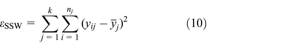
Next, hypotheses are proposed. The null hypothesis (H₀): different levels of each processing error factor have no significant effect on PPSTE; the alternative hypothesis (H₁): at least one different level of a processing error factor has a significant effect on PPSTE. Then, the total sum of squares ( $ε_{SST}$ ) of the eight factors, the between-group sum of squares ( $ε_{SSB}$ ) and the within-group sum of squares ( $ε_{SSW}$ ) are calculated separately, with the following formulas:

ε_{SST} = \sum_{i = 1}^{n} {(y_{i} - \bar{y})}^{2}

(8)

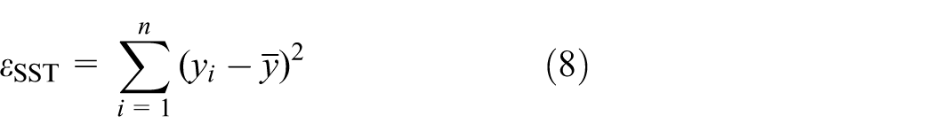
In the formula: n represents the number of trials; y_i denotes the observed value of the ith trial, and y is the mean of all trial observations y_i.

ε_{SSB} = \sum_{j = 1}^{k} n_{j} {({\bar{y}}_{j} - \bar{y})}^{2}

(9)

In the formula: $n_{j}$ is the sample size of group j; ${\bar{y}}_{j}$ is the average observed value of group j; k is the number of groups, and in this experiment, k = 8.

ε_{SSW} = \sum_{j = 1}^{k} \sum_{i = 1}^{n_{j}} {(y_{ij} - {\bar{y}}_{j})}^{2}

(10)

In the formula, $y_{ij}$ represents the ith observation value of the jth group, and ${\bar{y}}_{j}$ represents the average of the observation values in the jth group. The total sum of squares can be decomposed into the between-group sum of squares and the within-group sum of squares:

ε_{SST} = ε_{SSB} + ε_{SSW}

(11)

In the formula, $y_{ij}$ represents the ith observation value of the jth group, and ${\bar{y}}_{j}$ denotes the average of the observation values in the jth group. The total sum of squares can be decomposed into the between-group sum of squares and the within-group sum of squares:

ε_{SST} = ε_{SSB} + ε_{SSW}

(12)

Then, the between-group mean square ( $δ_{MSB}$ ) and within-group mean square ( $δ_{MSW}$ ) are calculated based on the between-group sum of squares and within-group sum of squares, respectively. The F statistic is then calculated based on the ratio of the two, using the following formula:

δ_{MSB} = \frac{δ_{SSB}}{d_{fb}}

(13)

In the formula, $d_{fb}$ represents the between-group degree of freedom.

δ_{MSW} = \frac{δ_{SSW}}{d_{fw}}

(14)

In the formula: $d_{fw}$ represents the within-group degrees of freedom. The between-group degrees of freedom for a single factor is the number of levels minus 1:

d_{fb} = m - 1

(15)

In the formula, m represents the level number. The within-group degrees of freedom $d_{fw}$ are calculated by subtracting the total between-group degrees of freedom from the sample degrees of freedom

d_{fw} = n - 1 - \sum_{k = 1}^{8} d_{fb}^{k}

(16)

The formula for calculating the F statistic is

F = \frac{δ_{MSB}}{δ_{MSW}}

(17)

Finally, given a significance level $α = 0.05$ , the F critical value is determined by referring to the F distribution numerical table based on the total between-group degrees of freedom $d_{fb} = 2$ and within-group degrees of freedom $d_{fw} = 10$ . The significance probability, p value, represents the probability of observing the current F value or a more extreme value under the null hypothesis:

P = P (F \geq F_{0.05} (2, 10))

(18)

The results of the variance analysis are presented in Table 4. According to the variance analysis results, the radius deviation of the pin gear, f_f (F = 15.8, p = 0.002128), the eccentricity error of the crankshaft, f_a (F = 12.87, p = 0.00171), and the radius error of the pin gear distribution circle, f_e (F = 4.86, p = 0.03354), have a significant impact on PPSTE, while the other five factors have a relatively minor influence. The three most significant transmission errors determined for the RV reducer transmission error are the radius deviation of the pin gear, f_f, the eccentricity error of the crankshaft, f_a, and the radius error of the pin gear distribution circle, f_e. These three machining errors will be used for the subsequent construction of the RV reducer transmission error proxy model.

Table 4.

Analysis of variance results.

Machining error	d _fb	d _fw	F	p
f _a	2.0	10	12.867173	0.001716
f _b	2.0	10	0.1824283	0.835425
f _c	2.0	10	0.1382143	0.846189
f _d	2.0	10	0.1955464	0.885346
f _e	2.0	10	4.859281	0.03354
f _f	2.0	10	15.800803	0.002128
f _g	2.0	10	0.1778143	0.869542
f _h	2.0	10	0.5355522	0.925814

The transmission precision of RV reducers largely depends on the manufacturing precision of their core components. Among various manufacturing error sources, the machining error of the pin hole system on the pin gear housing, the dimensional error of the pin pins themselves, and the eccentricity error of the crankshaft are the most critical factors affecting meshing quality. Based on long-term engineering practice and analysis of manufacturing process capability, this study defines the following three basic machining errors and assigns their tolerances as follows:

As an intermediate transmission component between the cycloidal gear and the pin gear housing, the machining error of the pin pins causes problems such as unbalanced load distribution, increased transmission backlash, and intensified vibration and noise. To ensure a good fit of the meshing pair, the manufacturing tolerance for the radius of the pin pins is defined as 0–0.01 mm.The eccentricity of the crankshaft is a core kinematic parameter that determines the correct meshing relationship between the cycloidal gear and the pin pins. If its precision is not guaranteed, the ideal meshing state will be destroyed, which may lead to overload of some tooth surfaces, accelerated wear, or even the occurrence of interference. For this reason, the manufacturing tolerance for the eccentricity is defined as 0–0.015 mm. The radius of the pin distribution circle refers to the radius of the ideal circle where the centers of all pin holes on the pin gear housing are located. If there is an error in the radius of the distribution circle, it will systematically displace the meshing positions of all pin teeth, which is equivalent to changing the theoretical center distance between the cycloidal gear and the pin gear housing, thereby exerting an overall impact on transmission precision and torsional stiffness. Based on the high-precision coordinate boring or the process capability of machining centers for the pin gear housing, the manufacturing tolerance for the radius of the pin distribution circle is defined as 0–0.02 mm.

Stacking ensemble learning method

Stacking (Stacked Generalization) is a heterogeneous ensemble learning framework that was first proposed by Wolpert in 1992.^19,20 Its core idea is to achieve hierarchical fusion of prediction results through a two-layer model architecture: Base-learners generate diverse prediction outputs in the first layer, while the Meta-learner constructs an optimal combination strategy based on the outputs of the Base-learners in the second layer. The Stacking ensemble learning framework has demonstrated stronger generalization potential in dealing with complex nonlinear relationships. The algorithm flow of Stacking ensemble learning is shown in Figure 6, which includes the following steps:

Step 1: Data Preparation. Divide the original dataset into a Train Set and a Test Set, where the Train Set is used to train the model, and the Test Set is used to evaluate the model accuracy.

Step 2: Train Base-learners. First, select multiple different machine learning algorithms as base-learners (e.g. Support Vector Machine (SVM), K-Nearest Neighbors (KNN), Random Forest (RF), etc.). These base-learners can be combinations of different parameters of the same type of algorithm or combinations of different types of algorithms. Next, split the Train Set into K folds (K-Fold). For each base-learner, use K−1 folds to train the model in turn, and use the trained model to make predictions on the remaining 1 fold. Repeat this process K times to ensure each fold is predicted exactly once, then combine the prediction results of all folds to generate the prediction results of the base-learner on the Train Set. Finally, retrain each base-learner using the complete Train Set, and use the trained base-learners to make predictions on the Test Set to generate the prediction results of the Test Set.

Step 3: Train the Meta-learner. First, take the aforementioned prediction results as new features and combine them column-wise to form a Meta-training Set. Next, select several machine learning algorithms as meta-learners (e.g. Linear Regression (LR), Logistic Regression, Gradient Boosting Decision Tree (GBDT), etc.). The task of the meta-learner is to generate the final prediction based on the prediction results of the base-learners. Finally, train the meta-learner using the Meta-training Set.

Step 4: Evaluation of Prediction Results. Combine the prediction results of each base-learner on the Test Set column-wise to form a Meta-test Set. Input the Meta-test Set into the trained meta-learner to generate the final prediction results. Use the true labels of the Test Set and the final prediction results to calculate the model’s prediction performance metrics, such as the coefficient of determination (R²), Root Mean Square Error (RMSE), etc.

Figure 6.

Stacking ensemble learning workflow.

Selection of base-learners and meta-learner

In the selection of base-learners, comprehensive consideration is given to algorithm diversity and performance balance. Support Vector Regression (SVR), eXtreme Gradient Boosting (XGBoost), Light Gradient Boosting Machine (LightGBM), Random Forest (RF), and K-Nearest Neighbors (KNN) are selected as base-learners. These algorithms exhibit significant differences in hypothesis space, optimization objectives, and data sampling, enabling them to provide differentiated and complementary predictive features. For the selection of meta-learners, three algorithms—XGBoost, CatBoost, and LightGBM—are adopted. Through their unique modeling strategies (such as complex interaction learning, local dependency capture, and global-local pattern correlation mining), they effectively integrate the outputs of the base models. Meanwhile, an overfitting prevention mechanism is established to ensure the model has excellent generalization ability. All base models ensure the consistency of prediction accuracy through cross-validation, avoiding interference from noise of weak models on the ensemble effect.

Dataset construction and model training

First, 60 sets of machining error data of RV reducers are obtained through Latin Hypercube Sampling (LHS). The manufacturing tolerance for the pin radius is defined as 0–0.01 mm, the manufacturing tolerance for the eccentricity is 0–0.015 mm, and the manufacturing tolerance for the radius of the pin distribution circle is 0–0.02 mm. The corresponding peak-to-peak values of transmission error are acquired based on dynamic simulation. A 5-fold cross-validation strategy is adopted to train four base-learners (SVR, XGBoost, RF, and KNN) to generate the meta-training set and meta-test set. The diversity of the base-learners is double guaranteed by the differences in algorithm principles and the correlation analysis of prediction results, ensuring the effectiveness of the ensemble model. At the meta-learner layer, XGBoost, CatBoost, and LightGBM are trained respectively. The hyperparameters of all models are systematically optimized through Bayesian optimization to ensure the optimal prediction performance of the models. To combat the risk of overfitting in small sample sizes, we divided all data into a training set (70%) and an independent test set (30%). All performance metrics are based on the test set that was not involved in training, objectively reflecting the model’s generalization ability. We adopted a 5-fold cross-validation strategy to train four base learners: SVR, XGBoost, RF, and KNN, generating meta-training sets and meta-test sets. The diversity of the base learners is ensured through both algorithmic principle differences and predictive result correlation analysis, ensuring the effectiveness of the ensemble model. At the meta-learner layer, XGBoost, CatBoost, and LightGBM were used for training. All models’ hyperparameters were tuned through a Bayesian optimization system to ensure optimal predictive performance. Finally, the prediction performance of the model is evaluated by indicators such as RMSE, Mean Absolute Percentage Error (MAPE), and R², and compared with individual base-learners for verification. The calculation formulas of the indicators are as follows:

χ_{R^{2}} = 1 - \frac{\sum_{i = 1}^{n} {(y_{i} - f (x_{i}))}^{2}}{\sum_{i = 1}^{n} {(y_{i} - \bar{y})}^{2}}

(19)

χ_{RMSE} = \sqrt{\frac{1}{n} \sum_{i = 1}^{n} {(y_{i} - f (x_{i}))}^{2}}

(20)

Where: n is the number of samples in the test set; y_i is the true peak-to-peak value of transmission error; $\bar{y}$ is the mean value of y_i. f(x_i) is the predicted peak-to-peak value of transmission error. Finally, calculate the Mean Absolute Percentage Error (MAPE):

χ_{MAPE} = \sum_{i = 1}^{n} | \frac{y_{i} - f (x_{i})}{y_{i}} | \times 100 %

(21)

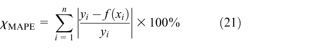
through the aforementioned indicators, the prediction accuracy and generalization ability of the model are verified.

Discussion and analysis of results

Using the aforementioned process, the Stacking ensemble learning model is trained, and the prediction results of the four base-learners (SVR, XGBoost, RF, and KNN) as well as the Stacking ensemble model on the training set and test set are obtained. With the sorted sample indices as the horizontal axis, the variation curves of the true values and the predicted values of each model are plotted, as shown in Figure 7. In the visualization graph, the base-learners are represented by dashed lines with medium transparency to reflect the prediction fluctuations of individual models; the Stacking ensemble model uses solid lines with increased line width to highlight the stable trend after integration; the true values are used as the reference benchmark, represented by black thick solid lines with dot markers. It can be observed from the figure that the prediction trajectories of individual base-learners show obvious oscillatory deviations (e.g. local overfitting or underfitting), while the curve of the ensemble model is closer to the true values in the overall trend with a smaller fluctuation range.

Figure 7.

Comparative analysis of training set prediction.

By comparing the prediction performance of each base-learner and the three Stacking ensemble models on the test set, as shown in Figure 8, the prediction trajectories of the base-learners (SVM, KNN, XGBoost, RF, represented by dashed lines) generally exhibit relatively large fluctuations. In contrast, the three Stacking models using XGBoost, CatBoost, and LightGBM as meta-learners (represented by solid lines) demonstrate better fitting characteristics, and the degree of overlap between their prediction curves and the true value trajectory is significantly improved.

Figure 8.

Comparative analysis of test set prediction.

The prediction results of different base-learners and the final ensemble learning model are shown in Table 5. First, comparing the ensemble models with different meta-learners, the Stacking_XGB model (using XGBoost as the meta-learner) performs the best among the three indicators. Compared with the second-ranked Stacking_LGB (using LightGBM as the meta-learner), its R² increases by 14.4%, while RMSE and MAPE decrease by 27.5% and 27.0% respectively. This indicates that the Stacking_XGB model, through the unique regularization terms and boosting mechanism of XGBoost, effectively integrates the nonlinear feature capture capabilities of base-learners such as SVM and KNN, demonstrating stronger generalization performance in handling complex data relationships.

Table 5.

Prediction accuracy metrics of the model.

Model	$χ_{R^{2}}$	$χ_{RMSE}$	$χ_{MAPE}$
SVM	0.7680	36.2554	12.10
XGB	0.6629	43.6958	15.69
LGB	0.6619	43.7609	15.20
KNN	0.7635	36.6013	12.04
RF	0.6757	42.8615	15.52
Stacking_LGB	0.7671	36.3206	12.54
Stacking_CAT	0.7185	39.9339	13.52
Stacking_XGB	0.8775	26.3373	9.16

Second, among the individual base-learners, SVM performs the best in terms of R² and RMSE. The Stacking_XGB model increases R² by 14.3% and decreases RMSE by 27.4% compared with SVM. KNN performs the best in terms of MAPE, and the Stacking_XGB model reduces MAPE by 23.9% compared with KNN. This leapfrog performance improvement fully verifies the significant advantages of the ensemble learning model. The base-learner layer achieves multi-angle coverage of the feature space through diverse modeling strategies such as SVM and KNN, while the meta-learner layer effectively suppresses the overfitting tendency of individual models through the gradient boosting mechanism of XGBoost, ultimately achieving a significant improvement in prediction accuracy. It should be noted that the maximum value of R² in the table is 0.8775. This may be due to insufficient training data, which prevents the model from fully capturing complex nonlinear features, resulting in some overfitting. At the same time, finite element simulation itself is an approximation of “real physics” and involves some simplifications (such as ignoring lubricating oil films, microscopic surface morphology, etc.). These unsimulated physical factors also contribute to part of the prediction deviation.

Transmission error optimization of RV reducers based on differential evolution algorithm

Differential Evolution (DE) is a population-based heuristic search algorithm for solving continuous optimization problems. Proposed by Rainer Storn and Kenneth Price in 1995, it is inspired by genetic algorithms but adopts unique mutation and crossover mechanisms. The overall flow of the differential evolution algorithm is shown in Figure 9, which mainly includes the following five steps:

(1) Initialize the population as: ${\begin{matrix} X_{i} (0) | x_{i, j}^{L} ⩽ x_{i, j} (0) ⩽ x_{i, j}^{U}; i = 1, 2, \dots, NP; j = 1, 2, \dots, D \end{matrix}}$ , then randomly generate each individual in the population using the following formula:

x_{j, i} (0) = x_{j, i}^{L} + rand (0, 1) \cdot (x_{j, i}^{U} - x_{j, i}^{L})

(22)

Where $X_{i} (0)$ represents the ith individual of the 0th generation in the population; $x_{j, i} (0)$ represents the jth gene of the ith individual in the 0th generation; NP is the population size; $rand (0, 1)$ represents a random number uniformly distributed over the interval (0, 1).

(2) Mutation: Mutation operation is an important operation of the differential evolution algorithm. Individual mutation is achieved through differential operation: randomly select two different individuals from the population, scale their vector difference, and then perform vector synthesis with the individual to be mutated. Common differential strategies are as follows:

\begin{matrix} v_{i} (g + 1) = x_{i_{1}} (g) + F \cdot (x_{i} (g) - x_{ij} (g)) \\ i \neq r_{1} \neq r_{2} \neq r_{3} \end{matrix}

(23)

Where F is the scaling factor, and $x_{i} (g)$ represents the ith individual in the population of the gth generation. In the process of evolution, it is also necessary to ensure the validity of the newly generated solutions. Therefore, it is essential to judge whether the generated solutions satisfy the boundary conditions; if not, they need to be regenerated. The population of the gth generation can be expressed as:

{x_{i} (g) | x_{j, i}^{L} ⩽ x_{j, i} (g) ⩽ x_{j, i}^{v}, i = 1, 2, \dots, NP; j = 1, 2, \dots, D}

(24)

The gth generation population after mutation can be expressed as:

\begin{matrix} {x_{i} (g + 1) | x_{j, i}^{L} ⩽ x_{j, i} (g + 1) ⩽ x_{j, i}^{v}, i = 1, 2, \dots, NP; j = 1, 2, \dots, D} \end{matrix}

(25)

(3) Crossover: Perform crossover using the gth generation population and the mutation intermediates. The process can be expressed as:

u_{j, i} (g + 1) = \begin{matrix} v_{j, i} (g + 1), if rand (0, 1) ⩽ CR or j = j_{rand} \\ x_{j, i} (g), otherwise \end{matrix}

(26)

Where CR is the crossover probability; $j_{rand}$ represents a random integer.

(4) Selection: The greedy algorithm is adopted to select individuals for the next-generation population. The process can be expressed as:

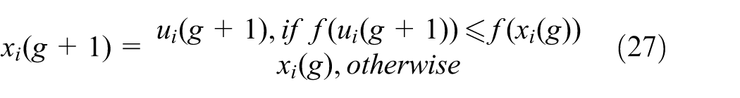
x_{i} (g + 1) = \begin{matrix} u_{i} (g + 1), if f (u_{i} (g + 1)) ⩽ f (x_{i} (g)) \\ x_{i} (g), otherwise \end{matrix}

(27)

(5) Termination Condition: Repeat steps 2–4 until a certain termination condition is met, such as reaching the maximum number of iterations or the quality of solutions meeting the predetermined threshold.

Based on the ensemble learning model with the highest prediction accuracy in Section “Transmission error prediction of RV reducers based on stacking ensemble learning,” the differential evolution algorithm is adopted to optimize machining errors, taking minimizing the peak-to-peak value of transmission error as the objective. The parameters of the optimization algorithm are set as follows: the maximum number of iterations is 1000, the population size is 30, the scaling factor F is determined by the mutation parameter (with a range of (0.5, 1)), the crossover probability CR is set to 0.7, and the convergence tolerance of the algorithm is set to 0.01.

Figure 9.

Overall flow of the differential evolution algorithm.

To demonstrate the accuracy and robustness of the optimization results, we conducted a simple local sensitivity analysis on the optimal tolerance combination obtained through the differential evolution algorithm. We slightly perturbed the error values near the optimal solution and observed the change gradient of PPSTE. The results indicated that PPSTE is relatively insensitive to error changes at the optimal solution, indicating the solution’s robustness. Additionally, four sets of machining errors were randomly generated, and the meshing processes for these four sets were modeled and simulated. PPSTE was calculated and compared with the optimal modification parameters. The modification parameters and their corresponding PPSTE values are presented in Table 6.

Table 6.

Optimized machining errors.

Group number	Pin gear pin radius deviation (mm)	Crankshaft eccentricity error (mm)	Pin gear distribution circle radius deviation (mm)	Peak-to-peak value of transmission error (arcmin)
1	0.02	0.12	0.18	2.3
2	0.05	0.09	0.16	3.1
3	0.03	0.04	0.05	1.9
4	0.07	0.08	0.09	2.8
After optimization	0.02	0.06	0.12	1.2

It can be seen that the transmission error fluctuation of the optimized gear pair is the smallest, with a PPSTE of only 1.2 arcmin. Compared with the gear pairs with the other four sets of machining errors, the PPSTE is decreased by an average of 52.48%, which significantly improves the vibration and noise reduction effect of the gear pair. This verifies the reliability and accuracy of the method proposed in this paper.

Conclusions and prospects

(1) Proposes a high-precision and fast prediction method for the transmission error of RV reducers based on Stacking ensemble learning. The ensemble learning model takes Support Vector Regression (SVR), XGBoost, Random Forest (RF), and K-Nearest Neighbors (KNN) as base learners, with XGBoost serving as the meta-learner. Experimental results show that compared with the optimal single model, the coefficient of determination R² of the ensemble learning model increases by 14.3%, and the root mean square error (RMSE) decreases by 27.4%, effectively addressing the problem of insufficient generalization ability of a single surrogate model.

(2) Adopts the differential evolution algorithm to optimize the machining errors of RV reducers, the peak-to-peak value of the transmission error for the optimized RV reducer was reduced by an average of 52.48%, reducing the peak-to-peak value of the RV reducer’s transmission error and significantly improving the vibration and noise reduction effect. By optimizing the machining errors of the RV reducer using the differential evolution algorithm, the peak-to-peak value of the transmission error of the RV reducer has been reduced, significantly enhancing the shock absorption and noise reduction effects. The core value lies in providing engineers with an efficient “digital testbed,” enabling them to quickly evaluate the final transmission accuracy under different combinations of tolerance levels, thus making the most cost-effective accuracy allocation decisions during the design phase. At the same time, the single-objective optimization presented in this paper has its limitations. Its primary objective is to demonstrate the effectiveness of the proposed framework in minimizing the core indicator of transmission error, laying the foundation for subsequent multi-objective optimization.

(3) By combining finite element simulation and machine learning, a method for predicting transmission errors of spatially driven components has been developed, encompassing geometric modeling, mesh generation, dynamic simulation, and data-driven analysis. This study focuses on geometric errors as the core factor, and does not yet consider complex factors such as clearance, dynamic load changes, friction, and thermal effects. The introduction of these factors would greatly increase model complexity and computational costs. Incorporating the coupled effects of multiple physical fields into consideration is an important direction for future research.

Footnotes

Handling Editor: Cuneyt Fetvaci

ORCID iD

Le Chang

Funding

The authors received no financial support for the research, authorship, and/or publication of this article.

Declaration of conflicting interests

The authors declared no potential conflicts of interest with respect to the research, authorship, and/or publication of this article.

References

Liu

Zhang

Zhu

, et al. State of art of gear contact fatigue theories. J Mech Eng 2022; 58(3): 95–120.

Zhang

Song

Jing

, et al. Displacement prediction and optimization of a non-circular planetary gear hydraulic motor. Adv Mech Eng 2021; 13(11): 16878140211062690.

Al Rifaie

Abdulhadi

Mian

. Advances in mechanical metamaterials for vibration isolation: a review. Adv Mech Eng 2022; 14(3): 16878132221082872.

Riaz

Khan

. A numerical approach to the modeling of Thompson and Troian slip on magnetized flow of Al₂O₃–PAO nanolubricant over an inclined rotating disk. Adv Mech Eng 2023; 15(6): 16878132231183926.

Nie

Chen

Liu

. Research on noise reduction of drive axle hypoid gear based on tooth surface mismatch modification. Adv Mech Eng 2024; 16(2): 16878132241228195.

Zhang

Shi

. Research on friction compensation method of electromechanical actuator based on improved active disturbance rejection control. Actuators 2023; 12(12): 445. https://doi.org/10.3390/act12120445

Chen

. Rounding theory and method for the pitch curves of the variable center distance non-circular gear pair based on working conditions. Adv Mech Eng 2024; 16(4): 16878132241242203.

Tao

Liu

, et al. The effect of cycloid gear wear on the transmission accuracy of the RV reducer. Machines 2024; 12(8): 511.

Zhai

Zhu

Song

, et al. Influences of carrier assembly errors on the dynamic characteristics for wind turbine gearbox. Mech Mach Theory 2016; 103: 138–147.

10.

Liu

Peng

Xiang

, et al. Dynamic characteristics analysis of multi-stage planetary gear system for wind turbines. Acta Energiae Solaris Sinica 2025; 46: 583–590.

11.

Zhao

Yang

, et al. Meshing characteristics of spur gear pairs with tooth modification under different assembly errors and sensitivity analysis for impact factors. J Mech Sci Technol 2023; 37(1): 149–162.

12.

Palermo

Britte

Janssens

, et al. The measurement of gear transmission error as an NVH indicator: theoretical discussion and industrial application via low-cost digital encoders to an all-electric vehicle gearbox. Mech Syst Signal Process 2018; 110: 368–389.

13.

Xue

Liang

Song

, et al. An analytical prediction methodology of the correlation between transmission error and tooth pitch error for face-hobbed hypoid gears. Meccanica 2024; 59(2): 217–233.

14.

Huang

. Dynamic modeling and response analysis of cracked herringbone gear transmission systems with installation errors. Mech Mach Theory 2025; 206: 105924.

15.

Liu

Wang

, et al. Nonlinear dynamics of fault electromechanical coupling transmission system in electrical vehicles. Nonlinear Dyn 2024; 112(17): 14879–14905.

16.

Molaie

Samani

Zippo

, et al. Spiral bevel gears: nonlinear dynamic model based on accurate static stiffness evaluation. J Sound Vib 2023; 544: 117395.

17.

Guangjian

Lin

, et al. Research on the dynamic transmission error of a spur gear pair with eccentricities by finite element method. Mech Mach Theory 2017; 109: 1–13.

18.

Autiero

Paoli

Cirelli

, et al. The effect of different profile modifications on the static and dynamic transmission error of spur gears. Mech Mach Theory 2024; 201: 105752.

19.

Hotait

Kahraman

. Experiments on the relationship between the dynamic transmission error and the dynamic stress factor of spur gear pairs. Mech Mach Theory 2013; 70: 116–128.

20.

Chen

Tang

. Dynamics analysis of a crowned gear transmission system with impact damping: based on experimental transmission error. Mech Mach Theory 2014; 74: 354–369.

21.

Bozca

. Transmission error model-based optimisation of the geometric design parameters of an automotive transmission gearbox to reduce gear-rattle noise. Appl Acoust 2018; 130: 247–259.

22.

Khezri

Schiller

Goka

, et al. Evolutionary cost-tolerance optimization for complex assembly mechanisms via simulation and surrogate modeling approaches: application on micro gears. Int J Adv Manuf Technol 2023; 126(9): 4101–4117.

23.

Meng

Yang

Zhang

, et al. Structural reliability analysis and uncertainties-based collaborative design and optimization of turbine blades using surrogate model. Fatigue Fract Eng Mater Struct 2019; 42(6): 1219–1227.

24.

Willecke

Brimmers

Brecher

. Surrogate model based prediction of transmission error characteristics based on generalized topography deviations. Forsch Ingenieurwes 2023; 87(1): 431–440.

25.

Qin

Liu

, et al. An improved dynamic model updating method for multistage gearbox based on surrogate model and sensitivity analysis. IEEE Access 2021; 9: 18527–18537.

26.

Sakaridis

Kalligeros

Papalexis

, et al. Symmetry preserving neural network models for spur gear static transmission error curves. Mech Mach Theory 2023; 187: 105369.

Method for transmission error prediction and optimization of RV reducer based on ensemble learning

Abstract

Keywords

Introduction

Geometric modeling and dynamic motion simulation of RV reducer

Geometric modeling

Finite element modeling and dynamic motion simulation

Transmission error calculation

Grid-independence and experimental verification

Transmission error prediction of RV reducers based on stacking ensemble learning

Definition of machining error and sensitivity analysis

Stacking ensemble learning method

Selection of base-learners and meta-learner

Dataset construction and model training

Discussion and analysis of results

Transmission error optimization of RV reducers based on differential evolution algorithm

Conclusions and prospects

Footnotes

ORCID iD

Funding

Declaration of conflicting interests

References