A new deep learning model for short term electricity load forecasting using fuzzy granulation and attention mechanism to support clean energy systems

Abstract

Providing accurate electricity load forecasts is crucial for ensuring a cleaner and more sustainable environment, as these forecasts enable the balancing of energy supply and demand, reduce unnecessary reserve capacity requirements and lower dependence on fossil fuels. Objective of this study is to improve the limited performance of existing electricity load forecast models using time series data and to make more accurate forecasts. In this study, the Fuzzy Information Granulation method was applied to Türkiye’s actual hourly electricity load data to enhance the interpretability of time series data and better manage uncertainties. Then, the structure based on the combination of Long-Short-Term Memory encoder and Gated Recurrent Unit decoder structure is hybridized by implementing the Attention Mechanism to increase the ability to focus on the features of time-dependent sequential data. In addition, the Bayesian Optimization method was applied to maximize the performance of the obtained hybrid model and analyze the effects of the model’s hyperparameters on prediction accuracy performance. It is observed that the proposed model outperforms four different benchmark models and provides an improvement in electricity load forecasting by applying the Diebold-Mariano statistical test and 10 different evaluation metrics used to compare the performance of time series forecasting models.

Introduction

The transformation in the energy sector, the increasing use of renewable resources, and the effective management of consumption necessitate the development of accurate electricity load forecasting methods. High-accuracy short- and medium-term load forecasting is essential for the safe and efficient integration renewable energy sources such as solar and wind power. These forecasts play a critical role in the balanced operation of energy systems, production planning, and policy-making processes, and they help maintain grid stability by mitigating the uncertainties introduced by renewable energy. However, the uncertainty and sudden changes inherent in renewable energy sources render classical time series analysis methods inadequate, thereby increasing the need for more advanced, flexible, and data-driven forecasting models. As study ¹ attests, classical models such as ARIMA and Box–Jenkins are based on statistical assumptions and consistent/stationary conditions and perform poorly on complex and noisy data. Considering the structure of energy sources, the importance of more flexible approaches such as deep learning in load forecasting is increasing and becoming widely preferred.

Long Short-Term Memory (LSTM) networks, which are deep learning-based methods, stand out due to their ability to successfully model long-term dependencies in time series data. In the study, ¹ which conducted time series analysis with electricity load data used in Türkiye, the prediction performances of LSTM, Gated Recurrent Unit (GRU), and Convolutional Neural Networks (CNN’s) architectures were compared. As a result, LSTM stood out with the highest accuracy rate. The study emphasized that LSTM, unlike Recurrent Neural Network (RNN) structures, overcomes the vanishing gradient problem, supporting its preference for time series studies. Similarly in Majeed et al., ² as a result of hybridization of RNN structure with LSTM networks in order to prevent the vanishing gradient problem, it was seen that the long-term forecasting performance in load forecasting in energy systems stood out by obtaining the lowest error rate compared to classical RNN, CNN, and GRU models. In study, ³ which used electricity consumption data per household in France, Artificial Neural Network (ANN), CNN, and LSTM-based architectures were compared in a similar manner based on their energy estimation performance. Here, the classical LSTM model was hybridized with the Attention mechanism. As a result, it successfully modeled seasonal cycles and showed statistically significantly higher performance compared to other architectures. This suggests that the LSTM architecture has a flexible structure that can be successfully hybridized with various architectures. Study ⁴ focused on long-term time series forecasting, an LSTM network was also hybridized with an attention mechanism. It was observed that this hybrid model interpreted important information in long sequences more accurately. This study, which achieved a 2%–13% increase in model prediction accuracy, supports the use of LSTM-based hybrid architectures in the energy sector, where predictive power is crucial for effective energy planning.

It is a fact that the classical LSTM network is widely preferred in forecasting studies in the literature due to its successful performance in time series. In addition, thanks to the flexible architecture of LSTM that allows it to be successfully hybridized with different architectures, the number of studies indicating that hybrid LSTM models stand out with their high prediction capabilities has increased considerably in the literature over the years. For this reason, the study ⁵ is another example of the success of the LSTM structure used with the attention mechanism, and in addition, the encoder-decoder architecture in the study was configured with different hidden layers. This developed structure was compared to the classical LSTM and GRU models, yielding more consistent and accurate predictions for 60- and 90-min forecasts. Similarly, in the study, ⁶ it was observed that the use of LSTM-based architecture and the encoder structure hybridized with these architectures increased the prediction success compared to using LSTM alone, thanks to the superior ability of the decoder structure in extracting information from time series, the decoder structure in accessing past and future information, and the attention mechanism in capturing important information that affects accuracy performance. It has also been suggested that this hybrid structure can cope better with noisy data. In study, ⁷ by integrating the Attention mechanism into the LSTM-based deep learning model to predict future sales, a 2.3% Root Mean Squared Error (RMSE) reduction was achieved in forecasting performance, especially in categories with high seasonality and during volatile periods such as holidays.

As another hybrid approach, the study ⁸ shows that using LSTM and GRU architectures together improves prediction performance, especially on complex and noisy data, compared to using LSTM or GRU architectures separately. In the study, ⁹ a sequential hybrid structure was developed for stock price prediction. It first uses the GRU structure to capture short- and medium-term dependencies and then uses the GRU outputs in the LSTM structure to capture long-term dependencies. This hybrid structure provides superior performance compared to classical LSTM and CNN structures, both in terms of ease of hyperparameter tuning and accuracy. In both Yunita et al. ⁸ and Farhadi et al., ⁹ it was observed that using a hybrid with LSTM is more efficient due to the ease provided in the training phase, because GRU has a simpler architecture and fewer parameters than LSTM. In these studies, the hybrid LSTM-GRU model achieved the highest accuracy across various country datasets, proving the model’s effectiveness under different economic conditions. In another study, ¹⁰ the hybrid LSTM-GRU model used for wave height prediction significantly improved prediction performance by reducing the impact of non-stationary patterns. Moreover, in study, ¹¹ this hybrid structure exhibited high reliability with low error rates in both normal and noisy conditions in electric vehicle battery state estimation. These findings reveal that the integration of GRU into LSTM models provides significant contributions in terms of both accuracy and computational efficiency, and hybrid models become a powerful alternative in producing reliable estimations in complex systems such as energy.

There are many other studies in the literature that have observed that the hybridization of the attention mechanism and encoder-decoder structure with various deep learning architectures increases model performance in studies suitable for the purpose of this study. For example, in the model developed by integrating the attention mechanism and CNN into the Bidirectional LSTM-based encoder-decoder structure in Dai et al. ⁶ significant improvements were achieved in both short-term and long-term load estimates. The attention mechanism here increased the overall accuracy of the model by focusing on the effective parts of the input sequences in the estimate. In Zhao et al., ¹² it was stated that the attention mechanism, when used together with LSTM, better models the long-term dependencies in travel time estimates and significantly increases the estimate accuracy. In Pan et al., ¹³ it was shown that the attention mechanism better captures the latent spatial-temporal relationships in oil well production data and significantly improves the estimate performance. In study, ¹⁴ thanks to the attention mechanism, impurity identification in complex texture backgrounds was successfully handled, and an improvement of more than 10% was observed when looking at the F1 score and recall rate. Also, encoder-decoder structure provides an effective transition from the past to the future, allowing better models of long-term dependencies in time series, reducing error propagation and increasing prediction accuracy. For example, in the study, ¹⁵ the GRU network with the encoder-decoder structure was preferred for high accuracy prediction of reheat temperatures of coal-fired power plants. In another case study, ¹⁶ it was observed that by integrating the attention mechanism into the encoder-decoder structure, this hybrid architecture can deal with complex temporal dependencies and patterns in stock price data, thus increasing its modeling ability.

When using deep learning models to make predictions using time series data, dealing with long-term dependencies and ensuring the model accurately interprets these dependencies is more challenging than capturing short-term dependencies. Because as time steps increase, the accumulation of errors will increase, and noise will have an increasingly negative impact on model performance. Therefore, for more consistent and accurate predictions further into the future, it is recommended to use the Fuzzy Information Granulation (FIG) method, which allows time series to be treated as smaller and more meaningful pieces, or granules, in conjunction with deep learning models such as LSTM. The reason why these granules are described as “fuzzy” is that they treat the data as fuzzier categories rather than trying to make sense of it with sharp and clear boundaries, thus enabling a more accurate interpretation of dynamic structures. Thanks to the FIG method, the LSTM model can cope with longer-term dependencies and enable the model to make more consistent predictions.

The study ¹⁷ demonstrates the increased success in prediction performance achieved when the FIG method is used with various architectures. In this study, the attention mechanism was strengthened with the FIG method and hybridized with a GRU-based encoder-decoder structure, thus achieving accurate and consistent prediction success by providing superior success in long-term dependencies as well as short-term dependencies. Also, FIG contributes to more accurate extraction of temporal patterns by adaptively dividing the data according to the distribution properties. In other words, it can be said that noisy and variable data in real-world data becomes more meaningful for deep learning models thanks to the FIG method. In Zhou et al., ¹⁸ the FIG-based model developed for industrial gas demand forecasting has demonstrated the effectiveness of FIG in extracting multi-scale data features. The error correction mechanism used with FIG has increased the reliability especially in long-term forecasts and improved the coverage of forecast intervals. In study ¹⁹ a hybrid model that can provide a balance between forecast accuracy and interpretability was developed by integrating the FIG method into the model applied to improve stock market forecasting. In this way, the model gained the ability to adapt to temporary fluctuations in financial time series by capturing short-term trend dynamics. In study, ²⁰ the trend-based FIG-LSTM model developed in has provided lower error accumulation in long-term forecasts compared to the classical LSTM structure, and thanks to the granular structure of the forecasts, both the accuracy and interpretability of the model have been increased. FIG’s representation of trend information through granules has reduced error propagation in the forecast process and has also strengthened the insight-generating capacity of the model. Similarly, in Zhu et al., ²¹ the FIG-based LSTM model, which takes cyclical patterns into account, reduces the effects of redundancy, noise, and outliers in the data by isolating the periodic structure of the time series, thereby improving the accuracy of long-term predictions. All these studies show that the FIG method, when combined with LSTM-based structures, can more effectively model long-term relationships in time series and significantly increase forecast accuracy in complex, noisy data sets. This makes the prediction models applied with the FIG method one of the preferred tools not only in terms of statistical performance success but also in energy systems application areas.

One of the biggest problems of neural network-based methods is the correct determination of hyperparameters that directly affect the performance of the model, for this reason the importance of hyperparameter optimization in energy load prediction models should not be ignored. For this purpose, it is stated that the hyperparameters of the neural network model used for temperature estimation in study ²² were determined using the Bayesian optimization method. Also, it has been shown that the Tree Structured Parzen Estimator (TPE) based Bayesian optimization method is effective in automatically determining the hyperparameters of deep learning-based prediction models used in Jiang et al. ⁵ In the study, ⁶ it has been seen that TPE enables the discovery of high-performance combinations by modeling the probabilistic distributions of hyperparameters. In both studies,^5,6 it is understood that such Bayesian optimization techniques, when combined with the attention mechanism and encoder-decoder structures, positively affect the model performance.

Studies on electricity load forecasting conducted specifically in the energy market of Türkiye have demonstrated the success of various deep learning models with local datasets, indicating the importance of adapting these methods to local energy market conditions. For example, studies,^1,23,24 have shown that integrating LSTM networks into CNN-based deep learning models successfully captures both seasonal long-term and daily short-term changes, significantly improving forecast accuracy. As seen in the study, ²⁵ the LSTM model yields highly successful results in weekly forecasts but shows a lower accuracy in monthly forecasts; while the CNN model produces reliable outputs under certain conditions, it exhibits instability in long-term forecasts. This demonstrates that both models possess complementary strengths and weaknesses. In addition, studies^26,27 have indicated that deep learning models using similar methods provide high accuracy even in differences in periods such as special days or weekends and contribute to the modeling of spot market price fluctuations.

The aim of this study is to develop an effective model that can contribute to the integration of renewable and clean energy sources and improve decision-making processes in the energy sector by combining fuzzy information granulation and attention-based LSTM-GRU deep learning methods to improve the prediction performance by focusing on important information and coping with uncertainties in the field of energy load prediction. For this purpose, the existing literature has been evaluated comprehensively, and the performance of the proposed model has been analyzed comparatively, and the advantages of this model have been revealed. The abbreviations of the models used in this study are explained in Table 1.

Table 1.

Model terminology.

Model name	Description
FIG-LG-EDAM	A hybrid model that incorporates FIG, LSTM encoder, GRU decoder, and attention mechanism.
FIG-L-EDAM	A hybrid model using FIG, LSTM-based encoder-decoder structure, and attention mechanism.
L-EDAM	A hybrid model based on an LSTM encoder-decoder structure with attention mechanism, without FIG.
L-AM	A model combining LSTM and attention mechanism, without encoder-decoder structure or FIG.

The contribution of this study lies in the development of a novel hybrid deep learning architecture, FIG-LG-EDAM, which uniquely combines FIG, LSTM, GRU, the attention mechanism, and an encoder-decoder framework for short-term electricity load forecasting. Unlike previous models, this integrated approach enables the effective extraction of both short-term fluctuations and longer-term trends within the load data. The incorporation of fuzzy granulation enhances temporal representation by reducing data noise and improving the model’s ability to generalize. Additionally, the model excels not only in point prediction accuracy-achieving lower MAE, RMSE, and MAPE values-but also in uncertainty quantification, delivering narrow yet reliable prediction intervals. Another important contribution is the use of real hourly electricity load data from Türkiye’s national grid, which ensures the practical relevance and applicability of the proposed model in real-world energy systems.

The rest of this paper is organized as follows: Materials and Methods covers in detail the main methods used in the study, such as LSTM networks, GRU, attention mechanism, encoder-decoder structures, fuzzy information granulation, and Bayesian optimization. Data definition, preprocessing steps, model integration, and performance metrics used are also presented in this section. Results and Discussion include comparison of the proposed model with other methods by presenting the obtained experimental results with explanatory figures and tables. Conclusions summarize the main findings of the study, explain in which aspects the proposed model demonstrates high performance, and discuss possible research directions for future work.

Materials and methods

Long short-term memory

Long Short-Term Memory (LSTM) networks are a type of Recurrent Neural Network (RNN) preferred for sequential data analysis such as hourly energy load estimation applied in this study. LSTMs were first proposed in Hochreiter and Schmidhuber ²⁸ as outperforming RNNs due to their ability to overcome the vanishing gradient problem experienced in RNNs and infer long-term dependencies. An LSTM network consists of cells, and these cells are composed of three basic gates: the forget gate, the input gate, and the output gate, that determine how the cell state is updated and what information the network will remember in the next step.

$$f_{\mathrm{t}}=\sigma (\mathrm{Wf}·[h_{\mathrm{t}-1},x_{\mathrm{t}}]+\mathrm{bf})$$

(1)

Thanks to the forget gate (f _t ), one of the three main gates of long short-term memory (LSTM), it is possible to select which information between cells will be retained and which will be forgotten. The output values of the forget gates are between 0 and 1 due to the use of the sigmoid activation function (σ). The input of the forget gate is obtained by combining the current input (x _t ) with the hidden state (h _{t −1}) from the previous time step. This input value is then processed using the forget gate’s weight matrix (W _f ) and a bias value (b _f ). As a result of these operations, the forget gate decides to forget values close to zero and preserve values close to one, thereby identifying the information to be forgotten and preserved. Thus, LSTM networks become highly successful in dealing with long-term dependencies.

$$i_{\mathrm{t}}=\sigma (\mathrm{Wi}·[h_{\mathrm{t}-1},x_{\mathrm{t}}]+\mathrm{bi})$$

(2)

$${\hat{\mathrm{C}}}_{\mathrm{t}}=\tanh (\mathrm{Wc}·[h_{\mathrm{t}-1},x_{\mathrm{t}}]+\mathrm{bc})$$

(3)

$$C_{\mathrm{t}}=f_{\mathrm{t}}*C_{\mathrm{t}-1}+i_{\mathrm{t}}*{\hat{C}}_{\mathrm{t}}$$

(4)

The input gate (i _t ), deciding whether to add new information to the cell state, uses the previous hidden state (h _{t −1}) and the current input (x _t ). At this stage, while the output is obtained using the sigmoid activation function (σ), the candidate cell state value ( ${\hat{\mathrm{C}}}_{\mathrm{t}}$ ) is also calculated using the hyperbolic tangent activation function (tanh). For these operations, separate weight matrices of the input gate (W _i ) and the cell state (W _c ) and bias values (b _i , b _c ) are used. Then, the previous cell state (C _{t −1}) preserved by the forget gate and the new information confirmed by the input gate are combined to form the current cell state (C _t ).

$$o_{\mathrm{t}}=\sigma (\mathrm{Wo}·[h_{\mathrm{t}-1},x_{\mathrm{t}}]+\mathrm{bo})$$

(5)

$$h_{\mathrm{t}}=o_{\mathrm{t}}*\tanh (C_{\mathrm{t}})$$

(6)

The output gate (o _t ) determines which part of the cell state (C _t ) will be transferred to the next hidden state and hence to the network as output. The output of the output gate is again calculated using the sigmoid activation function and the updated hidden state (h _t ) is obtained by scaling the cell state with the tangent hyperbolic function. This process is valid for deciding what information to transfer to the network output and making updates accordingly.

Gated Recurrent Unit network

Gated Recurrent Unit (GRU) networks are a version of RNN designed to solve the vanishing gradient problem, similar to LSTM. On the other hand, GRUs have a simpler architecture than LSTM networks and were first introduced in Cho et al. ²⁹ as a faster and more efficient alternative. The GRU architecture provides computational efficiency and high-performance capacity, making it widely used for sequential tasks such as time series prediction. The main difference between the GRU architecture and the LSTM network is that it combines two main gates—an update gate and a reset gate—instead of three gates and a memory cell. The GRU uses these two gates to regulate the flow of information and determine how much of the past information to retain and how much of the new information to preserve.

$$z_{\mathrm{t}}=\sigma (\mathrm{Wz}·[h_{\mathrm{t}-1},x_{\mathrm{t}}]+\mathrm{bz})$$

(7)

The update gate (z _t ) in the GRU network is the structure that decides how much of the previous hidden state information (h _{t −1}) will be transferred to the current hidden state. A value close to 1 allows the unit to retain past information, while a value close to 0 discards it. The sigmoid activation function (σ) ensures the gate outputs values between 0 and 1. This gate enables GRUs to adaptively capture long-term dependencies without requiring a separate memory cell.

$$r_{\mathrm{t}}=\sigma (\mathrm{Wr}·[h_{\mathrm{t}-1},x_{\mathrm{t}}]+\mathrm{br})$$

(8)

The reset gate (r _t ) determines how much of the previous hidden state should be forgotten before computing the candidate activation. It modulates the influence of past information, especially in the case of noisy or irrelevant historical inputs. Like the update gate, it is computed via a sigmoid function.

$${\tilde{h}}_{\mathrm{t}}=\tanh (\mathrm{Wh}·[r_{\mathrm{t}}*h_{\mathrm{t}-1},x_{\mathrm{t}}]+\mathrm{bh})$$

(9)

Here, the candidate activation ( ${\tilde{h}}_{\mathrm{t}}$ ) represents the potential new hidden state. This candidate is passed through the hyperbolic tangent (tanh) function to obtain a value between −1 and 1. The reset gate scales the previous hidden state, effectively determining how much of it contributes to the candidate. Also unlike the LSTM, the GRU lacks a separate cell state, and the hidden state represents both temporary information and long-term memory.

$$h_{\mathrm{t}}=(1-z_{\mathrm{t}})*h_{\mathrm{t}-1}+z_{\mathrm{t}}*{\tilde{h}}_{\mathrm{t}}$$

(10)

When the (z _t ) value in (10) is close to 1, the update gate generally adopts new candidate information, but if this value is close to 0, the previous state is used. In other words, the new hidden state (h _t ) to be generated is determined by the update gate between the previous hidden state (h _{t −1}) and the candidate activation ( ${\tilde{h}}_{\mathrm{t}}$ ). This way, the GRU can learn which information to carry and which to update.

Attention mechanism

The Attention Mechanism (AM) was developed to enable the model to focus on the most important information by calculating the importance of each input element in improving the model’s decision-making ability. It was first proposed in Bahdanau et al. ³⁰ as a method for improving neural machine translation performance by dynamically learning alignments between input and output sequences through the attention mechanism. The first step in attention mechanisms consisting of three components; query, key, and value to calculate the similarity score obtained by multiplying the query vector and the key vector transpose. This step is performed for each query (q) and key vector (k).

$$\mathrm{score}(q,k)=q·k^{\mathrm{T}}$$

(11)

Similarity scores are crucial for determining which inputs the attention mechanism should focus on by measuring the relationship between each query vector and each key vector. After these scores are calculated, they are passed through a softmax function and normalized to ensure their sum equals 1.

$${\alpha }_{\mathrm{i}}=\frac{\exp (\mathrm{score}(q,k_{\mathrm{i}}))}{\sum _{\mathrm{j}}\exp (\mathrm{score}(q,k_{\mathrm{j}}))}$$

(12)

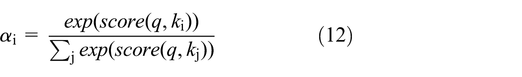
By passing the similarity score through a softmax function, it is possible to determine which inputs the model should focus on/give more importance to based on the magnitude of each score. After the normalization process, each value vector (v _i ) is multiplied by its own attention weight (α _i ) to obtain the context vector.

$$\mathrm{context}=\sum _{\mathrm{i}}{\alpha }_{\mathrm{i}}·v_{\mathrm{i}}$$

(13)

Finally, the context vector required for the model to make sense of long-term dependencies is passed through the softmax function to obtain the final output (y) of the model. This process allows the model to treat outputs from different time steps as a single vector.

$$y=\mathrm{softmax}(\mathrm{context})$$

(14)

Encoder-Decoder

Encoder-Decoder structure, first proposed in Cho et al. ²⁹ for statistical machine translation, consists of two main components, the Encoder and the Decoder, as the name suggests. The output of the Encoder, which converts the input sequence into a fixed-length context vector, serves as input for the Decoder, which is used to generate the output sequence. The encoder part is used to capture long-term dependencies in time series data, as in this study. This process is typically performed by neural networks capable of processing time series data, such as Gated Recurrent Units (GRUs) or Long-Short Term Memory (LSTMs), allowing these neural networks to act as encoders. First, a new hidden state (h _t ) is created using the current time step data point (x _t ) and the previous hidden state (h _{t −1}).

$$h_{\mathrm{t}}=f(x_{\mathrm{t}},h_{\mathrm{t}-1})$$

(15)

In this step, a fixed-size vector containing context information that summarizes long-term dependencies is generated using information from past time steps. The decoder part calculates a new hidden state (s _t ) using the previous output (y _{t −1}), the previous hidden state (s _{t −1}) and the context vector (c) generated by the encoder and thus predicts future data points.

$$s_{\mathrm{t}}=f(y_{\mathrm{t}-1},s_{\mathrm{t}-1},c)$$

(16)

Then, the decoder function (g) uses this new hidden state and context vector to produce the output of the model (y _t ).

$$y_{\mathrm{t}}=g(s_{\mathrm{t}},c)$$

(17)

In summary, the encoder part compresses data from past time steps into a fixed-size vector, while the decoder part uses this vector to predict future time steps. The Encoder-Decoder structure is widely used and successful in time series analysis, such as weather forecasting, financial data analysis, or energy load estimation, as in this study. Encoder-Decoder mechanisms can process input and output sequences of varying lengths, providing both single and probabilistic predictions. However, the original Encoder-Decoder structure’s requirement to fit the entire input sequence into a fixed-length vector can result in information loss for long sequences. To circumvent this, Encoder-Decoder structure can be hybridized with Attention mechanisms, as in the model proposed in this paper.

Fuzzy information granulation

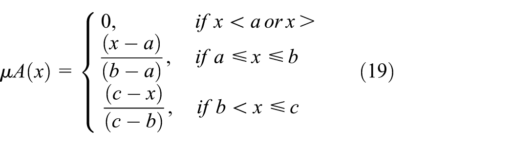
Fuzzy Information Granulation (FIG) was first used in Zadeh ³¹ to extract structured information from imprecise data. This allows large and complex datasets to be divided into meaningful pieces or granular elements, making them more manageable. The FIG method is inspired by and parallels the human thinking process; for example, humans perceive the world in granular ways, such as hot, cold, and warm. Therefore, it is logical to choose this method when working with uncertain and noisy data. In the FIG method, data are represented by fuzzy sets with a membership degree between 0 and 1. The degree to which a data item belongs to a fuzzy set, that is, its membership degree, is calculated using a membership function. Membership functions vary depending on the purpose and the dataset, such as triangular, trapezoidal, Gaussian, and bell-shaped. For example, a fuzzy set A is defined by the membership function µ _A .

$$\mu A(x):X\to [0,1]$$

(18)

In this study, the triangular membership function, frequently preferred due to its simple structure and ease of calculation, is used. This function uses the following parameters: a (the left boundary) representing the minimum value, b (the triangle vertex) representing the maximum membership value, and c (the right boundary) representing the maximum value. This allows for modeling uncertainty and simplifying the data without over-partitioning the data.

$$\mu A\left(x\right)=\{\begin{array}{c}0,\mathrm{if}x<a\mathrm{or}x>\hfill \\ \multicolumn{1}{c}{\frac{(x-a)}{(b-a)},\mathrm{if}a\le x\le b}\\ \multicolumn{1}{c}{\frac{(c-x)}{(c-b)},\mathrm{if}b<x\le c}\end{array}$$

(19)

The FIG method consists of the following stages: first, the granulation phase, where data is divided into small, meaningful pieces, then, the modeling of each resulting granule with a membership function, and finally, the granule evaluation phase, where the granules are used for data analysis and decision-making. This method allows for the piecemeal evaluation of complex patterns in large or uncertain data, leading to increased performance and lower costs. The proposed model utilizes the FIG method to enhance the relevance of long-sequence data analysis on Türkiye’s real hourly data.

Bayesian optimization

Bayesian optimization, first implemented in Jones et al. ³² to demonstrate its advantages in optimizing complex models with minimal evaluation steps and to reduce cost, is frequently preferred in the deep learning field to find optimal hyperparameters for high-cost and time-consuming functions. Compared to classical methods like grid search or random search, the Bayesian optimization method approaches the optimum with fewer trials, significantly reducing computational time and cost in a deep learning model that takes hours to train. Furthermore, this optimization method takes uncertainty into account, not only searching for the best estimate but also trying to determine which regions are worth exploring. In this study, as shown in Table 2, it was used in the hyperparameter optimization of the deep learning models used and in the granulation window size selection stages during the fuzzy information granulation phase the parameter ranges for which the most efficient choices are determined using Bayesian optimization are given in Table 2.

Table 2.

Hyperparameter ranges.

Hyperparameter	Range of considered values
Learning rate	[0.0001, 0.01]
Dropout rate	[0, 0.5]
Optimization solver	adam, sgdm, rmsprop
Number of layers	1, 2, 3
Number of neurons	[16, 64]
Number of epochs	10, 20, 30, 40
Number of timestep	3, 6, 12
Granulation window size	2, 4, 6

Bayesian optimization consists of an a priori model representing the initial belief derived from existing observations of the function and a learning function that determines the points from which new instances of the function will be selected. Gaussian Processes (GP), the most commonly used a priori model, are a powerful statistical approach that uses a covariance function (kernel) to describe the similarity between any two data points. In this study, Bayesian optimization is implemented using the GP approach.

The GP method is expressed by a mean function m(x), which models the average behaviors of the data, and a covariance function k(x, x′), which determines the similarity between two data points. In most cases, the mean function m(x) is assumed to be zero because the data are assumed to fluctuate around the general trend. This method creates a distribution that considers all possible shapes of the function and provides an estimation mechanism that accounts for uncertainty for both observed and unobserved data.

$$f~GP(m(x),k(x,x\prime ))$$

(20)

The gain function G(x) is used to select new data points by determining the most appropriate sampling point for the model. The gain function considers current estimates and the level of uncertainty. In this function, the expected value of the model at point (x) is calculated using the mean estimate (µ(x)) at that point and the standard deviation (σ(x)), which represents the uncertainty at that point, or the confidence level. The function’s (κ) value adjusts the balance between exploration and exploitation. Higher (κ) values allow the model to explore more, thus focusing on previously unexplored areas. Lower (κ) values, on the other hand, focus on exploitation, favoring areas with greater confidence and less uncertainty.

$$G(x)=\mu (x)+\kappa \sigma (x)$$

(21)

This structure allows the model to learn faster and more accurately by selecting the most efficient points. Gain functions can vary depending on the application; among the most used are Expected Recovery (EI), Probability of Recovery (PI), or Upper Confidence Bound (UCB) as chosen in this study. Furthermore, because GP has a complexity of O(n³), its scalability in very high-dimensional hyperparameter spaces is limited. To overcome this limitation, alternative methods such as Tree-structured Parzen Estimators (TPE) or Bayesian Neural Networks (BNN) have been developed, but these methods were not necessary for this study because the hyperparameter size targeted for optimization was not very large.

Data definition and preprocessing

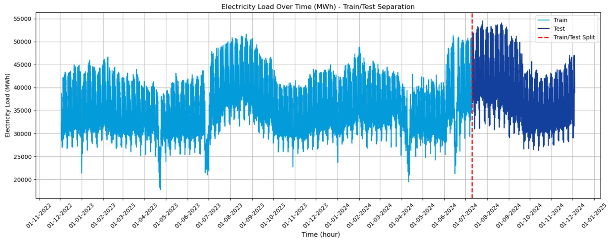
In this study, short-term electricity load forecasting is performed using Türkiye’s actual hourly electricity load data. These data consist of time-series data reflecting nationwide energy consumption, expressed in Megawatt-hours (MWh). The dataset used in this research is obtained from EPIAŞ (Energy Markets Operation Inc.). ³³ The data is collected hourly to more accurately estimate short and long-term fluctuations in energy demand. Apart from the timestamp information (year, month, and hour), no additional exogenous variables are included in the dataset, and the forecasting task is conducted using historical load values and time-related features only. The data preprocessing stage allows the model to learn data more accurately and quickly, allowing it to better cope with noise in the data, and thus improving model performance. In this study, the collected time series data was modeled as separate continuous numerical features for year, month, and hour, aiming to capture seasonal and cyclical trends. This type of decomposition within the dataset ensures more accurate future forecasts. To prevent features in the collected data from differing scales, all features were adjusted between 0 and 1 using Min-Max normalization. This allows the model to learn the data more quickly and accurately and make stable weight updates. In this study, electricity load data (MWh) was selected as the target variable for short-term forecasting.

$$X^{\prime }=\frac{(X-X_{\min })}{(X_{\max }-X_{\min })}$$

(22)

In the mathematical formula of Min-Max normalization, $X^{\prime }$ represents the scaled value, X is the original value, X_min is the minimum value of the feature, and X_max is the maximum value of the feature.

As another data preprocessing step, the fuzzy information granulation method mentioned in section “Fuzzy information granulation” was applied to the model proposed in this study to better handle the complexity and uncertainty in the collected time series data, to divide the data into fuzzy sets to treat it as more meaningful pieces of information, to obtain more consistent results in short- and long-term forecasts, and to improve the overall performance of the model.

In addition, to evaluate the performance of the model, the dataset is divided into two as 80% training (train) and 20% testing (test), as seen in the Figure 1. This process is a critical step to understand how the model performs on new and unseen data. Additionally, 10% of the training data was used as validation data to prevent overfitting during the training phase. While the training data is used to create the model’s learning process, the test data is used to evaluate the model’s generalization ability.

Figure 1.

Dataset overview.

Model integration

The dataset described above under the section “Data definition and preprocessing” consists of hourly data. This dataset, used throughout the study for electricity load estimation, requires a robust model structure to capture the complex patterns and long-term dependencies in time series. Using Türkiye’s actual hourly electricity loads may suggest that these data may be affected by environmental conditions, seasonal cycles, and economic fluctuations. To cope with such fluctuations and changes in the dataset and achieve consistent forecast results, the methods described separately in the section “Materials and methods” were employed. In this context, the model integration process is illustrated in Figure 2, following the order of the methods used. The thin green arrows highlighted in the image are intended to facilitate tracking and clearly articulate the processes implemented in this study, enhancing understanding.

Figure 2.

Overview of the proposed forecasting model.

First, the raw electric load data is converted into a granular structure using a fuzzy information granulation approach. The raw data is segmented into overlapping temporal windows with a granulation window size. The granulation window size is treated as a hyperparameter and optimized using Bayesian optimization to balance information compression and temporal resolution. For each window, three representative parameters are computed: the lower bound (minimum value), the central value (mean value), and the upper bound (maximum value). These parameters define a triangular membership function, which is used to model the local uncertainty and variability of the load values within each segment. The triangular membership function assigns a membership degree to each observation inside the window based on its relative position between the lower, mean, and upper values. Specifically, values closer to the mean receive higher membership degrees, while values approaching the minimum or maximum bounds receive lower degrees. For each time window, the minimum and maximum membership values are extracted and interpreted as the fuzzy lower and upper bounds of the granulated representation. These fuzzy bounds are then aligned temporally with the original time series and used as additional explanatory features.

Next, a deep learning-based hybrid model optimized to capture long-term dependencies in time-series data is used. In the proposed model structure, LSTM (Long Short-Term Memory) networks were chosen for the Encoder architecture due to their superior ability to preserve complex temporal patterns and long-term relationships. Meanwhile, GRU (Gated Recurrent Unit) networks were chosen for the Decoder structure due to their reduced number of parameters, resulting in computational efficiency and reducing the risk of overfitting. During sequence construction, each LSTM input sample consists of a multivariate sequence that includes the normalized load value, calendar-based temporal features (year, month, and hour), and the corresponding fuzzy granulation outputs (lower and upper membership bounds) for each time step. This structure enables the LSTM encoder to simultaneously capture raw temporal dynamics and uncertainty-aware fuzzy representations of short-term fluctuations.

The hyperparameters of the LSTM and GRU structures presented in Table 2 were optimized using the Bayesian optimization methods mentioned in section “Bayesian optimization,” and for each candidate, the values that achieved the lowest RMSE value were selected from 20 different combinations. This optimization step, performed for both deep learning architectures, strengthened the overall performance and predictive power of the proposed model.

The Encoder-Decoder structure used is enhanced by hybridizing it with an attention mechanism to learn long-term and complex dependencies in time series data. In the Encoder part, LSTM cells encode input sequences and generate hidden state vectors. These hidden vectors are passed through the attention mechanism, capturing important information, and then passed to the Decoder. The attention mechanism captures the significance and dependencies between each output value and its corresponding input vectors, thus increasing the final prediction accuracy of the model output by the Decoder.

By combining integrated short- and long-term memory, an encoder-decoder structure, and an attention mechanism, fuzzy information granulation can better capture subtle patterns in time-series data and optimize forecasting performance. Thanks to fuzzy information granulation, the uncertainty and complexity in time-series data are broken down into more manageable information granules. Then, these information granules are processed using a hybrid deep learning approach, an encoder-decoder structure, and an attention mechanism. The proposed model aims to achieve high forecasting performance, using optimized parameters in these stages. For clarity and reproducibility, the overall computational workflow of the proposed model is summarized in Appendix B, where the complete pseudo-code of the framework is provided, enabling a clear mapping between the model components and their algorithmic implementation.

Evaluation of forecasting performance

This study compares models using the most common error metrics used to evaluate model performance in time series forecasting: RMSE (Root Mean Squared Error), MAE (Mean Absolute Error), MAPE (Mean Absolute Percentage Error), and R² (R-Square). Also, U₁ (Theil’s U₁), U₂ (Theil’s U₂) statistical metrics, IA (The Index of Agreement) and P_Improvement (Percentage Improvement) metrics are also used for an innovative approach. The interpretations of these metrics are provided in this section, whereas their mathematical formulations are given in Appendix A (Table 7).

RMSE calculates the means of squared errors, then calculates the root of it, which results in penalizing large errors more. This makes RMSE more sensitive to outliers, making it a useful choice when high deviations from the true values are undesirable.

MAE averages the absolute differences between the predicted values and the actual values and provides a straightforward interpretation of how far off the model’s predictions are from the observed outcomes, regardless of direction. It can be said that MAE is more robust than RMSE because RMSE operates on the squares of the errors, meaning it is more affected by outlier values.

MAPE shows how large the percentage error in predictions is and provides an intuitive measure of forecasting accuracy by comparing the absolute difference between predicted and actual values relative to the actual value. However, it can produce unstable results in series with high variability.

R ² measures how well the model’s predictions explain the variance in the data. The closer it is to 1, the better the model’s performance. In this context, ${\hat{\mathrm{y}}}_{\mathrm{i}}$ represents the predicted value by the model, y_i is the actual observed value, $\overline{y}$ is the mean of actual values, and n is the total number of data points. A negative R² value can be obtained when the model performs even worse than the average prediction, and this is more common in short time series. It is not a sufficient metric on its own because R² does not provide information about the absolute magnitude of the errors. For example, a model that does not actually have a good predictive ability with the “copy yesterday’s value to tomorrow” method will have a very high R² value, while RMSE and MAE values will also be high.

The U₁ statistic, also known as Theil’s U₁, is a relative accuracy measure used to evaluate forecasting performance by comparing the predictive accuracy of a model against a naïve benchmark. It produces values between 0 and 1. Values of 0 and 1 represent the model’s performance between a perfect forecast (represented by 0) and a naive forecast (represented by 1). There is a linear relationship between the value close to 0 and the model’s prediction accuracy. In other words, the lower the U₁ value, the better.

Another version of Theil inequality coefficients, the U₂ statistic, is used to compare the predictive performance of a forecasting model with the performance of a naive benchmark method such as random walk. A U₂ value less than 1 indicates that the prediction model provides better prediction accuracy than the naive approach, while a U₂ value equal to 1 indicates that the model performs the same as the naive approach, and a value greater than 1 indicates that the model performs worse. It can be said that the smaller the U₂ value is at 1, the better the model performed.

The IA is a metric designed to assess the extent to which predicted values agree with actual observations. It ranges from 0 to 1, with values approaching 1 indicating high level of agreement between the predicted and observed data. In the mathematical equation presented in Table 7 (Appendix A), the value subtracted from 1 represents the normalized error rate: the numerator is the total squared error (SSE) between the predicted and observed values, and the denominator represents the maximum potential error based on deviations from the mean ( $\overline{y}$ ). A value close to 1 indicates errors close to the maximum deviation, while a value close to 0 indicates close agreement with observations. Therefore, a smaller normalized error results in a higher IA, meaning better model fit.

P _Improvement is a metric that quantifies how much better the proposed model performs in comparison to a benchmark model, based on a specific performance index such as MAE, RMSE, or MAPE. In this study, RMSE has been considered as the primary performance criterion. P_Improvement is expressed as a percentage and reflects the relative gain in predictive accuracy or error reduction, with higher values indicating greater improvement over the baseline method.

Prediction interval performance measures

In the study, the prediction intervals of the predicted values produced after the training and testing phases of the models were evaluated using the IPCP (Interval Prediction Coverage Probability) and IPAW (Interval Prediction Average Width) metrics to evaluate both the reliability and efficiency of the model.

IPCP indicates the proportion of true values that fall within the predicted interval [L _i , U _i ]. It is a key measure of interval reliability, where higher values denote better coverage. A perfect IPCP would be 1, meaning all actual values fall inside their respective intervals.

$$\mathrm{IPCP}=\frac{1}{n}\sum _{i=1}^n{c}_{i,}{c}_i=\{\begin{array}{c}1,y_{\mathrm{i}}\in [L_{\mathrm{i}},U_{\mathrm{i}}]\hfill \\ \multicolumn{1}{c}{0,y_{\mathrm{i}}\notin [L_{\mathrm{i}},U_{\mathrm{i}}]}\end{array}$$

(23)

IPAW measures the average width of the prediction intervals. Lower IPAW values indicate narrower (more confident) prediction intervals, but they must be interpreted alongside IPCP to ensure reliability is not sacrificed for sharpness. The goal is to maintain a balance between high IPCP and low IPAW for effective uncertainty quantification.

$$\mathrm{IPAW}=\frac{1}{n}\sum _{i=1}^n(U_{\mathrm{i}}-L_{\mathrm{i}})$$

(24)

Statistical hypothesis testing

The DM (Diebold-Mariano) test is a statistical hypothesis test used to compare the predictive accuracy of two competing forecasting models. Specifically, it evaluates whether the difference in forecast errors from two models is statistically significant. Let e_1,t and e_2,t denote the forecast errors from model 1 and model 2 respectively. The loss differential at time t is defined as:

$$d_{\mathrm{t}}=g(e_{1,t})-g(e_{2,t})$$

(25)

where g(·) is a loss function, such as the squared error g(e) = e².

The DM test evaluates the null hypothesis:

$$H^0:\mathbb{E}\left[d_{\mathrm{t}}\right]=0(\mathrm{no}\mathrm{difference}\mathrm{in}\mathrm{forecast}\mathrm{accuracy})$$

(26)

The test statistic is given by:

$$\mathrm{DM}=\frac{\overline{d}}{\sqrt{\frac{{\hat{\gamma }}_d(0)+2\sum _{k=1}^{h-1}{\hat{\gamma }}_d(k)}{T}}}$$

(27)

Here, $\overline{d}$ denotes the mean loss differential. The term ${\hat{\gamma }}_d(k)$ refers to the k-th order sample autocovariance of d. The parameter h represents the forecast horizon; for example, h = 1 corresponds to one-step-ahead forecasts. Lastly, T is the total number of forecasts. Under the null hypothesis, the test statistic approximately follows a standard normal distribution, that is, DM ∼ N(0, 1). A statistically significant DM statistic indicates a meaningful difference in forecast accuracy between the two models.

Results and discussion

In this section, the performance of five different models tested for the hourly estimation of the electricity load data is evaluated. For each model, 20 different hyperparameter combinations are explored using the Bayesian optimization method, and the trial with the lowest RMSE value was selected as the best performing one. As shown in Table 3, the optimal hyperparameters for each model vary significantly in terms of timestep, number of layers, neurons, learning rate, and dropout rate. Notably, the proposed FIG-LG-EDAM model was selected after 17 trials and utilized a compact granulation window size and a relatively small dropout rate, with three hidden layers and 39 neurons per layer. Despite this modest configuration, its performance surpassed all other models. The effectiveness of combining GRU with LSTM, attention mechanisms, encoder-decoder structure, and fuzzy granulation is evident in its optimized structure.

Table 3.

Selected hyperparameters.

Hyperparameters	FIG-LG-EDAM	FIG-L-EDAM	L-EDAM	L-AM	LSTM
Trial number	17	10	11	16	0
Timestep	6	12	12	5	4
Granulation size	6	6	—	—	—
Neuron number	39	63	17	34	64
Layer number	3	1	3	2	3
Dropout rate	0.007883	0.011390	0.009298	0.020938	0.042269
Learning rate	0.002464	0.000576	0.006893	0.000101	0.000853
Optimizer	Adam	Adam	Adam	Rmsprop	Adam
Epoch number	30	20	20	30	20

On the other hand, the basic LSTM model required the highest number of neurons (64) and had the highest dropout rate (0.042269), which suggests a potential attempt to counteract overfitting due to its simpler structure. Interestingly, although it converged with fewer timesteps, it delivered the weakest performance in all metrics, as detailed in Table 4.

Table 4.

Test phase results.

Metrics	FIG-LG-EDAM	FIG-L-EDAM	L-EDAM	L-AM	LSTM
RMSE	608.3382	671.5421	724.9578	872.4258	1060.7476
MAE	440.5232	493.6167	547.2091	704.3646	823.9277
R2	0.9917	0.9899	0.9883	0.9830	0.9749
MAPE	0.0113	0.0123	0.0137	0.0186	0.0200
Theil’s U1	0.0075	0.0083	0.0089	0.0107	0.0131
Theil’s U2	0.0909	0.1004	0.1083	0.1303	0.1584
IA	0.9979	0.9974	0.9970	0.9956	0.9934
IPCP	1.0000	0.9262	0.9487	0.9379	0.8924
IPAW	2036.6951	2158.7493	3344.1023	3967.8984	4089.6648

Table 4 summarizes the performance of the five forecasting models during the test phase using both point-forecast and interval-forecast evaluation metrics (bold values indicate the best results). For short-term electricity load forecasting, error-based metrics (MAE, RMSE, and MAPE) are the most directly relevant indicators of operational accuracy, as they quantify absolute and relative deviations between predicted and actual demand. In particular, RMSE is critical in this application because it penalizes large errors more strongly, which is essential for grid operation where peak-demand underestimation can lead to costly reserve and scheduling issues. In addition, reliability and stability metrics (R², IA, Theil’s U₁/U₂) and interval metrics (IPCP, IPAW) are necessary to evaluate whether a model produces not only accurate point forecasts but also useful uncertainty estimates.

In terms of point-forecast accuracy, the proposed FIG-LG-EDAM model achieves the lowest RMSE (608.3382), MAE (440.5232), and MAPE (0.0113), indicating the best overall predictive precision among all models. The performance gap becomes more pronounced when comparing structurally simpler baselines: for example, the conventional LSTM yields a substantially higher RMSE (1060.7476) and MAPE (0.0200), implying weaker generalization to unseen demand patterns. The fit quality metrics reinforce this ranking: FIG-LG-EDAM attains the highest R² (0.9917) and IA (0.9979), showing that it closely tracks the temporal variability and overall shape of the real load signal. Meanwhile, the gradual reduction in R² and IA from FIG-L-EDAM (R² = 0.9899, IA = 0.9974) to L-EDAM, L-AM, and LSTM indicates that removing components such as fuzzy granulation and attention reduces the model’s ability to represent complex, nonstationary demand dynamics.

From the perspective of relative and scale-independent performance, Theil’s U statistics provide an important robustness check. FIG-LG-EDAM produces the lowest Theil’s U₁ (0.0075) and U₂ (0.0909) values, suggesting improved predictive stability and reduced relative error compared to the benchmark models. These results imply that the proposed architecture generalizes better across varying load magnitudes and does not rely exclusively on fitting average trends.

For decision-making under uncertainty, interval forecasting metrics are particularly relevant. FIG-LG-EDAM achieves perfect coverage (IPCP = 1.0000) while maintaining the narrowest interval width (IPAW = 2036.6951), indicating an effective balance between reliability and sharpness. In contrast, the benchmark models exhibit either lower coverage or wider intervals; for instance, FIG-L-EDAM has a lower IPCP (0.9262) and a wider IPAW (2158.7493), meaning it is slightly less consistent in capturing true values within the predicted range. The conventional LSTM presents the least desirable behavior overall, with the lowest IPCP (0.8924) and the widest interval (IPAW = 4089.6648), indicating less reliable and less informative uncertainty estimation despite broader bounds.

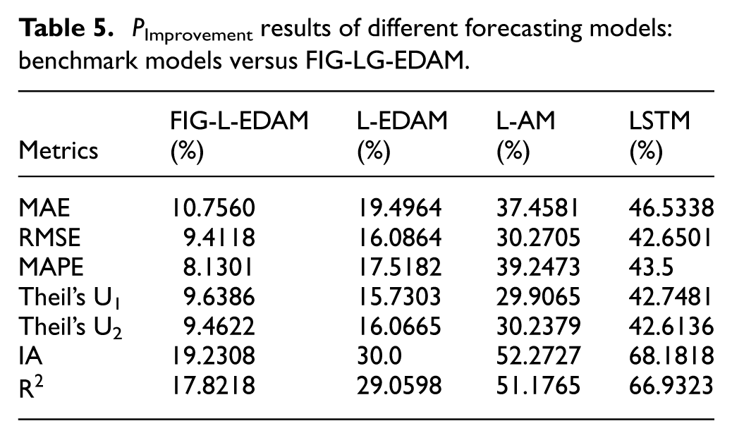
Overall, Table 4 demonstrates that the superiority of FIG-LG-EDAM is not limited to a single metric category; rather, it provides simultaneous gains in point accuracy (MAE, RMSE, MAPE), fit quality (R², IA), robustness (Theil’s U₁/U₂), and uncertainty quantification (IPCP, IPAW). These findings suggest that the proposed hybrid integration improves not only average predictive accuracy but also the practical reliability of forecasts for real-world short-term electricity load operations. These metric-specific differences are further supported by the P_Improvement analysis reported in Table 5 and the pairwise Diebold–Mariano (DM) test results presented in Table 6.

Table 5.

P _Improvement results of different forecasting models: benchmark models versus FIG-LG-EDAM.

Metrics	FIG-L-EDAM (%)	L-EDAM (%)	L-AM (%)	LSTM (%)
MAE	10.7560	19.4964	37.4581	46.5338
RMSE	9.4118	16.0864	30.2705	42.6501
MAPE	8.1301	17.5182	39.2473	43.5
Theil’s U1	9.6386	15.7303	29.9065	42.7481
Theil’s U2	9.4622	16.0665	30.2379	42.6136
IA	19.2308	30.0	52.2727	68.1818
${\mathrm{R}}^2$	17.8218	29.0598	51.1765	66.9323

Table 6.

DM test statistics and p-values.

Model names	FIG-LG-EDAM	FIG-L-EDAM	L-EDAM	L-AM	LSTM
FIG-LG-EDAM	—	−7.823 (p = 0.0000)	−10.309 (p = 0.0000)	−17.720 (p = 0.0000)	−17.184 (p = 0.0000)
FIG-L-EDAM	7.823 (p = 0.0000)	—	−1.991 (p = 0.0466)	−16.321 (p = 0.0000)	−16.458 (p = 0.0000)
L-EDAM	10.309 (p = 0.0000)	1.991 (p = 0.0466)	—	−15.137 (p = 0.0000)	−14.913 (p = 0.0000)
L-AM	17.720 (p = 0.0000)	16.321 (p = 0.0000)	15.137 (p = 0.0000)	—	−0.783 (p = 0.0437)
LSTM	17.184 (p = 0.0000)	16.458 (p = 0.0000)	14.913 (p = 0.0000)	0.783 (p = 0.0437)	—

Figures 3 to 8 illustrate the interval forecasting results of five different models evaluated on the 20% test part of Türkiye’s electricity load dataset, with each graph providing insights into the model’s ability to capture the actual load dynamics. The hourly predictions and prediction intervals are presented in 5-h increments to enhance visual interpretability. Additionally, each figure shows the results for September 27, 2024, at a magnified scale. This zoomed-in graph allows for a more detailed analysis of model performance and clearer observation of differences.

Figure 3.

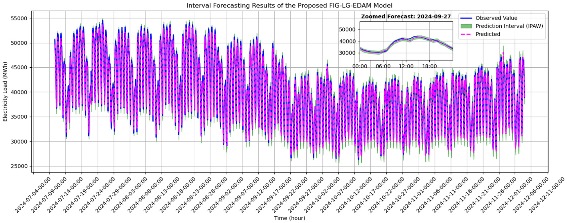
Real versus predicted values of proposed FIG-LG-EDAM model.

Figure 4.

Real versus predicted values of proposed FIG-L-EDAM model.

Figure 5.

Real versus predicted values of proposed L-EDAM model.

Figure 6.

Real versus predicted values of proposed L-AM model.

Figure 7.

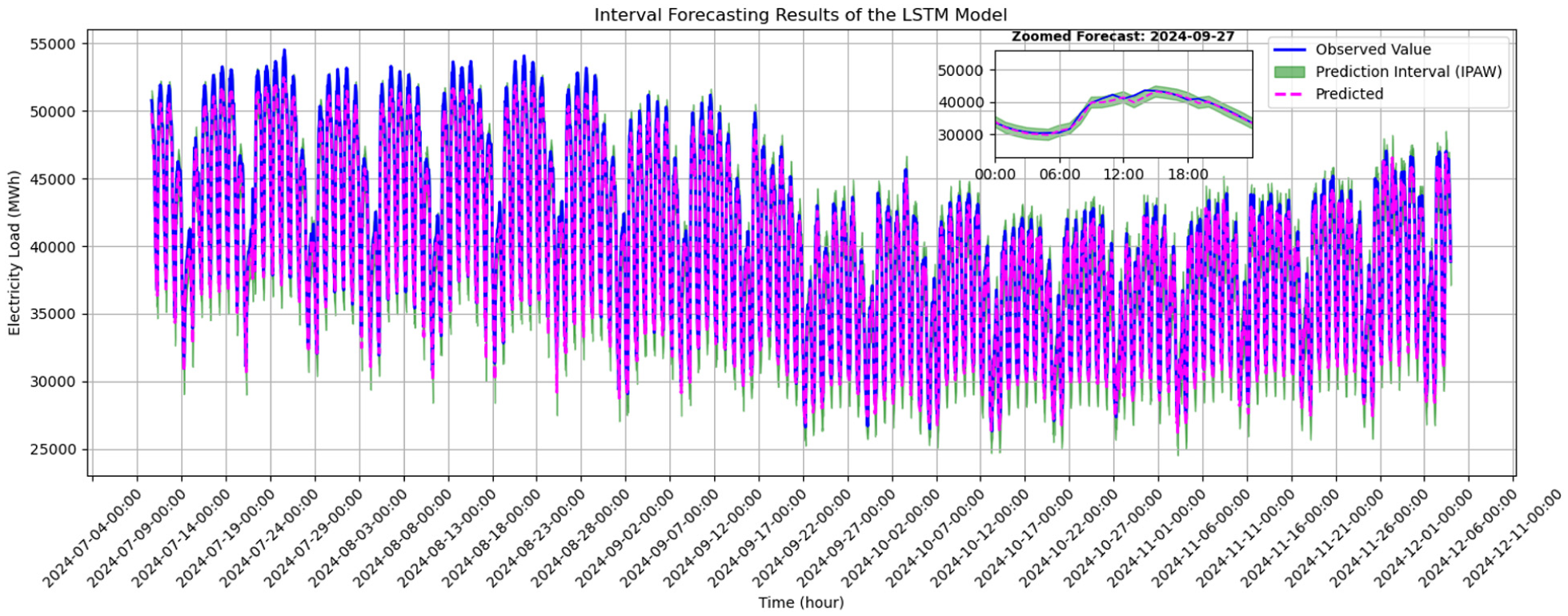
Real versus predicted values of proposed LSTM model.

Figure 8.

Real versus predicted electricity load over last 7 days.

In Figure 3, the performance of the proposed FIG-LG-EDAM model is demonstrated. It is evident that the predicted values closely follow the actual data with high fidelity. Moreover, the prediction intervals are both narrow and stable over time, indicating a robust and confident forecasting capability. The consistency between observed and predicted values, even during sudden peaks and drops in load, confirms the effectiveness of the proposed hybrid structure in handling complex time-series patterns.

Figure 4 displays the interval forecasting outcomes of the FIG-L-EDAM model. Although this model provides a good approximation to the real values and maintains relatively narrow prediction intervals, minor deviations in certain peak regions suggest that excluding the GRU integration found in the proposed model may slightly reduce temporal representation capacity.

In Figure 5, the interval forecasting results of the L-EDAM model is shown. The absence of fuzzy granulation in this structure leads to slightly wider prediction intervals and visibly larger fluctuations in forecast accuracy, especially during high variability periods. This indicates the value of modeling that takes uncertainty into consideration in increasing interval reliability.

Figure 6 shows the performance of the L-AM model, reveals a further decrease in prediction accuracy along with the widening of prediction intervals and increasing deviations from actual values. Based on this result, it can be interpreted that the L-AM model’s ability to handle rapidly changing load variations has decreased due to the absence of encoder-decoder dynamics and fuzzy information granulation methods in the model.

Finally, Figure 7 shows the prediction performance of a classic LSTM model that has not been hybridized with any other method. This model exhibits the widest prediction range and the most significant deviation from the actual data values, especially during sudden transitions. Figure 7 clearly shows that the classic model has the weakest prediction performance compared to the hybrid models used. The increased dispersion in predicted values signals lower reliability and greater forecasting uncertainty, reaffirming the necessity of hybrid and advanced architectures for accurate electrical load prediction.

Collectively, these results demonstrate the superior performance of the proposed FIG-LG-EDAM model in both point forecasting accuracy and interval reliability. The integration of GRU components, attention mechanisms, encoder-decoder structure, and fuzzy granulation enables the model to effectively capture both linear and nonlinear temporal patterns, thereby enhancing the interpretability and precision of the forecasts. This hybrid architecture also allows for noise mitigation and the extraction of important information from long-term connections. The visuals in Figures 3 to 7 support Tables 4 and 5, allowing us to conclude that model performance decreases as the model structure simplifies.

Figure 8 visualizes the comparison between the actual and predicted hourly electricity load values over the last 7 days of the testing period for five forecasting models. To enhance the interpretability of short-term performance, a 24-h zoom-in view on November 28, 2024, is provided in the lower part of the figure. This allows for a clearer interpretation of each model’s performance during sudden changes and peaks. Furthermore, the 7-day perspective on model performance also reveals how the models adapt to weekday and weekend differences. At this stage, it can be seen that the proposed model stands out with its superior performance both during seasonal variations and sudden changes.

From the visualization, it becomes evident that the forecasting accuracy progressively deteriorates as the models deviate from the proposed FIG-LG-EDAM architecture and are simplified. The FIG-LG-EDAM model exhibits the closest alignment with the actual load curve, while more basic architectures such as LSTM and LSTM with attention display increasing divergence, particularly around peak and trough hours. This clearly highlights the importance of incorporating components such as fuzzy logic, attention mechanisms, and encoder-decoder structures to capture complex temporal dependencies in electricity load patterns more effectively.

Figure 9 presents a comparative visualization of the observed and predicted hourly electricity load profiles for three representative days selected from different seasons (Figure 9(a) for summer, Figure 9(b) for fall, and Figure 9(c) for winter) within the testing period. By explicitly evaluating model performance under distinct seasonal conditions, this analysis serves as a robustness check across multiple temporal regimes. The results indicate that the proposed FIG-LG-EDAM model consistently maintains a close alignment with the actual load curve across all seasons, effectively capturing both seasonal demand shifts and intra-day load dynamics. In particular, the prediction intervals remain well-calibrated during peak and off-peak hours, demonstrating the model’s stability under varying consumption patterns. These findings suggest that, even when trained on a single regional dataset, the proposed framework exhibits robust generalization capability across heterogeneous time periods characterized by different seasonal behaviors.

Figure 9.

Seasonal forecasting performance.

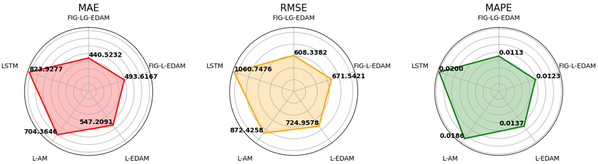
The radar charts presented in Figure 10 provide a visual overview of the comparative performance of five forecasting models across three key error metrics: Mean Absolute Error (MAE), Root Mean Square Error (RMSE), and Mean Absolute Percentage Error (MAPE). This allows for a quick comparison of performance across different metrics, making it easier to identify the models’ strengths. Each chart illustrates how individual models fare relative to one another in terms of predictive precision, where smaller values indicate better performance.

Figure 10.

Radar chart of metrics.

Across all three metrics, the FIG-LG-EDAM model consistently achieves the lowest error scores. Specifically, it records the lowest MAE (440.5232), RMSE (608.3382), and MAPE (0.0113), thereby occupying the innermost and most favorable region of each radar chart. This consistent performance underlines the model’s capability in minimizing both absolute and percentage-based forecast errors. The second-best performance is achieved by the model labeled FIG-L-EDAM, which also integrates fuzzy granulation but without the GRU layer. While its scores are slightly higher than FIG-LG-EDAM, the marginal differences suggest that fuzzy processing is a critical contributor to improved accuracy. On the contrary, the standard LSTM and its variants without fuzzy or encoder-decoder enhancements occupy the outermost regions in all charts, indicating relatively inferior performance. For instance, LSTM yields the highest MAE (823.9277), RMSE (1060.7476), and MAPE (0.0186), which implies substantial limitations in capturing temporal dependencies and noise.

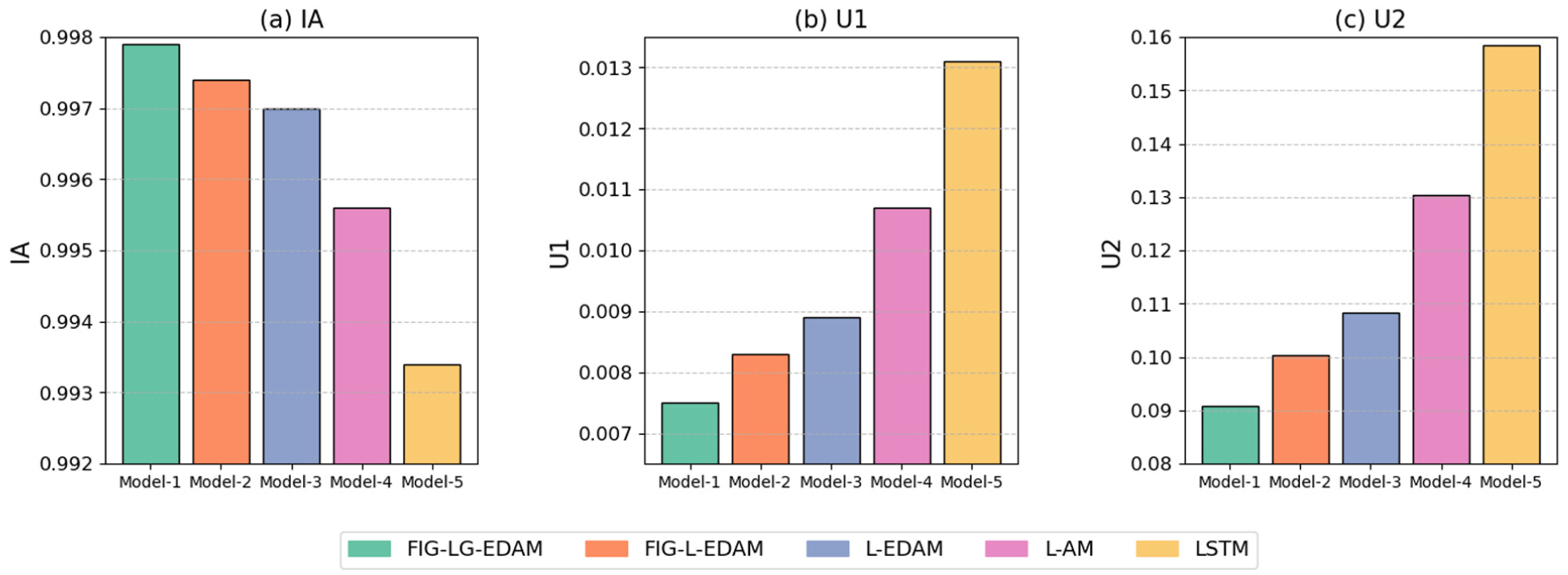
Overall, these visualizations reinforce the quantitative results shown in tabular comparisons, clearly demonstrating that the progressive incorporation of architectural elements particularly fuzzy logic and attention mechanism systematically enhances model accuracy. Figure 11 presents a comparative analysis of the five forecasting models using three performance metrics: the Index of Agreement (IA), Theil’s U₁, and Theil’s U₂. These indicators offer complementary insights into model accuracy and predictive efficiency.

Figure 11.

Performance metrics comparison.

As seen Figure 11(a), the FIG-LG-EDAM model achieves the highest IA value, closely followed by the other models enhanced with fuzzy processing and attention mechanisms. The IA metric, which ranges between 0 and 1, indicates how well the predicted values agree with the actual values. The FIG-LG-EDAM model’s superior IA value signifies its outstanding performance in capturing the true dynamics of the time series. In real-world data with varying variability, such as electricity load forecasting, adaptability to different conditions and comprehensiveness play a crucial role, as does forecast accuracy. In Figure 11(b), Theil’s U₁ statistic illustrates that the FIG-LG-EDAM model again leads with the lowest value, indicating the least deviation from the actual observations. This result reflects the model’s robustness in short-term prediction scenarios. As expected, models without fuzzy logic or encoder-decoder structure, particularly the baseline LSTM, exhibit significantly higher U₁ values. Figure 11(c) reinforces these findings with U₂ scores, where lower values suggest a better forecasting capability compared to a naïve model. Once again, the FIG-LG-EDAM model secures the best position with the smallest U₂, confirming its ability to outperform both basic and moderately complex alternatives. The standard LSTM model ranks lowest, with a substantial gap in performance.

These observations collectively emphasize the importance of incorporating advanced architectural elements-especially fuzzy information granulation, attention, and hybrid recurrent units-for enhancing both the agreement with observed data and the relative predictive power of forecasting models. In this context, the FIG-LG-EDAM model, distinguished by its superior comprehensiveness and adaptability as well as its predictive ability, has proven its potential to achieve high success on more diverse datasets.

Table 5 demonstrates the forecasting performance of four benchmark deep learning models, which are evaluated against the proposed FIG-LG-EDAM model. Each benchmark incorporates subsets of the architectural components used in FIG-LG-EDAM to assess the contribution of these elements individually and in combination, with the corresponding P_Improvement values representing the percentage performance gains computed according to the mathematical equation in the Table 7 (Appendix A).

The FIG-L-EDAM model is identified as the most competitive benchmark model, as higher P_Improvement rates are observed for all remaining baseline models when compared against the proposed FIG-LG-EDAM, indicating larger performance gaps. As shown in Table 5, the relatively lower improvement percentages observed between FIG-LG-EDAM and FIG-L-EDAM indicate that FIG-L-EDAM already incorporates several critical architectural components, including fuzzy information granulation, LSTM-based encoder–decoder structure, and an attention mechanism, making it the strongest baseline among the compared models. In contrast, substantially higher P_Improvement values are observed for models with progressively reduced architectural complexity, such as L-EDAM, L-AM, and the conventional LSTM model. This trend highlights the cumulative contribution of each architectural component to forecasting performance. In particular, the inclusion of fuzzy information granulation enables uncertainty-aware representation of load dynamics, while the encoder–decoder structure facilitates effective sequence-to-sequence learning. Furthermore, the asymmetric integration of LSTM in the encoder and GRU in the decoder in the proposed FIG-LG-EDAM model enhances long-term dependency modeling while maintaining computational efficiency. The attention mechanism further amplifies these gains by allowing the model to selectively focus on informative temporal segments, leading to consistent improvements across both error-based metrics (MAE, RMSE, and MAPE) and stability-oriented metrics (Theil’s U₁, Theil’s U₂, IA, and R²). Overall, the results demonstrate that the superior performance of FIG-LG-EDAM is not solely due to architectural depth, but rather to the synergistic interaction of fuzzy granulation, memory structures, encoder–decoder learning, and attention-based feature weighting.

Table 6 shows the Diebold–Mariano (DM) test statistics and corresponding p-values for pairwise comparisons between proposed FIG-LG-EDAM model and several benchmark alternatives used in the study. The DM test evaluates whether there is a significant difference in the estimation accuracy of two models, which allows for a clearer understanding of the performance differences between the proposed model and other benchmark models.

The p-value estimates the success rate of the more successful model among the compared models, providing insight into the reliability of the DM test results. A small p-value indicates that the probability of an extreme result, such as the predictions of two different models being completely identical, is unlikely to appear by coincidence. In this study, threshold values of p < 0.05 (significant) and p < 0.01 (very significant) were considered. The fact that p-values are below 0.01 in almost all pairwise comparisons strongly supports the existence of statistically significant differences in prediction accuracy. Positive DM statistics (upper triangle part) indicate that the row model performs better, while negative values (lower triangle part) indicate that the column model performs better.

The proposed FIG-LG-EDAM model consistently achieves the best prediction accuracy compared to all other benchmark models with a p-value of 0.0000. The FIG-L-EDAM model also significantly outperforms simpler baseline models (e.g. when compared to L-AM and LSTM, p = 0.0000). On the other hand, the superiority of the FIG-L-EDAM model over the L-EDAM model (DM = 1.991, p = 0.0466) can be interpreted as the FIG structure offers enhancement, but most of the improvements stem from the encoder-decoder structure and attention mechanism. Additionally, L-EDAM demonstrates significantly better performance than L-AM and classical LSTM models (p = 0.0000), supporting the importance of the encoder-decoder structure and attention mechanism in modeling complex temporal dependencies.

Through DM tests and p-value calculations, strong statistical evidence has been obtained that the proposed FIG-LG-EDAM model is the best-performing architecture, followed by the FIG-L-EDAM and L-EDAM models. This reflects the strong synergy between fuzzy granulation and encoder-decoder structures, and LSTM and GRU for time series predictions. The L-AM model showed a small but significant advantage over the classic LSTM architecture at the 5% level (p = 0.0437), while both were clearly disadvantaged compared to variants that included an encoder-decoder structure. As a result, the DM test not only demonstrates the high predictive success of the proposed model but also demonstrates this success through a statistical comparison with other models used. Furthermore, the generally low p-values in the Table 6 clearly demonstrate that the success of the proposed model is not random and that the used architectural components significantly impact model performance. In line with these results, it has been deemed more appropriate to prefer carefully enriched complex architectures with enhanced ability to cope with sudden changes and uncertainties instead of classical LSTM in time series studies requiring high accuracy, such as load prediction in real-world data.

Conclusion

In this study, a novel hybrid model named FIG-LG-EDAM—integrating Fuzzy Information Granulation (FIG), Long Short-Term Memory (LSTM), Gated Recurrent Unit (GRU), Attention Mechanism, and an Encoder-Decoder structure—was proposed to enhance short-term electricity load forecasting accuracy. The model’s forecasting performance is evaluated using a wide range of performance metrics using time series data representing Türkiye’s real hourly electricity load and statistically compared with different benchmark models. Various visual and numerical comparisons suggest that the proposed model outperforms other models and can be useful for forecasting similar real-world data in the energy sector.

The preferred hyperparameter combinations in this proposed hybrid model architecture are determined using the Bayesian optimization method to ensure that the model achieves its maximum performance. Despite requiring fewer neurons and epochs, the FIG-LG-EDAM model demonstrated significantly better results than benchmark models, highlighting both its training efficiency and its architectural robustness.

Beyond combining existing components, the main novelty of the proposed FIG-LG-EDAM model lies in the functional integration and role-specific interaction between fuzzy information granulation and the encoder–decoder attention-based deep learning architecture. Unlike conventional hybrid models where fuzzy preprocessing and deep learning components are loosely coupled, fuzzy granulation in FIG-LG-EDAM is embedded directly into the sequence construction stage and treated as an uncertainty-aware temporal feature rather than a standalone preprocessing step. This design allows the encoder to jointly learn raw load dynamics and fuzzy-derived uncertainty patterns at each timestep.

Furthermore, the asymmetric use of LSTM in the encoder and GRU in the decoder is intentionally designed to balance long-term dependency preservation and computational efficiency. The attention mechanism operates on fuzzy-enhanced latent representations, enabling the decoder to selectively focus on informative temporal segments where uncertainty and variability are most pronounced. This coordinated interaction between granulation, memory structures, and attention distinguishes the proposed model from existing architectures and explains its superior predictive accuracy, robustness, and interval forecasting reliability observed in the experimental results.

FIG-LG-EDAM demonstrated its ability to cope with hourly electricity demand variability by achieving the lowest MAE, RMSE, and MAPE values and the highest ${\mathrm{R}}^2$ and IA results compared to other models during the training and testing phases, demonstrating its ability to significantly outperform other models. This model, which is being considered for deployment, provides stable forecasts with minimal IPAW and reliability with maximum IPCP, thus achieving the optimal result. The superiority of the proposed model over other benchmark models is also statistically supported through pairwise DM test comparisons.

In future studies, the proposed model can be dynamically fed with new data to enhance its ability to handle real-time data. Thus, by providing active learning, improved success can be achieved in electricity load data that can show frequent and sudden changes due to seasonal and environmental factors, as in the real world. This can help the model achieve robust performance even during economic fluctuations or atmospheric events, enhancing its interpretive capacity. Additionally, to facilitate the model’s use on larger datasets, a multi-objective optimization approach that optimizes computational time as well as predictive accuracy can be considered. Similarly, efficient attention mechanism approaches, such as Longformer or Linformer, can be utilized to enhance performance on longer sequences of data.