Sage Journals: Discover world-class research

Abstract

Smart grids have recently attracted increasing attention because of their reliability, flexibility, sustainability, and efficiency. A typical smart grid consists of diverse components such as smart meters, energy management systems, energy storage systems, and renewable energy resources. In particular, to make an effective energy management strategy for the energy management system, accurate load forecasting is necessary. Recently, artificial neural network–based load forecasting models with good performance have been proposed. For accurate load forecasting, it is critical to determine effective hyperparameters of neural networks, which is a complex and time-consuming task. Among these parameters, the type of activation function and the number of hidden layers are critical in the performance of neural networks. In this study, we construct diverse artificial neural network–based building electric energy consumption forecasting models using different combinations of the two hyperparameters and compare their performance. Experimental results indicate that neural networks with scaled exponential linear units and five hidden layers exhibit better performance, on average than other forecasting models.

Keywords

Short-term load forecasting building energy consumption forecasting artificial neural network hyperparameter tuning scaled exponential linear unit

Introduction

Smart grids, which are known to have features including reliability, flexibility, sustainability, and efficiency, have emerged as a solution for numerous current problems, including energy shortage and environmental pollution.^1–3 A smart grid is a platform for exchanging real-time power information supported by wired/wireless communication, control, and sensors between suppliers and consumers to enable innovative power management.^1,2 Typical smart grids comprise smart meters, energy management systems (EMSs), energy storage systems (ESSs), and diverse renewable energy resources. In particular, an EMS determines ways to save energy on the demand side by collecting and analyzing data related to building energy consumption within an electric power system.³ On the supply side, an EMS generates schedules for power generation and ESSs by considering a number of factors, including storage costs and the amount of energy to be used in the future.⁴ In order to generate more effective schedules, an EMS requires accurate short-term load forecasting (STLF).^5,6

The aim of STLF is to ensure the reliability of the electric power system equipment and prepare for losses caused by power failures and overloading by controlling electricity reserve margins.^7–9 STLF is typically used to predict the electric load on an hourly basis up to 1 week in advance for daily operation and cost minimization.^10,11 For instance, accurate STLF can provide economic benefits by storing energy at night when electric costs are relatively low and emitting electricity during the day when electric costs are high.⁹ STLF includes daily peak electric load, total daily electric load, hourly electric load, and very short-term load forecasting (VSTLF; e.g., 15-min and 30-min interval load forecasting).¹²

STLF is not an easy task because energy consumption patterns are complex, and uncertain external factors can cause a shift in the demand curve.^13,14 Factors affecting the fluctuation in building electric energy consumption include architectural structure, thermal properties of physical materials, time zones, electricity rates, special events, resident schedules, climatic conditions, and lighting.^14,15 In addition, when forecasting electric loads, complex energy consumption correlations between the current time and the previous time should be appropriately considered.^16,17 To date, numerous artificial neural network (ANN)–based STLF models have been constructed to predict exact electric loads and have exhibited favorable performance.^18–35 To further improve their performance, it is critical to effectively tune their hyperparameters. All ANN models have various hyperparameters (i.e. the number of hidden layers (HLs), number of hidden nodes, activation functions, number of epochs, learning rate, batch size, optimizers, loss function, and so on) to specify the structure of the network itself or to determine how to train neural networks (NN).^36,37 Of these, the two most essential hyperparameters are the activation function and the number of HLs.³⁷

Activation functions assist the network in separating useful data from noise^38–41 and are also used to introduce nonlinearity to models, which allows ANN models to learn nonlinear prediction boundaries. As their forecasting results are highly dependent on the activation function, selecting a proper activation function is critical for improving forecasting performance. Increasing the number of HLs does not always improve forecasting accuracy.^42,43 In addition, a too-large increase in the number of HLs can decrease accuracy in the test set because of overfitting the training set.⁴² In other words, when the ANN model with too many HLs learns the training data, it is difficult to generalize to new unseen data.⁴³

Although these hyperparameters are critical in the performance of ANN models, no studies have compared the prediction performance by considering various activation functions and number of HLs for STLF. Therefore, in this study, we construct an ANN-based STLF model for forecasting electric energy consumption of building or building clusters accurately. In order to apply our STLF model for other building or building clusters, we consider general factors such as calendar data, weather information, and historical electric loads and perform data preprocessing using them. Then, we perform extensive experiments to compare the performance of various activation functions and number of HLs for selecting an optimal ANN-based STLF model.

The primary contributions of this study can be summarized as follows.

For day-ahead energy scheduling in a smart grid, we build an ANN-based STLF model with a focus on electric energy consumption of a building or building clusters.

We consider general factors such as calendar data, weather information, and historical electric loads to apply our STLF model as the baseline model for other building or building clusters.

We predict the 30-min interval electric load for five different types of buildings by setting several cases as test sets.

We extensively compare overall prediction performances of activation functions and the number of HLs for constructing an optimal ANN-based STLF model.

The rest of this article is organized as follows. In section “Related studies,” we review related studies on STLF. In section “Data collection and preprocessing,” we describe the data preprocessing procedures that transform the historical load data and external information to input vectors of the ANN-based model. In section “ANN-based energy forecasting modeling,” we demonstrate the 30-min interval electric load forecasting model based on ANNs. In section “Experimental results,” we describe the experimental design and present the experimental results. Finally, in section “Conclusion,” we conclude the results and proposed future study directions.

Related studies

In this section, we review a number of STLF studies (including those on VSTLF) that have been conducted for the efficient operation of smart grid systems. To date, several ANN-based electric load forecasting models have been developed. Table 1 presents the STLF-related studies based on ANN.

Table 1.

Summary of short-term load forecasting based on ANNs.

Reference	Granularity	Input variables	NN	Number of hidden layers	Activation function
Park et al.¹⁸	1 h	Calendar data, weather condition	FFNN, RNN, NARX network	1	tanh
Mordjaoui et al.¹⁹	30 min	Calendar data, historical load	Dynamic NN	1	No mention
Qiu et al.²⁰	30 min	Economic factors, calendar data, weather condition, random effects	RVFL network	1	Logistic sigmoid
Reddy²¹	1 h	Historical load, weather condition	BPNN	1	Sigmoid
Hu et al.²²	1 h	Historical load, weather condition	GRNN	1	No mention
Ertugrul²³	15 min	Calendar data, weather condition, historical load	ELM	1	Sigmoid
Zeng et al.²⁴	1 h	Calendar data, weather condition, historical load	ELM	1	tanh
Li et al.²⁵	1 h	Calendar data, weather condition, historical load	ELM	1	Sigmoid
Mocanu et al.²⁶	1 min	Historical load	RBM	1	Sigmoid
Raza et al.²⁷	1 h	Calendar data, weather condition, historical load	LM-based NN	1	No mention
Elgarhy et al.²⁸	1 h	Calendar data, historical load	LM-based NN	1	Logistic sigmoid
Singh et al.²⁹	1 h	Calendar data, weather condition, historical load	BPNN	1	Sigmoid
Dedinec et al.³⁰	1 h	Calendar data, weather condition, historical load, cheap tariff flag	DBN	2	tanh
Qiu et al.³¹	30 min	Economic factors, calendar data, weather condition, random effects	DBN	2	No mention
Ryu et al.³²	1 h	Calendar data, weather condition, historical load	DBN, DNN	4	DBN: sigmoid, DNN: ReLU
Fan et al.³³	1 h	Calendar data, weather condition, chilled water temperature	DAE, DNN	DAE: 3, DNN: 2	DAE: tanh,DNN: ReLU
Din and Marnerides³⁴	1 h	Calendar data, weather condition, historical load	FFNN, RNN	FFNN: no mentionRNN: 1	FFNN: ReLU
Kuo and Huang³⁵	1 h	Historical load	CNN	3	ReLU

ANN: artificial neural network; NN: neural networks; FFNN: feedforward neural network; RNN: recurrent neural networks; NARX: nonlinear autoregressive exogenous; RVFL: random vector function link; BPNN: backpropagation neural networks; GRNN: generalized regression neural networks; ELM: extreme learning machine; RBM: restricted Boltzmann machine; LM: Levenberg–Marquardt; DBN: deep belief networks; DNN: deep neural network; DAE: deep auto-encoder; CNN: convolutional neural network; ReLU: rectified linear units.

Park et al.¹⁸ compared three NN-based electric load forecasting models: feedforward neural network (FFNN), recurrent neural network (RNN), and neural network-based nonlinear autoregressive exogenous (NARX) models. The forecasting results indicated that the NN-based NARX model is superior to the other models because it can reuse the predicted load data for reflecting the forecast trend. Mordjaoui et al.¹⁹ proposed a dynamic NN-based electric load forecasting model and compared it to the Holt–Winters exponential smoothing (ES) and seasonal autoregressive integrated moving average (SARIMA) models. They reported that their model could achieve better mean absolute percentage error (MAPE). Qiu et al.²⁰ proposed an STLF model based on empirical mode decomposition (EMD) and a random vector function link (RVFL) network. They used EMD to decompose the electric load data into a number of intrinsic mode functions and one residue. The RVFL network was then trained for each intrinsic mode function, including the residue. They reported that their model performed best of six benchmarking models (i.e. Persistence, support vector regression (SVR), single-HL feedforward NN, RVFL, EMD, and EMD-based SVR). Reddy²¹ proposed a Bat algorithm-based backpropagation approach for forecasting short-term electric loads considering weather factors (i.e. temperature and humidity). Their approach significantly reduced the trial and error effort in the training phase and also produced an STLF technique that was more efficient, adaptive, and optimized than the ANN-based approaches. Hu et al.²² proposed an STLF model based on a generalized regression neural network (GRNN) and reported that the prediction accuracy of the model was higher than that of the backpropagation neural network (BPNN). Ertugrul²³ reported a 15-min interval electric load forecasting model based on recurrent extreme learning machine (RELM). In RELM, extreme learning machine (ELM) was adapted to train a single hidden-layer Jordan RNN. The RELM exhibited better performance than other machine learning methods, such as traditional ELM, linear regression, and GRNN, in terms of root mean square error (RMSE). Zeng et al.²⁴ proposed a hybrid hourly electric load forecasting model based on ELM and switching delayed particle swarm optimization (SDPSO) methods. In the model, input weights and ELM biases were optimized by the SDPSO method. The model significantly improved the forecasting accuracy compared to the radial basis function NN. Li et al.²⁵ proposed an ensemble hourly STLF model based on wavelet transform, ELM, and partial least squares regression (PLSR). Their wavelet-based ensemble approach employed different wavelet specifications to create an ensemble of individual predictors. For each subcomponent obtained from the wavelet decomposition, a parallel forecasting model of 24 ELMs was established. To improve the accuracy of the model, individual outputs were combined using the PLSR method. They reported that their model could provide superior forecasting accuracy compared with other forecasting models. Mocanu et al.²⁶ suggested two STLF models based on the conditional restricted Boltzmann machine (CRBM) and factored conditional restricted Boltzmann machine (FCRBM). In terms of forecasting accuracy, FCRBM outperformed ANN, SVR, RNN, and CRBM. Raza et al.²⁷ compared the ability of backpropagation and Levenberg–Marquardt (LM) training method of ANN for STLF. They considered historical electric load, time factors, and weather information as an input variable of the ANN-based STLF model. They used their forecasting models to predict the hourly electric load of the ISO New England grid. Their experimental results indicate that LM showed better results than the backpropagation in terms of MAPE. Elgarhy et al.²⁸ proposed an hourly electric load forecasting model based on LM-based ANN. They applied to multiple datasets and the results obtained were compared to the published results. Singh et al.²⁹ presented hourly electric load forecasting model of New England Power Pool (NEPOOL) at ISO New England using LM-based ANN. They used historical electric load, time factors, and weather information as input variables and hourly electric load as output variable to train ANN. Separate training and forecasting have been done for working days, weekends only, and weekends including holidays. Since the ISO New England dataset used in previous studies^27–29 has extensive geographical coverage of the collected electric load, it showed uncomplicated electric energy consumption patterns. Therefore, ANN with one HL showed satisfactory prediction performance by training simple patterns adequately. However, our goal is to predict the electric energy consumption of buildings or building clusters that exhibits complex energy consumption patterns. Hence, we consider not only ANN with one HL but also a deep neural network (DNN) with two or more HLs to reflect the complex energy consumption patterns effectively.

A DNN was recently used in electric load forecasting.^44–46 For instance, Dedinec et al.³⁰ proposed an STLF model using deep belief networks (DBN), which comprised multiple layers of restricted Boltzmann machine (RBM). The forecasting results of the DBN were compared with those of the FFNN and the forecasting load data provided by the Macedonian system operator. The MAPE of the proposed model was higher than the other forecasting models. Qiu et al.³¹ reported an ensemble deep learning method based on EMD and DBN for STLF. They compared nine benchmark methods (i.e. Persistence, SVR, ANN, DBN, random forest, ensemble DBN, EMD-based SVR, EMD-based single-HL feedforward NN, and EMD-based random forest) to verify the effectiveness of their proposed method. They evaluated the prediction performance of forecasting models using RMSE and MAPE. Their EMD-based ensemble deep learning approach exhibited superior performance in statistical testing. Ryu et al.³² proposed two DNN-based load forecasting models using pre-training RBM and rectified linear units (ReLU) without pre-training. The forecasting results indicated that their models were more accurate and robust compared to other forecasting methods, such as shallow NN, double seasonal Holt-Winters, and SARIMA. Fan et al.³³ developed deep learning-based methods for achieving accurate and reliable day-ahead building cooling load forecasting. The deep learning-based methods (DNN; supervised learning, deep auto-encoder (DAE); unsupervised learning) were compared to seven benchmark methods (supervised learning) and existing feature extraction methods (unsupervised learning), used in the building field, in terms of accuracy and computation efficiency. The results indicated that deep learning-based methods could enhance the prediction performance, particularly when the DAE was used to construct high-level features as forecasting model inputs. Din and Marnerides³⁴ built two STLF models based on feedforward deep NNs and recurrent DNNs and reported that they enabled the extraction of a feature from the original “raw” power measurements by exploiting the joint time–frequency representation of the load signals. Their method could model the most dominant factors that affected the electric load patterns. Kuo and Huang³⁵ proposed a deep convolutional neural network (CNN)-based STLF model, in which the input layer denoted information of previous electric loads, and the output values represented the forecast electric load. They reported that the most critical feature could be extracted by the designed one-dimensional (1D) convolution and pooling layers and that their model was more accurate than five artificial intelligence methods, including SVR, random forest, decision tree, multilayer perceptron (MLP), and long short-term memory (LSTM) network.

In addition, the LSTM-based RNN exhibited favorable performance in real-time STLF.^2,44–46 However, the LSTM networks could reflect the previous point for the forecasting of the next point.¹⁰ As the day-ahead building electric energy consumption forecasting of a smart grid should be scheduled until after 1 day, LSTM networks are not suitable for 30-min interval electric load forecasting because there is a gap of 47 points. Therefore, we focus on the ANN-based electric load forecasting model for efficient day-ahead scheduling in smart grids.

Data collection and preprocessing

In this study, we use electronic Watt-hour meter data collected from the Korea Electric Power Corporation (KEPCO) for five different building types in South Korea. Table 2 presents the data collection periods and information about the buildings. Data were collected every 30 min.

Table 2.

Building information.

Type	Description	Data collection period (days)	Number of buildings
A	Office building	2015-01-01–2016-12-31 (731)	1
B	Factory building	2015-01-01–2016-12-31 (731)	1
C	Education building (lecture)	2015-01-01–2016-12-31 (731)	32
D	Education building (laboratory)	2015-01-01–2016-12-31 (731)	19
E	Education building (dormitory)	2015-01-01–2016-12-31 (731)	16

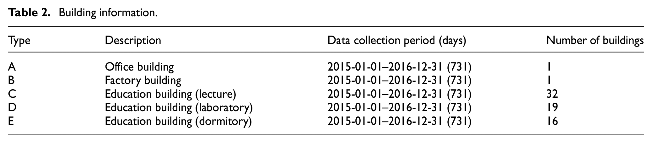
The building electric energy consumption patterns show different characteristics depending on building types. For instance, a university campus shows high electric energy consumption during the office hour, class hour, and special events.⁴⁷ However, if these factors are reflected in the forecasting model, it is challenging to utilize for typical building electric energy consumption forecasting model because it cannot be applied to other buildings and building types. Hence, we used 120 input variables comprising calendar data, weather information, and historical electric load to construct the typical ANN-based STLF model. These factors can be easily collected and applied to other buildings and building types. More detailed explanations for the selection of input variables are given in the next section.

Calendar data

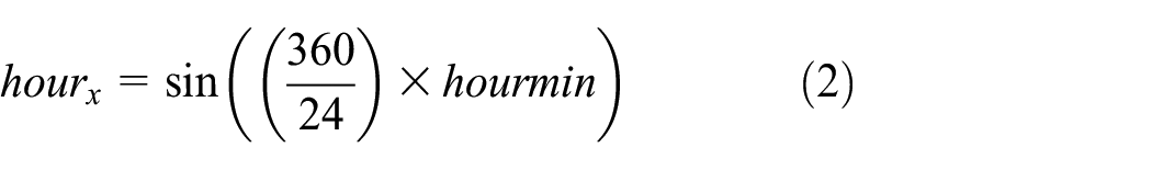
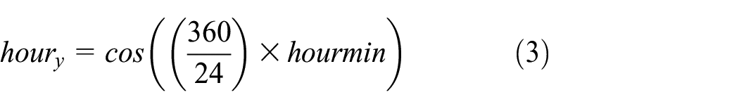
As time series data represent trends in electric loads, we consider all input variables that could express calendar data: month, day, hours to minutes, days of the week, and holidays, as presented in Table 3. In particular, as the month, day, hour, and minute have periodic properties, they were not represented by sequential values. For instance, although 11 p.m. and midnight are adjacent, their sequence difference in the sequence format is 23. In addition, although 31 March and 1 April are adjacent, their difference is 31 in the sequence format. To reflect such period properties, we transform time data using equations (1)–(7). These equations enhance the sequence data in 1D space to continuous data in two-dimensional (2D) space.⁴⁷

hourmin = hour + (\frac{minute}{60})

(1)

hou r_{x} = \sin ((\frac{360}{24}) \times hourmin)

(2)

hou r_{y} = \cos ((\frac{360}{24}) \times hourmin)

(3)

da y_{x} = \sin ((\frac{360}{Eo M_{month}}) \times day)

(4)

da y_{y} = \cos ((\frac{360}{Eo M_{month}}) \times day)

(5)

mont h_{x} = \sin ((\frac{360}{12}) \times month)

(6)

mont h_{y} = \cos ((\frac{360}{12}) \times month)

(7)

Table 3.

Calendar data input variables.

Number	Input variable	Type of variable
1	Hour_x	Continuous on [–1, 1]
2	Hour_y	Continuous on [–1, 1]
3	Day_x	Continuous on [–1, 1]
4	Day_y	Continuous on [–1, 1]
5	Month_x	Continuous on [–1, 1]
6	Month_y	Continuous on [–1, 1]
7	Monday	Binary
8	Tuesday	Binary
9	Wednesday	Binary
10	Thursday	Binary
11	Friday	Binary
12	Saturday	Binary
13	Sunday	Binary
14	Holiday	Binary

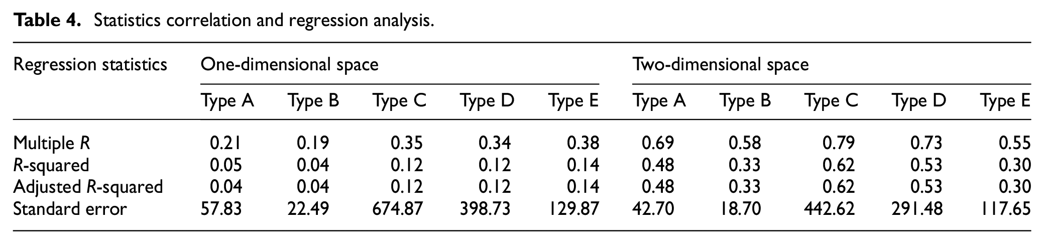
In the case of minutes, there are only two cases (0, 30). Therefore, the hour and minutes can be reflected in the corresponding time as shown in equation (1) and then applied to equations (2) and (3). Figure 1 shows hour information in 2D space using equations (2) and (3). Using this representation, we can make 11:30 p.m. and 12:00 a.m. adjacent, which is similar to the clock shape. Similarly, we can represent the day and month data in 1D space to continuous data in 2D space using equations (4)–(5) and (6)–(7), respectively. To verify the validity and applicability of 2D representation, we calculated several regression statistics on the electric loads in 1D space (month, day, hour, and minute) and in 2D space as shown in Table 4. In the table, we can see that 2D representation can explain their correlation more effectively than 1D representation. Therefore, equations (2)–(7) give a total of six input variables to represent the date and time of the prediction time points.

Figure 1.

Two-dimensional representation of a day based on 30-min interval.

Table 4.

Statistics correlation and regression analysis.

Regression statistics	One-dimensional space					Two-dimensional space
Regression statistics	Type A	Type B	Type C	Type D	Type E	Type A	Type B	Type C	Type D	Type E
Multiple R	0.21	0.19	0.35	0.34	0.38	0.69	0.58	0.79	0.73	0.55
R-squared	0.05	0.04	0.12	0.12	0.14	0.48	0.33	0.62	0.53	0.30
Adjusted R-squared	0.04	0.04	0.12	0.12	0.14	0.48	0.33	0.62	0.53	0.30
Standard error	57.83	22.49	674.87	398.73	129.87	42.70	18.70	442.62	291.48	117.65

The bulk of buildings or building clusters have electric load patterns by days of the week according to the building type.^6,10 For instance, hotels and retail premises, such as department stores and shopping malls, exhibit similar electric load patterns on weekdays and weekends. However, typical office buildings and industrial buildings have significant energy consumption on weekdays and low energy consumption on weekends. In South Korea, electric loads and energy consumption are typically low on national public holidays, such as the Lunar New Year holiday and Korean Thanksgiving days, called Chuseok.^10,17 Therefore, various electric load patterns can be observed according to weekdays and holidays. To reflect these factors, days of the week and holidays should be considered in the forecasting models. In this context, holidays include Saturdays, Sundays, and national public holidays. We collected the holiday information in South Korea at Time and Date (https://www.timeanddate.com/holidays/) that can confirm national public holidays information in many countries. Therefore, we define an 8D feature vector of 0 or 1, comprising 7 days of the week and holidays.

Weather information

The use of products with high-energy consumption, such as heating, ventilation, and air conditioning systems, is closely related to weather conditions.^8,48 Therefore, input variables derived from weather information are commonly used for STLF in numerous studies.⁴⁹ The Korea Meteorological Administration (KMA) provides various weather forecasting information, which include temperature, humidity, wind speed, daily maximum temperature, daily minimum temperature, and amount of precipitation data for every region in South Korea as shown in Figure 2.⁵⁰

Figure 2.

Example of weather forecasting by KMA.

We use the aforementioned weather variables in this study. However, since the weather forecasting information is collected at 3-h resolution unlike electric load data, it is difficult to apply the forecasting model directly. In order to make the same time resolution of energy consumption, the weather forecasting information is estimated at 30-min resolution using linear interpolation. In particular, to establish a more direct association with energy consumption, we calculate the discomfort index (DI)⁵¹ and wind chill (WC)⁵² with equations (8) and (9), respectively. Then, we use these calculated values as input variables

\begin{matrix} DI = (1.8 \times T + 32) \\ - [(0.55 - 0.0055 \times H) \times (1.8 \times T - 26)] \end{matrix}

(8)

\begin{matrix} WC = 13.12 + 0.06215 \times T - 11.37 \times W S^{0.16} \\ + 0.3965 \times T \times W S^{0.16} \end{matrix}

(9)

where T and H are the temperature and the humidity, respectively, and WS is the wind speed. Hence, we use eight weather variables (i.e. temperature, humidity, wind speed, daily maximum temperature, daily minimum temperature, amount of precipitation, DI, and WC) for building STLF models.

Historical electric load

Electric load forecasting models aim to forecast day-ahead electric loads. In addition to the 24 input variables described earlier, we also use recent historical electric loads as input variables to reflect recent trends in energy consumption. To predict one point in the day later, we consider a total of 98 input variables as the 30-min electric load data and holiday information of the previous 2 days.¹⁶ Figure 3 shows an example of historical electric loads of Type A as input variables. For instance, if the forecast time is 4:00 p.m. 4 January, we then use 96 historical load data (2 measurements/h × 24 h/day × 2 days) from 4:30 p.m. 1 January to 4:00 p.m. 3 January and two-holiday information (same point of previous 1 and 2 days) from 2 January to 3 January.

Figure 3.

Example of historical electric load as input variables.

As mentioned earlier, we consider 120 input variables; however, they have different scales. For smoothing the imperfection of ANN training, normalization is required to place all inputs within a comparable range. Therefore, we performed minimum–maximum normalization to all input variables¹⁶ as follows

z_{i} = \frac{x_{i} - \min (x)}{\max (x) - \min (x)}

(10)

ANN-based energy forecasting modeling

An ANN, which is also known as an MLP, is a type of machine learning algorithm that is an FFNN architecture with an input layer, one or more HLs, and an output layer.⁵³ Each layer comprises a number of nodes. Each node receives values from nodes on the previous layer, determines its output, and passes it to nodes on the next layer. As this process is repeated, the nodes of the output layer provide the desired values. Figure 4 shows a typical ANN structure for STLF.

Figure 4.

ANN structure for short-term load forecasting.

The HL has numerous factors that affect the performance of the network, including the number of layers and nodes and the activation function of the nodes. Therefore, the performance of the network is dependent on how the HLs are configured. In particular, the number of HLs determines the depth or shallowness of the network. For instance, when the number of HLs is two or more, the network is a so-called DNN.^32,33 Typically, an increase in the number of HLs is known to improve network performance. However, the increase could cause problems such as overfitting on the training data or difficult generalization on the new data.⁴³ In this case, the accuracy of the prediction decreases. Therefore, it is essential to determine the correct number of HLs to solve the given problem.

A sigmoid function has been an excellent activation function in NNs. However, it has a significant disadvantage, the so-called vanishing gradient problem.³⁴ The values of a sigmoid function fall within the range [0, 1] and, because of its nature, small and large values passed through the function will become close to zero and one, respectively. This means that its gradient will be close to zero and learning will be slow. As ReLU was proposed as an activation function to solve the vanishing gradient problem,³⁸ numerous other activation functions have been proposed including LReLU, PReLU, ELU, and SELU, which will have described in more detail in the following section.

Activation function

In numerous studies on the ANN-based STLF, the most fundamental ANN structure had one HL, and sigmoid functions were typically used.^{21,23,25,26,29} However, DNNs have been consistently adopted in numerous real-world applications because of their high predictive power,^38,41 and ReLU has been used when the number of HLs was two or more.^32–35 However, using ReLUs can cause the following two problems: it can result in deactivated neurons and the learning can be slow. To solve these problems, diverse activation functions have been introduced, including LReLU, PReLU, ELU, and SELU. There are numerous cases of performance comparisons of activation functions in several fields. However, there are insufficient cases in the field of STLF, and to consider all the data is time-consuming. We consider five activation functions shown in Figure 5, which have been used before for constructing STLF models.

Figure 5.

Plots of five activation functions.

ReLU

This is one of the most popular activation functions because it can solve the vanishing gradient and overfitting problems.^38,40 Therefore, it allows for effective training of ANN architecture and can be defined as follows

f (x) = {\begin{matrix} 0 \\ x \end{matrix} \begin{matrix} for x < 0 \\ for x \geq 0 \end{matrix}

(11)

Leaky rectified linear unit

Leaky rectified linear unit (LReLU) allows a small, non-zero gradient when the unit is not active.³⁸ If ReLU is used as the activation function, a number of neurons might not be activated, which could lead to poor results. By using a non-zero gradient, we can alleviate this type of problem and improve the training speed. LReLU can be defined as follows

f (x) = {\begin{matrix} 0.2 x \\ x \end{matrix} \begin{matrix} for x < 0 \\ for x \geq 0 \end{matrix}

(12)

Parametric rectified linear unit

The parametric rectified linear unit (PReLU) is inspired by LReLU. It increases the learning speed by not deactivating a number of neurons.³⁹ Compared to LReLU, PReLU substitutes the non-zero gradient values by a parameter α, as shown in the following equation

f (α, x) = {\begin{matrix} α x \\ x \end{matrix} \begin{matrix} for x < 0 \\ for x \geq 0 \end{matrix}

(13)

Exponential linear unit

The exponential linear unit (ELU) is another type of activation function based on ReLU. As in other rectified units, ELU speeds up the learning and alleviates the vanishing gradient problem.⁴⁰ As the shape of the function is smooth, the learning speed is faster than when the neuron is deactivated or has a non-smooth slope. The equation for the ELU is as follows

f (α, x) = {\begin{matrix} α (e^{x} - 1) \\ x \end{matrix} \begin{matrix} for x < 0 \\ for x \geq 0 \end{matrix}

(14)

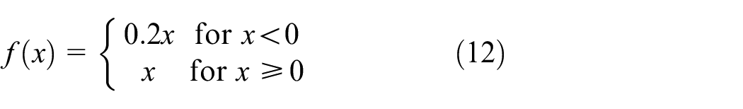
Scaled exponential linear unit

The scaled exponential linear unit (SELU) activation function is a type of ELU that uses two parameters. Learning by using two parameters improves the performance of a model because the variance of the activation function is constant.⁴¹ As SELU also has a smooth slope, its learning is fast. The equation for the SELU is as follows

f (α, λ, x) = {\begin{matrix} λ (α e^{x} - α) \\ λ x \end{matrix} \begin{matrix} for x < 0 \\ for x \geq 0 \end{matrix}

(15)

where, α, which is about 1.67326, is a stochastic variable sampled from a uniform distribution at training time and fixed to the expectation value of the distribution at test time. λ is an extra parameter involved, which is about 1.0507.

Other hyperparameters tunings

We construct ANN-based load forecasting models using all possible combinations of HLs from 1 to 10 together with activation functions. We consider five activation functions, including ReLU, LReLU, PReLU, ELU, and SELU. From the studies by Heaton⁵³ and Sheela and Deepa,⁵⁴ the number of hidden neurons should be 2/3 the size of the input layer, plus the size of the output layer. Therefore, we use 81 nodes for our forecasting model. In addition, we used Xavier initialization^55,56 to sort initial weights for individual inputs in a neuron model. When constructing an ANN model, two important hyperparameters are the learning rate and learning epoch.⁵⁷ Learning rate indicates how much the weights of the network are adjusted with respect to the loss gradient.^37,57 If the learning rate is too large, the average loss will increase.⁵⁴ Conversely, if the learning rate is too small, it might take a long time to converge the performance goal due to more exploration in the parameter space.⁵² Learning epoch indicates the period that the network learns all training data once.³² As the number of epochs increases, the weights are changed accordingly in the NN and the learning curve goes from underfitting to optimal and eventually to overfitting.⁵⁷ However, since the network is overly focused on the training data, it could show low performance for unseen data. As with the learning rate, increasing the number of epochs requires a longer time to converge the performance goal. To construct more accurate learning model, we used a learning rate of 0.000001 and learning epoch of 10,000 based on our previous experiences with these hyperparameters.⁵⁸ In addition, we set the batch size to 144 and used the RMSProp optimizer⁵⁹ and Huber loss function, which is less sensitive to outliers than the mean square error (MSE) loss function.⁵⁶

Experimental results

Data description

For the experiments, we performed preprocessing for the dataset in the Python environment and performed forecast modeling using TensorFlow.⁶⁰ Table 5 presents the statistics of the building electric energy consumption data. The electric load data were collected from 1 January 2015 to 31 December 2016. In order to obtain sufficient prediction results for each forecasting model, we set the ratio of the dataset to the training (in-sample) and test (out-of-sample) sets at approximately 50:50. Among them, we used electric load data from 1 January 2015 to 3 January 2015 to configure input variables for a training set. The data from 4 January 2015 to 3 January 2016 were used as a training set, and 4 January 2016 to 31 December 2016 were used as a test set.

Table 5.

Statistics of building energy consumption data.

Item	Building type
Item	A	B	C	D	E
Number of valid cases	35,088	35,088	35,088	35,088	35,088
Mean	101.76	20.53	1321.31	1223.62	563.82
Standard deviation	59.17	22.90	719.72	423.94	140.37
Median	79.44	8.59	1123.68	1067.04	543.96
Trimmed mean	90.98	15.68	1248.84	1165.15	554.34
Median absolute deviation	37.72	5.97	777.83	338.74	142.51
Minimum	42.81	3.79	221.93	686.40	232.56
Maximum	358.32	147.46	3424.80	2650.08	1039.32
Range	315.51	143.67	3202.87	1963.68	806.76
Skew	1.74	1.91	0.67	1.03	0.58
Kurtosis	3.06	3.57	−0.71	0.17	−0.15
Standard error	0.32	0.12	3.84	2.26	0.75

Performance measurement

To compare the performance of forecasting models, we used a coefficient of variation of the root mean square error (CVRMSE) and MAPE, which are easier to understand than other performance metrics such as RMSE or MSE because they represent accuracy as a percentage of the error. However, it is known that CVRMSE and MAPE increase significantly when the actual value tends to zero.¹⁰ The CVRMSE and MAPE equations are shown in equations (16) and (17), respectively, where $n$ is the number of times observed, $\bar{Y}$ is an average of the actual values, and $Y_{i}$ and ${\hat{Y}}_{i}$ are the actual and predicted values, respectively

CVRMSE = \frac{100}{\bar{Y}} \sqrt{\frac{\sum_{i = 1}^{n} {(Y_{i} - {\hat{Y}}_{i})}^{2}}{n}}

(16)

MAPE = \frac{100}{n} \sum_{i = 1}^{n} | \frac{Y_{i} - {\hat{Y}}_{i}}{Y_{i}} |

(17)

Comparison of activation functions

Tables 6 –10 present the forecasting results when different numbers of HLs and activation functions for five building types are used. It can be seen that building type B exhibits poor prediction accuracy compared to the other building types. This is because its electric loads are close to zero. In order to confirm the overall prediction performance of the activation functions, we present the averaged accuracy of the activation functions for different building types with the best accuracy in bold. A cooler color (blue) indicates a lower CVRMSE/MAPE value, while a warmer color (red) indicates a higher CVRMSE/MAPE value for each activation function in building types. As can be seen in the tables, ANN models with one HL generally have poor predictive performance.

Table 6.

Comparison of CVRMSE and MAPE for building type A.

Number of HLs	CVRMSE					MAPE
Number of HLs	ReLU	LReLU	PReLU	ELU	SELU	ReLU	LReLU	PReLU	ELU	SELU
1	20.57	24.36	21.10	22.38	23.02	12.59	16.16	13.07	12.90	13.66
2	18.46	19.19	18.25	19.61	19.09	10.85	11.02	10.77	11.33	10.79
3	17.67	18.03	17.32	18.34	17.14	10.10	10.54	10.24	10.81	10.04
4	16.70	18.05	17.84	18.05	16.52	10.16	10.83	10.39	10.43	10.24
5	16.74	16.91	16.72	16.97	15.67	10.73	10.15	10.57	10.56	9.76
6	17.19	16.89	16.85	17.48	16.72	10.15	10.46	9.98	10.53	10.01
7	16.48	16.55	16.03	17.62	16.23	10.33	10.02	10.07	11.52	10.38
8	16.99	17.72	17.47	17.52	14.97	10.52	11.12	10.37	11.60	10.31
9	17.22	17.39	16.54	17.27	16.67	10.72	10.29	10.11	11.76	11.00
10	16.42	16.65	17.21	17.93	17.31	10.30	11.14	10.50	12.01	11.53
Average	17.44	18.17	17.53	18.32	17.34	10.65	11.17	10.61	11.35	10.77

CVRMSE: coefficient of variation of the root mean square error; MAPE: mean absolute percentage error; HL: hidden layer; ELU: exponential linear unit; SELU: scaled exponential linear unit; ReLU: rectified linear units; LReLU: leaky rectified linear unit; PReLU: parametric rectified linear unit.

Bolded values represent the best values.

Table 7.

Comparison of CVRMSE and MAPE for building type B.

Number of HLs	CVRMSE					MAPE
Number of HLs	ReLU	LReLU	PReLU	ELU	SELU	ReLU	LReLU	PReLU	ELU	SELU
1	52.23	53.01	52.30	53.23	52.98	30.47	30.51	29.38	30.04	29.96
2	51.52	52.36	51.19	53.25	52.49	29.25	29.33	27.78	30.23	29.15
3	50.48	52.62	52.11	51.34	50.65	27.15	28.81	28.17	29.06	28.06
4	51.46	50.89	51.31	51.41	49.06	26.95	27.89	27.70	29.74	28.18
5	51.71	51.59	49.79	51.99	48.59	28.09	27.87	27.09	28.82	26.28
6	50.58	50.45	50.29	51.83	48.11	26.31	28.49	27.26	29.98	28.18
7	51.16	50.45	50.01	52.19	49.66	27.12	26.27	27.45	28.60	28.25
8	50.64	50.27	50.85	50.67	49.91	26.88	26.13	27.27	29.53	28.28
9	49.29	48.81	49.71	48.80	47.77	27.34	26.43	27.50	27.98	27.83
10	51.50	50.89	51.58	48.91	49.40	28.03	28.05	28.22	28.02	31.39
Average	51.06	51.13	50.91	51.36	49.86	27.76	27.98	27.78	29.20	28.56

Bolded values represent the best values.

Table 8.

Comparison of CVRMSE and MAPE for building type C.

Number of HLs	CVRMSE					MAPE
Number of HLs	ReLU	LReLU	PReLU	ELU	SELU	ReLU	LReLU	PReLU	ELU	SELU
1	13.32	13.50	12.66	13.61	13.35	9.38	9.69	8.70	10.38	10.14
2	12.32	12.09	12.36	12.40	11.72	8.44	8.46	8.53	8.60	8.30
3	12.37	11.97	12.20	12.00	11.62	8.28	8.25	8.23	8.37	7.89
4	11.87	12.11	12.11	11.94	11.74	8.09	8.24	8.42	8.40	7.97
5	11.76	11.93	11.90	12.08	11.31	7.97	7.97	8.03	8.39	7.98
6	12.10	11.79	12.17	11.56	11.51	8.15	8.18	8.07	8.01	7.68
7	12.03	11.94	12.11	11.53	11.47	8.13	7.94	8.19	8.05	8.04
8	11.63	11.64	12.13	11.45	11.66	7.95	7.89	8.15	7.92	8.08
9	11.81	11.64	11.85	11.67	10.71	7.87	8.09	8.17	8.20	7.30
10	12.19	11.65	11.77	11.60	11.83	8.02	8.13	7.99	8.53	8.36
Average	12.14	12.03	12.13	11.98	11.69	8.23	8.28	8.25	8.48	8.17

Bolded values represent the best values.

Table 9.

Comparison of CVRMSE and MAPE for building type D.

Number of HLs	CVRMSE					MAPE
Number of HLs	ReLU	LReLU	PReLU	ELU	SELU	ReLU	LReLU	PReLU	ELU	SELU
1	10.34	9.66	9.01	10.04	9.69	7.48	6.88	6.16	7.26	6.98
2	8.75	8.23	8.35	8.47	8.13	6.10	5.65	5.71	5.83	5.58
3	8.27	8.18	8.49	8.46	8.14	5.66	5.54	5.70	5.87	5.51
4	8.23	8.25	8.13	8.41	7.82	5.58	5.58	5.48	5.88	5.32
5	8.12	8.01	8.23	8.34	7.76	5.52	5.41	5.59	5.73	5.31
6	8.08	8.09	8.00	8.08	7.81	5.47	5.44	5.38	5.54	5.28
7	7.98	8.08	8.26	8.19	7.58	5.33	5.47	5.37	5.58	5.17
8	8.55	8.11	8.19	7.98	7.81	5.66	5.54	5.43	5.44	5.26
9	8.33	7.90	8.08	8.09	7.61	5.54	5.30	5.39	5.51	5.26
10	7.99	7.87	8.28	8.04	7.35	5.29	5.37	5.42	5.44	5.11
Average	8.46	8.24	8.30	8.41	7.97	5.76	5.62	5.56	5.81	5.48

CVRMSE: coefficient of variation of the root mean square error; MAPE: mean absolute percentage error; HL: hidden layer; ELU: Exponential linear unit; SELU: scaled exponential linear unit; ReLU: rectified linear units; LReLU: leaky rectified linear unit; PReLU: parametric rectified linear unit.

Bolded values represent the best values.

Table 10.

Comparison of CVRMSE and MAPE for building type E.

Number of HLs	CVRMSE					MAPE
Number of HLs	ReLU	LReLU	PReLU	ELU	SELU	ReLU	LReLU	PReLU	ELU	SELU
1	8.74	9.05	8.52	9.37	8.98	6.57	6.82	6.38	7.17	6.84
2	8.08	8.08	8.29	8.14	7.92	6.09	6.19	6.27	6.14	5.99
3	7.98	8.10	8.12	8.14	7.87	6.07	6.17	6.15	6.14	6.00
4	7.98	7.81	8.21	7.73	7.75	6.06	5.94	6.29	5.91	5.88
5	8.02	7.87	8.17	8.03	7.89	6.12	5.99	6.18	6.09	6.02
6	8.02	7.71	7.69	7.91	7.82	6.08	5.92	5.88	6.03	6.00
7	7.96	7.95	7.93	7.92	8.08	6.07	6.02	6.03	6.08	6.17
8	7.78	8.01	8.12	7.91	7.95	5.91	6.14	6.20	6.06	6.05
9	7.92	7.83	7.91	8.03	8.22	6.05	5.97	6.06	6.16	6.30
10	8.12	8.10	7.75	7.92	7.83	6.23	6.19	5.96	6.04	5.96
Average	8.06	8.05	8.07	8.11	8.03	6.12	6.13	6.14	6.18	6.12

Bolded values represent the best values.

Tables 11 and 12 present the averaged CVRMSE and MAPE results of the activation functions and rank of activation functions for different building types. It can be seen that SELU and ELU exhibit the best and worst performances in bulk of the cases, respectively. ANN models with SELU repeatedly exhibit a higher frequency than other activation functions. Herein, we provide reasoning on why the ANN models with SELU show better prediction performance as follows.⁴¹

Compared with ReLU, SELU solves the problem of off-state as zero gradients by passing negative values to the next layer. This enables SELU to train deep NNs effectively because there is no vanishing gradient problem.

Unlike LReLU and PReLU, the shape of SELU function shows a continuous curve when x < 0 by using an exponential function. Due to this function, a gradient can get close to 0, which can shift the mean of each layer’s output values to 0. Since this enables SELU to have a superior self-normalization quality, SELU can be trained faster and better than other activation functions that are combined with batch normalization.

SELU is an activation function that multiplies ELU by λ > 1 to ensure the gradient greater than 1. To adjust the variance of each layer’s output values effectively, two regions are required: one with a gradient larger than 1 and the other with a gradient close to zero. Since SELU function satisfies these two conditions by multiplying ELU by λ, it shows better performance than ELU.

Table 11.

Average CVRMSE and rank of activation functions (the best in bold).

Activation function	Average CVRMSE					Rank of activation functions
Activation function	Type A	Type B	Type C	Type D	Type E	Type A	Type B	Type C	Type D	Type E	Average
ReLU	17.44	51.06	12.14	8.46	8.06	2	3	5	5	3	3.6
LReLU	18.17	51.13	12.03	8.24	8.05	4	4	3	2	2	3.0
PReLU	17.53	50.91	12.13	8.30	8.07	3	2	4	3	4	3.2
ELU	18.32	51.36	11.98	8.41	8.11	5	5	2	4	5	4.2
SELU	17.34	49.86	11.69	7.97	8.03	1	1	1	1	1	1.0

CVRMSE: coefficient of variation of the root mean square error; ELU: exponential linear unit; SELU: scaled exponential linear unit; ReLU: rectified linear units; LReLU: leaky rectified linear unit; PReLU: parametric rectified linear unit

Table 12.

Average MAPE and rank of activation functions (the best in bold).

Activation function	Average MAPE					Rank of activation functions
Activation function	Type A	Type B	Type C	Type D	Type E	Type A	Type B	Type C	Type D	Type E	Average
ReLU	10.65	27.76	8.23	5.76	6.12	2	1	2	4	2	2.2
LReLU	11.17	27.98	8.28	5.62	6.13	4	3	4	3	3	3.4
PReLU	10.61	27.78	8.25	5.56	6.14	1	2	3	2	4	2.4
ELU	11.35	29.20	8.48	5.81	6.18	5	5	5	5	5	5.0
SELU	10.77	28.56	8.17	5.48	6.12	3	4	1	1	1	2.0

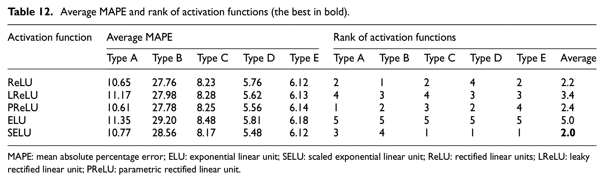
MAPE: mean absolute percentage error; ELU: exponential linear unit; SELU: scaled exponential linear unit; ReLU: rectified linear units; LReLU: leaky rectified linear unit; PReLU: parametric rectified linear unit.

Comparison of number of HLs with SELU

In the previous section, we showed the excellent performance of SELU. Therefore, in this section, we focus on the effect of the number of HLs. Tables 6 –10 show the prediction performance of all activation functions depending on the number of HLs. However, as the ranges of the performance measurement values are too diverse for each building type, it is not appropriate to calculate their average for performance comparisons. Therefore, we counted the rank of the number of HLs by building types and presented these results with CVRMSE/MAPE values of the SELU in Tables 13 and 14, respectively. A cooler color (blue) indicates a lower CVRMSE/MAPE value for each building type, while a warmer color (red) indicates a higher CVRMSE/MAPE value for each building type.

Table 13.

CVRMSE results of the number of hidden layers for SELU.

Building type	Number of hidden layers (rank)
Building type	1	2	3	4	5	6	7	8	9	10
A	23.02 (10)	19.09 (9)	17.14 (7)	16.52 (4)	15.67 (2)	16.72 (6)	16.23 (3)	14.97 (1)	16.67 (5)	17.31 (8)
B	52.98 (10)	52.49 (9)	50.65 (8)	49.06 (4)	48.59 (3)	48.11 (2)	49.66 (6)	49.91 (7)	47.77 (1)	49.40 (5)
C	13.35 (10)	11.72 (7)	11.62 (5)	11.74 (8)	11.31 (2)	11.51 (4)	11.47 (3)	11.66 (6)	10.71 (1)	11.83 (9)
D	9.69 (10)	8.13 (8)	8.14 (9)	7.82 (7)	7.76 (4)	7.81 (5)	7.58 (2)	7.81 (5)	7.61 (3)	7.35 (1)
E	8.98 (10)	7.92 (6)	7.87 (4)	7.75 (1)	7.89 (5)	7.82 (2)	8.08 (8)	7.95 (7)	8.22 (9)	7.83 (3)

CVRMSE: coefficient of variation of the root mean square error; SELU: scaled exponential linear unit.

Table 14.

MAPE results of the number of hidden layers for SELU.

Building type	Number of hidden layers (rank)
Building type	1	2	3	4	5	6	7	8	9	10
A	13.66 (10)	10.79 (7)	10.04 (3)	10.24 (4)	9.76 (1)	10.01 (2)	10.38 (6)	10.31 (5)	11.00 (8)	11.53 (9)
B	29.96 (9)	29.15 (8)	28.06 (3)	28.18 (4)	26.28 (1)	28.18 (4)	28.25 (6)	28.28 (7)	27.83 (2)	31.39 (10)
C	10.14 (10)	8.30 (8)	7.89 (3)	7.97 (4)	7.98 (5)	7.68 (2)	8.04 (6)	8.08 (7)	7.30 (1)	8.36 (9)
D	6.98 (10)	5.58 (9)	5.51 (8)	5.32 (7)	5.31 (6)	5.28 (5)	5.17 (2)	5.26 (3)	5.26 (3)	5.11 (1)
E	6.84 (10)	5.99 (3)	6.00 (4)	5.88 (1)	6.02 (6)	6.00 (4)	6.17 (8)	6.05 (7)	6.30 (9)	5.96 (2)

MAPE: mean absolute percentage error; ELU: exponential linear unit; SELU: scaled exponential linear unit

The average ranking values of all CVRMSE and MAPE values for each number of HLs are shown in Figure 6. In the figure, the SELU model with five and six HLs exhibits the lowest average ranking values of CVRMSE and MAPE, which indicate excellent prediction performance, respectively.

Figure 6.

The average ranking value of number of hidden layers for SELU.

In order to demonstrate that ANN with SELU and five HLs is the most effective, we represented average ranking values and ranking of these values, by considering CVRMSE and MAPE values for each building type as shown in Tables 15 and 16, respectively. In Table 15, a cooler color (blue) indicates a lower CVRMSE/MAPE value, while a warmer color (red) indicates a higher CVRMSE/MAPE value. Clevert et al.⁴⁰ concluded that ELU leads not only to faster learning but also to significantly better generalization performance than ReLU and LReLU on networks with more than five layers. SELU is some kind of ELU due to the constant factor α. As a result, Tables 15 and 16 show that significant values for ANN with SELU obtained on networks with more than five layers. In addition, an ANN with SELU and five HLs was found to be the best.

Table 15.

The average ranking value of CVRMSE/MAPE values for each building type when the different number of hidden layers and activation functions are used.

Number of hidden layers	CVRMSE					MAPE
Number of hidden layers	ReLU	LReLU	PReLU	ELU	SELU	ReLU	LReLU	PReLU	ELU	SELU
1	46.4	48.6	45.6	49.2	48.0	47.6	48.4	45.4	48.4	47.8
2	39.0	36.6	39.0	44.4	29.0	37.6	38.8	34.8	41.0	29.2
3	31.2	34.8	37.6	36.4	17.8	22.4	31.4	28.6	36.2	14.0
4	24.6	27.6	33.2	27.8	8.4	18.2	24.6	28.6	30.0	11.8
5	24.2	21.0	24.4	31.6	4.8	24.2	12.4	25.0	34.0	7.6
6	24.0	15.2	17.0	21.0	6.6	17.0	21.2	9.2	25.4	10.0
7	19.6	18.2	21.4	24.8	10.4	16.6	9.6	15.2	30.0	21.0
8	20.2	21.8	31.2	16.2	11.0	15.6	20.2	22.6	26.0	18.0
9	21.4	12.4	14.4	18.8	12.0	18.2	11.2	17.0	30.8	20.6
10	25.4	18.2	23.4	16.4	13.4	20.2	27.2	17.8	29.2	27.2

CVRMSE: coefficient of variation of the root mean square error; MAPE: mean absolute percentage error; ELU: Exponential linear unit; SELU: scaled exponential linear unit; ReLU: rectified linear units; LReLU: leaky rectified linear unit; PReLU: parametric rectified linear unit.

Table 16.

The average ranking value of CVRMSE/MAPE values for each building type when the different number of hidden layers and activation functions are used.

Number of hidden layers	CVRMSE					MAPE
Number of hidden layers	ReLU	LReLU	PReLU	ELU	SELU	ReLU	LReLU	PReLU	ELU	SELU
1	47	49	46	50	48	47	49	46	49	48
2	43	41	43	45	34	43	44	41	45	34
3	35	39	42	40	14	23	39	32	42	8
4	29	32	38	33	3	16	26	32	36	6
5	27	20	28	37	1	25	7	27	40	1
6	26	10	13	20	2	12	22	2	28	4
7	18	15	22	30	4	11	3	9	36	21
8	19	24	35	11	5	10	18	24	29	15
9	22	7	9	17	6	16	5	12	38	20
10	31	15	25	12	8	18	30	14	34	30

CVRMSE: coefficient of variation of the root mean square error; MAPE: mean absolute percentage error; ELU: exponential linear unit; SELU: scaled exponential linear unit; ReLU: rectified linear units; LReLU: leaky rectified linear unit; PReLU: parametric rectified linear unit.

Comparison of prediction performance via statistical techniques

To verify the validness and applicability of the ANN model with SELU and five HLs, we compare the predictive performance of the ANN model with other statistical techniques such as Persistence, moving average (MV), ES, and multiple linear regression (MLR). Persistence model assumes that the conditions at the predicted value (48-step ahead) are the same as the current values, which has good accuracy due to the highly periodic characteristic of energy consumption.^20,31 The MV method is commonly used to smooth out short-term fluctuations and highlight longer-term trends for time series data. While the MV method gives equal weights to include values, the ES method assigns exponentially decreasing weights as the observation get older, a more reasonable approach. Based on previous electric loads only at the same point, we set to 2 (interval) and 0.3 (attenuation factor) for constructing MV and ES methods, respectively.¹⁷ MLR is used to determine a mathematical relationship among a number of random variables. In other terms, MLR examines how multiple input variables are related to one output variable. We set to 120 input variables applied by ANN models for MLR model construction. We compared the prediction performance of five methods, by considering the test periods and learning model in the same environment. As shown in Table 17, the ANN model has the best prediction performance.

Table 17.

CVRMSE/MAPE values when the statistical techniques and ANN with SELU and five hidden layers are used.

Type	Methods	CVRMSE					MAPE
Type	Methods	January–March	April–June	July–September	October–December	Average	January–March	April–June	July–September	October–December	Average
A	Persistence	32.90	40.83	49.36	30.42	42.40	18.57	18.95	24.84	15.84	19.56
	MV	34.47	43.64	53.99	33.34	24.65	22.51	23.13	32.48	20.36	45.93
	ES	31.87	39.71	48.85	30.23	41.72	20.05	20.49	28.10	17.85	21.64
	MLR	19.69	27.18	34.49	19.03	28.57	19.01	21.55	25.93	18.91	21.37
	ANN	10.61	15.00	19.16	9.34	15.67	9.75	9.26	11.65	8.40	9.76
B	Persistence	79.50	81.46	84.34	92.76	87.68	60.89	52.69	55.69	47.46	54.11
	MV	81.09	86.44	91.99	95.30	91.04	77.96	69.71	79.54	57.21	71.04
	ES	75.91	79.50	83.10	91.11	85.22	69.64	61.71	68.28	52.01	62.84
	MLR	64.55	59.80	61.27	68.11	66.86	53.25	60.40	65.87	55.49	58.81
	ANN	41.56	51.18	50.69	50.25	48.59	28.85	21.81	25.59	28.92	26.28
C	Persistence	31.07	32.98	36.40	29.79	33.07	18.73	16.65	17.65	17.68	17.67
	MV	31.74	34.42	38.26	31.65	34.58	22.63	20.41	21.87	21.07	21.49
	ES	29.80	31.86	35.28	29.22	32.04	20.38	18.22	19.38	18.87	19.20
	MLR	17.42	21.00	22.74	17.94	20.15	18.12	21.44	21.62	17.84	19.77
	ANN	10.19	10.85	12.63	10.72	11.31	9.03	7.33	8.00	7.61	7.98
D	Persistence	21.39	22.62	24.89	21.81	23.01	12.03	12.08	12.13	13.22	12.37
	MV	22.61	24.36	27.13	24.70	25.07	14.97	14.86	15.73	16.80	15.60
	ES	20.84	22.16	24.57	22.26	22.78	13.21	13.06	13.54	14.79	13.66
	MLR	12.32	13.69	15.55	12.96	13.92	10.15	11.34	11.73	10.75	11.00
	ANN	6.56	7.18	8.36	8.55	7.76	5.06	4.73	5.53	5.95	5.31
E	Persistence	15.46	13.36	15.16	14.12	14.68	10.75	8.90	9.18	9.99	9.70
	MV	16.15	14.00	16.51	15.21	15.67	12.02	9.69	10.85	11.28	10.95
	ES	15.00	12.92	14.98	13.97	14.38	10.90	8.84	9.59	10.26	9.89
	MLR	9.97	9.17	10.30	9.03	9.73	8.14	7.31	7.86	7.30	7.65
	ANN	8.64	6.81	8.20	7.46	7.89	6.77	5.22	6.37	5.75	6.02

CVRMSE: coefficient of variation of the root mean square error; MAPE: mean absolute percentage error; ANN: annual neural network; SELU: scaled exponential linear unit; MV: moving average; ES: exponential smoothing; MLR: multiple linear regression.

Bolded values represent the best values.

Conclusion

In this study, we constructed diverse ANN models using different numbers of HLs and diverse activation functions and compared their performances in a 30-min STLF resolution. We considered ReLU, LReLU, PReLU, ELU, and SELU as activation functions, and the number of HLs from 1 to 10. To compare the prediction performance with two hyperparameters for the STLF model, we considered electric load data collected from five different types of buildings for 2 years, and two performance metrics, CVRMSE and MAPE. The experimental results indicated that an SELU-based model with five HLs exhibited better average performance than other ANN-based STLF models. In order to apply for every building, our proposed model is sufficient as a baseline model due to simply input variables and model configuration. In addition, our proposed model can be used to predict several time-resolution building energy consumptions in the future. For instance, if an hourly building electric energy consumption forecasting model is constructed, the input variables can be constructed by applying equations (2)–(7) in the calendar information and the rest as described earlier (14 time factors, 8 weather information, and 50 historical electric loads holiday information). Then, 49 hidden nodes can be used for constructing an SELU-based model with five HLs. Otherwise, if a 15-min interval building electric energy consumption forecasting model is constructed, the input variables can be constructed by applying equations (1)–(7) in the calendar information and the rest as described earlier (14 time factors, 8 weather information, and 194 historical electric loads holiday information). Then, 145 hidden nodes can be used for constructing an SELU-based model with five HLs.

Although we have proposed a typical building electric energy consumption forecasting model, a more accurate forecasting model can be constructed by adding new input variables that can reflect the characteristics of target building energy consumption. In addition, tuning of other hyperparameters in the SELU model can expect to improve prediction performance for the target building.

In future studies, we plan to collect additional datasets and perform experiments to investigate the robustness of our results. In addition, we will build a more sophisticated forecasting model such as multi-step ahead or probabilistic load forecasting, considering other external variables that are closely related to electric loads.

Footnotes

Handling Editor: Pascal Lorenz

Declaration of conflicting interests

The author(s) declared no potential conflicts of interest with respect to the research, authorship, and/or publication of this article.

Funding

The author(s) disclosed receipt of the following financial support for the research, authorship, and/or publication of this article: This research was supported in part by the Korea Electric Power Corporation (grant number: R18XA05) and in part by Energy Cloud R&D Program (grant number: 2019M3F2A1073184) through the National Research Foundation of Korea (NRF) funded by the Ministry of Science and ICT.

ORCID iD

Eenjun Hwang

References

Khan

Mahmood

Safdar

, et al. Load forecasting, dynamic pricing and DSM in smart grid: a review. Renew Sust Energ Rev 2016; 54: 1311–1322.

Marino

Amarasinghe

Manic

. Building energy load forecasting using deep neural networks. In: Proceedings of the IECON 2016–42nd annual conference of the IEEE industrial electronics society, Florence, 23–26 October 2016, pp.7046–7051. New York: IEEE.

Barbato

Bolchini

Geronazzo

, et al. Energy optimization and management of demand response interactions in a smart campus. Energies 2016; 9: 398.

Song

Lee

Kim

, et al. Optimal energy management of multi-microgrids with sequentially coordinated operations. Energies 2015; 8: 8371–8390.

Yue

, et al. Economic power schedule and transactive energy through an intelligent centralized energy management system for a DC residential distribution system. Energies 2017; 10: 916.

Yildiz

Bilbao

Sproul

. A review and analysis of regression and machine learning models on commercial building electricity load forecasting. Renew Sust Energ Rev 2017; 73: 1104–1122.

Ahmad

Hassan

Abdullah

, et al. A review on applications of ANN and SVM for building electrical energy consumption forecasting. Renew Sust Energ Rev 2014; 33: 102–109.

Powell

Sriprasad

Cole

, et al. Heating, cooling, and electrical load forecasting for a large-scale district energy system. Energy 2014; 74: 877–885.

Kim

Shin

Kim

. Operation strategy of multi-energy storage system for ancillary services. IEEE T Power Syst 2017; 32: 4409–4417.

10.

Moon

Kim

Son

, et al. Hybrid short-term load forecasting scheme using random forest and multilayer perceptron. Energies 2018; 11: 3283.

11.

Zheng

Yuan

Chen

. Short-term load forecasting using EMD-LSTM neural networks with a Xgboost algorithm for feature importance evaluation. Energies 2017; 10: 1168.

12.

Hong

Fan

. Probabilistic electric load forecasting: a tutorial review. Int J Forecast 2016; 32: 914–938.

13.

Mat Daut

Hassan

Abdullah

, et al. Building electrical energy consumption forecasting analysis using conventional and artificial intelligence methods: a review. Renew Sust Energ Rev 2017; 70: 1108–1118.

14.

Zhao

Magoulès

. A review on the prediction of building energy consumption. Renew Sust Energ Rev 2012; 16: 3586–3592.

15.

Jiang

. Load profile analysis and short-term building load forecast for a university campus. In: Proceedings of 2016 IEEE power and energy society general meeting (PESGM), Boston, MA, 17–21 July 2016, pp.1–5. New York: IEEE.

16.

Kwon

Park

, et al. Analysis of short-term load forecasting using artificial neural network algorithm according to normalization and selection of input data on weekdays. In: Proceedings of the 2018 IEEE PES Asia-Pacific power and energy engineering conference (APPEEC), Kota Kinabalu, Malaysia, 7–10 October 2018, pp.280–283. New York: IEEE.

17.

Moon

Kim

, et al. A short-term electric load forecasting scheme using 2-stage predictive analytics. In: Proceedings of the IEEE international conference on big data and smart computing (BigComp), Shanghai, China, 15–17 January 2018, pp.219–226. New York: IEEE.

18.

Park

Lee

Son

, et al. A comparison of neural network-based methods for load forecasting with selected input candidates. In: Proceedings of the 2017 IEEE international conference on industrial technology (ICIT), Toronto, ON, Canada, 22–25 March 2017, pp.1100–1105. New York: IEEE.

19.

Mordjaoui

Haddad

Medoued

, et al. Electric load forecasting by using dynamic neural network. Int J Hydrogen Energ 2017; 42: 17655–17663.

20.

Qiu

Suganthan

Amaratunga

. Electricity load demand time series forecasting with empirical mode decomposition based random vector functional link network. In: Proceedings of the 2016 IEEE international conference on systems, man, and cybernetics (SMC), Budapest, Hungary, 9–12 October 2016, pp.001394–001399. New York: IEEE.

21.

Reddy

. Bat algorithm-based back propagation approach for short-term load forecasting considering weather factors. Elect Eng 2018; 100: 1297–1303.

22.

Wen

Zeng

, et al. A short-term power load forecasting model based on the generalized regression neural network with decreasing step fruit fly optimization algorithm. Neurocomputing 2017; 221: 24–31.

23.

Ertugrul

ÖF

. Forecasting electricity load by a novel recurrent extreme learning machines approach. Int J Elec Power 2016; 78: 429–435.

24.

Zeng

Zhang

Liu

, et al. A switching delayed PSO optimized extreme learning machine for short-term load forecasting. Neurocomputing 2017; 240: 175–182.

25.

Goel

Wang

. An ensemble approach for short-term load forecasting by extreme learning machine. Appl Energ 2016; 170: 22–29.

26.

Mocanu

Nguyen

Gibescu

, et al. Deep learning for estimating building energy consumption. Sustain Energ Grids Netw 2016; 6: 91–99.

27.

Raza

Baharu din

Islan

, et al. A comparative analysis of neural network based short term load forecast models for anomalous days load prediction. J Comput 2014; 9: 1519–1524.

28.

Elgarhy

Othman

Taha

, et al. Short term load forecasting using ANN technique. In: Proceedings of the 2017 19th international middle east power systems conference (MEPCON), Cairo, Egypt, 19–21 December 2017, pp.1385–1394. New York: IEEE.

29.

Singh

Hussain

Bazaz

. Short term load forecasting using artificial neural network. In: Proceedings of the 2017 4th International Conference on Image Information Processing (ICIIP), Shimla, India, 21–23 December 2017, pp.159–163. New York: IEEE.

30.

Dedinec

Filiposka

Dedinec

, et al. Deep belief network based electricity load forecasting: an analysis of Macedonian case. Energy 2016; 115: 1688–1700.

31.

Qiu

Ren

Suganthan

, et al. Empirical mode decomposition based ensemble deep learning for load demand time series forecasting. Appl Soft Comput 2017; 54: 246–255.

32.

Ryu

Noh

Kim

. Deep neural network based demand side short term load forecasting. Energies 2016; 10: 3.

33.

Fan

Xiao

Zhao

. A short-term building cooling load prediction method using deep learning algorithms. Appl Energ 2017; 195: 222–233.

34.

Din

GMU

Marnerides

. Short term power load forecasting using deep neural networks. In: Proceedings of the 2017 international conference on computing, networking and communications (ICNC), Santa Clara, CA, 26–29 January 2017, pp.594–598. New York: IEEE.

35.

Kuo

Huang

. A high precision artificial neural networks model for short-term energy load forecasting. Energies 2018; 11: 213.

36.

Gupta

Raza

. Optimizing deep neural network architecture: a tabu search based approach. Arxiv2018, https://arxiv.org/abs/1808.05979

37.

Corte- Valiente

Castillo- Sequera

Castillo-Martinez

, et al. An artificial neural network for analyzing overall uniformity in outdoor lighting systems. Energies 2017; 10: 175.

38.

Maas

Hannun

. Rectifier nonlinearities improve neural network acoustic models. In: Proceedings of the 30th international conference on machine learning (ICML), Atlanta, GA, 2013, https://ai.stanford.edu/∼amaas/papers/relu_hybrid_icml2013_final.pdf

39.

Zhang

Ren

, et al. Delving deep into rectifiers: surpassing human-level performance on imagenet classification. In: Proceedings of the 2015 IEEE international conference on computer vision (ICCV), Santiago, Chile, 7–13 December 2015, pp.1026–1034. New York: IEEE.

40.

Clevert

Unterthiner

Hochreiter

. Fast and accurate deep network learning by exponential linear units (ELUs). Arxiv2015, https://arxiv.org/abs/1511.07289

41.

Klambauer

Unterthiner

Mayr

, et al. Self-normalizing neural networks. In: Proceedings of the 31st international conference on neural information processing systems (NIPS 2017), Long Beach, CA, 4–9 December 2017, pp.971–980, https://papers.nips.cc/paper/6698-self-normalizing-neural-networks.pdf

42.

Karsoliya

. Approximating number of hidden layer neurons in multiple hidden layer BPNN architecture. IJETT 2012; 3: 714–717.

43.

Goodfellow

Bengio

Courville

. Deep learning. Cambridge, MA: The MIT Press, 2016.

44.

Zhang

Chang

. A multiple time series-based recurrent neural network for short-term load forecasting. Soft Comput 2018; 22: 4099–4112.

45.

Shi

. Deep learning for household load forecasting—a novel pooling deep RNN. IEEE T Smart Grid 2018; 9: 5271–5280.

46.

Kong

Dong

Jia

, et al. Short-term residential load forecasting based on LSTM recurrent neural network. IEEE T Smart Grid 2019; 10: 841–851.

47.

Moon

Park

Hwang

, et al. Forecasting power consumption for higher educational institutions based on machine learning. J Supercomput 2018; 74: 3778–3800.

48.

Labidi

Eynard

Faugeroux

, et al. A new strategy based on power demand forecasting to the management of multi-energy district boilers equipped with hot water tanks. Appl Therm Eng 2017; 113: 1366–1380.

49.

Wang

Liu

Hong

. Electric load forecasting with recency effect: a big data approach. Int J Forecast 2016; 32: 585–597.

50.

KMA and digital forecast, http://www.kma.go.kr/eng/weather/forecast/timeseries.jsp (accessed 1 March 2019).

51.

Xie

Chen

Hong

, et al. Relative humidity for load forecasting models. IEEE T Smart Grid 2018; 9: 191–198.

52.

Xie

Hong

Xie

, et al. Wind speed for load forecasting models. Sustainability 2017; 9: 795.

53.

Heaton

. Introduction to neural networks with Java. Chesterfield, MO: Heaton Research, Inc, 2008.

54.

Sheela

Deepa

. Review on methods to fix number of hidden neurons in neural network. Math Probl Eng 2013; 2013: 1–12.

55.

Glorot

Bengio

. Understanding the difficulty of training deep feedforward neural networks. In: Proceedings of the 13th international conference on artificial intelligence and statistics (AISTATS), Sardinia, 13–15 May 2010, pp.249–256, http://proceedings.mlr.press/v9/glorot10a/glorot10a.pdf

56.

Kim

Moon

Hwang

, et al. Recurrent inception convolutional neural network for multi short-term load forecasting. Energy Build 2019; 194: 328–341.

57.

Bengio

. Practical recommendations for gradient-based training of deep architectures. In: Montavon

Orr

Müller

K-R

(eds) Neural networks: Tricks of the trade. Berlin: Springer, 2012, pp.437–478.

58.

Moon

Park

Hwang

. A multilayer perceptron-based electric load forecasting scheme via effective recovering missing data. KIPS Trans Soft Data Eng 2019; 8: 67–78.

59.

Tieleman

Hinton

. Lecture 6.5-rmsprop: divide the gradient by a running average of its recent magnitude. COURSERA 2012; 4: 26–31.

60.

Abadi

Barham

Chen

, et al. TensorFlow: a system for large-scale machine learning. In: Proceedings of the 12th USENIX symposium on operating systems design and implementation (OSDI ‘16), Savannah, GA, 2–4 November 2016, pp.265–283. New York: ACM.

A comparative analysis of artificial neural network architectures for building energy consumption forecasting

Abstract

Keywords

Introduction

Related studies

Data collection and preprocessing

Calendar data

Weather information

Historical electric load

ANN-based energy forecasting modeling

Activation function

ReLU

Leaky rectified linear unit

Parametric rectified linear unit

Exponential linear unit

Scaled exponential linear unit

Other hyperparameters tunings

Experimental results

Data description

Performance measurement

Comparison of activation functions

Comparison of number of HLs with SELU

Comparison of prediction performance via statistical techniques

Conclusion

Footnotes

Declaration of conflicting interests

Funding

ORCID iD

References