
Abstract
We investigate the nonlinear passive control of vortex-induced vibrations of tubular telecommunication monopoles. The use of nonlinear energy sinks as an alternative to the commonly used tuned mass dampers for the control of vortex-induced vibrations is explored. The behaviors of the monopole coupled to a purely cubic nonlinear energy sink are analyzed using the complexification averaging method, while the linear dynamics of the system coupled with a tuned mass damper are studied through classical methods. The monopole is modeled as an Euler–Bernoulli beam, and the aerodynamic forces are represented by a simplified model from the literature, allowing the influence of wind speed and vortex shedding frequency to be considered. A design procedure for the nonlinear energy sink is proposed in order to estimate its optimal parameters. The validation of the developed analytical tools is carried out through numerical integration of the governing equations and also via simulations performed using the finite element method. Comparisons show that a nonlinear passive absorber can effectively control vortex-induced vibrations under certain conditions.
Introduction
The vulnerability of telecommunication towers to wind-induced loads is a major concern for manufacturers and builders, due to its potential effects on the structural stability and safety. Numerous scientific studies have investigated the impact of wind loads on telecommunications towers. Many of them are based on numerical simulations, focusing on the structural response of towers under various wind loads.1–3 Others rely on experimental approaches, including wind tunnel tests.4–7 The majority of these studies emphasize that wind-induced loads can lead to structural fatigue, thereby reducing the service life of telecommunication towers and increasing maintenance and repair costs. In extreme cases, such loads may even result in structural failure, potentially causing disruptions to telecommunication services.8–11
Among the wind-induced loads, vortex-induced vibrations (VIVs) are one of the main sources of vibrations that monopole towers face.12,13 The VIVs arise from the periodic shedding of vortices behind bluff bodies, such as circular cylinders, in subsonic flow. This phenomenon generates oscillating lift and drag forces. When the shedding frequency matches a natural frequency of the structure, resonance can occur, resulting in significant vibration amplitudes. 14
One of the most common solutions to address this problem is the installation of passive dynamic absorbers to attenuate these vibrations. Among them, tuned mass dampers (TMD) and tuned liquid dampers (TLD) are widely used. 15 Some less conventional solutions, involving strengthening the structure by coating the monopole with damping materials such as fiber-reinforced polymer, have also been proposed. 16
The principle behind TMDs 17 has been well-established for decades and extensively discussed by researchers.18,19 A mass-spring-damped system is connected to the main structure to control its vibrations. For efficient reduction of vibration energy, the parameters of the attached subsystem must be tuned so that its natural frequency aligns with that of the main system being controlled. A research study proposing the use of TMDs to control vibrations of telecommunication structures has been conducted, notably on monopole towers and on a truss tower.20,21
TLDs are another type of device used to control VIVs on towers and other tall structures.22,23 They are easy to install and require less maintenance. 24 TLDs are rigid pipes partially filled with liquid (usually water) integrated into the structure. They control the vibrations as the liquid moves, dissipating it through viscous and turbulent dampings, which can be adjusted with hydraulic resistances like orifice plates. 25 Although TLDs are inherently nonlinear, some studies propose approximating their nonlinear terms with equivalent linear ones, thereby reducing the TLD to a linear system equivalent to TMDs. 26 These two systems can thus be grouped as linear passive control systems, one of whose drawbacks is that they must be tuned to a specific frequency for effective control. Their effectiveness decreases when the main system vibrates at frequencies different from the tuned one. 27
To overcome this issue in linear absorbers, Roberson 28 introduced a cubic term to a linear oscillator and observed improved performance over a wider frequency band. Since then, research on passive nonlinear absorbers has gained significant attention, and numerous nonlinear absorber designs have been proposed.29,30 The nonlinear energy sink (NES) is one such device. 31 Its operating principle is based on the concept of targeted energy transfer (TET), wherein energy from the primary system is transferred to the NES once a certain excitation threshold is exceeded. 32 By establishing a strong nonlinear coupling between the primary system and the NES, this mechanism enables effective vibration absorption over a wide range of frequencies. 33 Many studies have proposed the use of NES to control wind-induced vibrations in various structures.34–40 However, none of these studies concern telecommunications towers.
This paper investigates the use of nonlinear absorbers to control VIVs in monopole telecommunication towers. The objective is to assess the feasibility of VIVs control using a NES and to propose a NES design capable of effectively mitigating these vibrations. The structure of the paper is as follows: the reference model and the derivation of the governing equations are presented in Section 2. The analytical solution of the linear problem is discussed in Section 3. Section 4 introduces the analytical method used to solve the nonlinear problem, while Section 5 presents and discusses the corresponding results. An application to a case study is provided in Section 6. Finally, the conclusion is presented in Section 7.
The reference model
A monopole tower with a passive vibration absorber is considered, subjected to an aerodynamic load distributed along its full height (see Figure 1). The tower is modeled as a cantilever Euler–Bernoulli beam model, with EI being the flexural stiffness, c the viscous damping coefficient, and ρS the linear mass density. The equation of motion governing the coupled system is given by:

Where

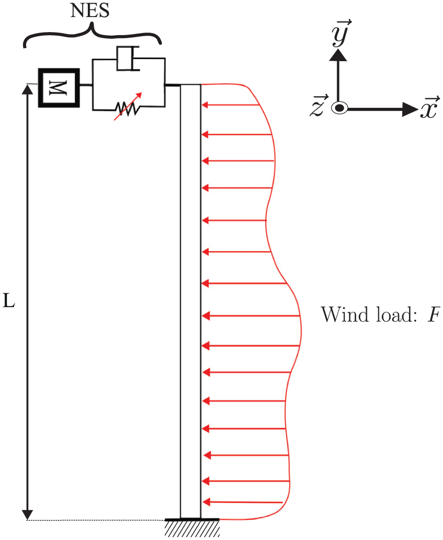
The reference problem: a monopole tower with length L under aerodynamic loading coupled to a nonlinear vibration absorber at y=L.
When dealing with a TMD, the parameters of the absorber are denoted as M tmd , c tmd and k tmd , while for the NES they are denoted as M nes , c nes and k nes , respectively.
Non-dimensionalization of variables and model assumptions
Let us introduce the following dimensionless variables:

By substituting these variables into equation (1) and performing some mathematical manipulations, one obtains the final scaled governing equations for the system as:

We assume that the system’s response is dominated by its k
th
mode, meaning

With:

Vortex-induced vibrations modeling
We consider a monopole with a cylindrical cross-section and length L, subjected to wind flow at a speed U, to which a non-linear absorber is attached, as illustrated in Figure 2. As the wind flows around the structure, vortices can be generated, depending on the velocity of the wind. The relationship between the velocity and the occurrence of vortex shedding can be estimated using the Reynolds number.

A cylindrical monopole tower subjected to cross-flow wind inducing vortex shedding, coupled to a nonlinear vibration absorber for VIVs modeling.
Various approaches have been developed to model VIVs around structures; detailed descriptions are available in the Paidoussis et al. 14 and are summarized in Figure 3.

Different models for VIVs. 14
Type A: Harmonic forced system models, where the force F is independent of the displacement of the body at position y, and therefore it depends only on time, F(t). This is the simplest form of considering the external wind excitation. Type B: Fluidelastic system models, where F depends on the amplitude of the body motion at position y, denoted as

With: ρ
air
the air density, C
D
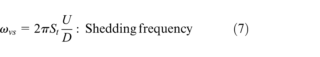
the drag coefficient and D the diameter of the cross section of the monopole. We can see that the vortex shedding frequency depends on the Strouhal number S
t
and f
n
the natural frequency of the structure. When the vortex shedding frequency approaches a natural frequency of the structure, a resonance phenomenon occurs, causing the monopole to vibrate with higher amplitudes. Since the harmonic forcing model does not capture the fluid-structure interaction, we need to calculate the velocity at which the vortex shedding frequency matches one of the natural frequencies of the monopole, thus:

The values in Table 1 correspond to the aerodynamic parameters used. The drag coefficient is based on studies from the Facchinetti et al. 42 and Dai et al., 43 while the Strouhal number is taken as ∼0.21, consistent over a wide Reynolds number range. 44
Parameters for the forcing term amplitude.

The expression of the force in equation (6) can finally be replaced by its dimensionless form

With the amplitude γ defined as follows:
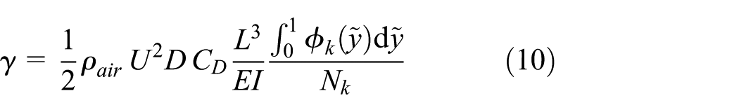
And:

The linear problem
We begin by addressing the linear problem. To this end, we treat the governing equations presented in equation (5). The linear problem is divided into two parts:
The system without the attached absorber.
The system coupled with a linear absorber.
By assuming a solution in the form of a separable function:

The analytical expression for the monopole without the attached absorber can be derived by assuming
Similarly, an analytical approach can be employed to solve the coupled system with a linear absorber. By selecting the

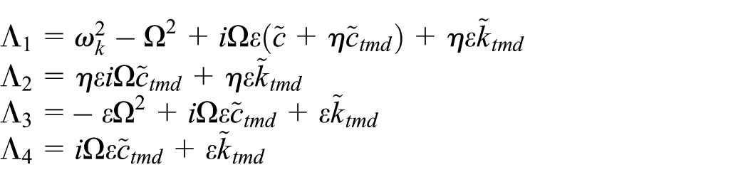
Where:
The nonlinear problem
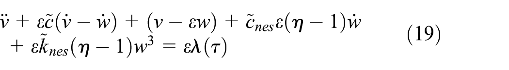
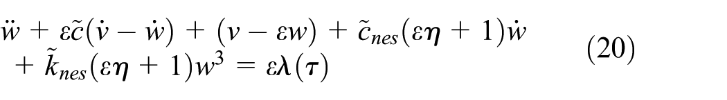
Let us now consider the monopole coupled with a nonlinear absorber, specifically a purely cubic NES. The governing equations are obtained by replacing the linear absorber term in the system of equation (5), namely the function


Before proceeding to solve the problem, we will perform a change of coordinates and express our variables in terms of the center of mass coordinates and relative displacement:


After a few algebraic manipulations, we obtain the expressions for q
n
and
With,
Methodology for treating the nonlinear problem
To treat the nonlinear problem, we will use the Complexification Averaging Method (CX-A). 45 This method combines Manevitch’s complex variables approach with the classical Method of Multiple Scales, allowing us to study the system’s dynamics across different time scales.
We will therefore introduce the complex variables and their conjugate expressions:

After this, we rewrite equations (19) and (20) in terms of complex variables and then apply Galerkin’s method to project the two main equations onto the first harmonic. Using this technique, we express the system dynamics by assuming that the first harmonic represents the predominant excitation 46 :

After applying this technique to the equations and developing the cubic term, we obtain:


We will now use the Method of Multiple-Scales
47
to study the dynamic behavior of the system around the 1:1 resonance on different time scales:
Dynamics of the system on the fast time scale
For the fast time scale, we develop the equations (23) and (24) up to order

The condition for the fixed points of the system is given by:

We note that imposing this condition also enforces the condition:
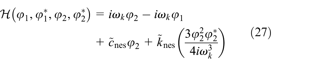
The SIM also provides insight into all possible system responses and is independent of external excitations, as we will demonstrate by solving the equation that imposes the condition for the fixed points:

Substituting this expression back into the SIM equation (27), and after a few mathematical manipulations, we obtain the two expressions:

Noting that:

Noting that the perturbation parameter is very small compared to the main parameter:
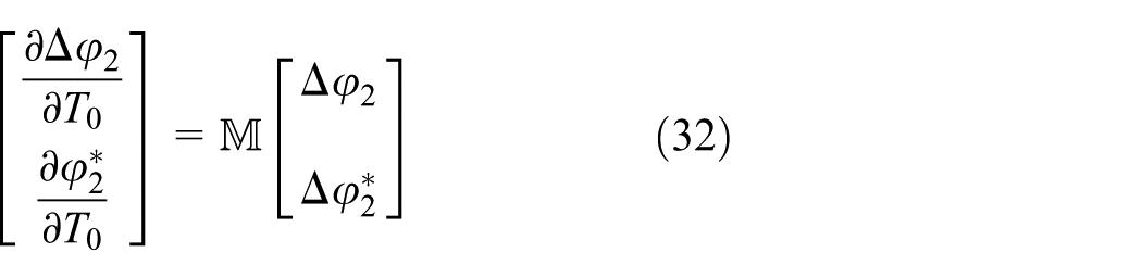
After a few manipulations, and considering the conjugate complex part as well, we will obtain the following system:

This expression can be rearranged and represented in matrix notation:
For the stability of the SIM, we define the condition based on the spectrum of the matrix
The sign of the real part of the eigenvalues of
Dynamics of the system on the slow time scale
We will then analyze the dynamics of the system on a slow time scale by developing our equations up to
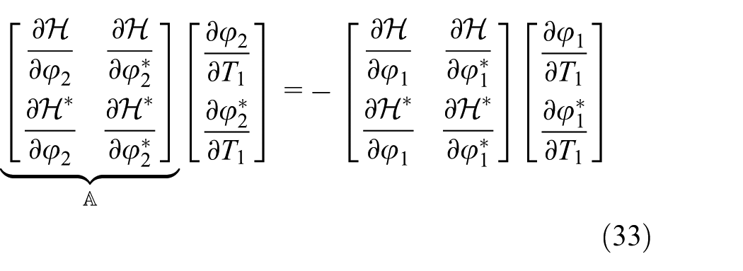
Generally, the equilibrium points of a dynamic system are determined by the condition
The terms of matrix
Singular points:

Equilibrium points

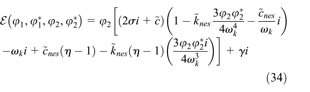
We can begin by determining the singular points by calculating the expression
The critical points are given by the two roots of this equation. To find the equilibrium points, we solve equation (34), by considering the condition

We then determine the coefficients α1, α2, α3, and α4:

By determining the real roots of the polynomial equation (38), we can identify the equilibrium points of the system for N2 and substituting these values into the SIM equation (29) will then allow us to find the equilibrium points for N1. Furthermore, based on the stability analysis conducted earlier, we can distinguish between stable and unstable equilibrium points. It is important to note that σ represents the detuning parameter. Consequently, equilibrium points will be determined over a range of σ values. Specifically, a particular value of σ= 0 corresponds exactly to the
Results
In this section, results obtained from the analytical developments in Section 4 are presented. These results are then compared with those from the numerical integration of the system of equations (19) and (20) for validation purposes.
Analytical results
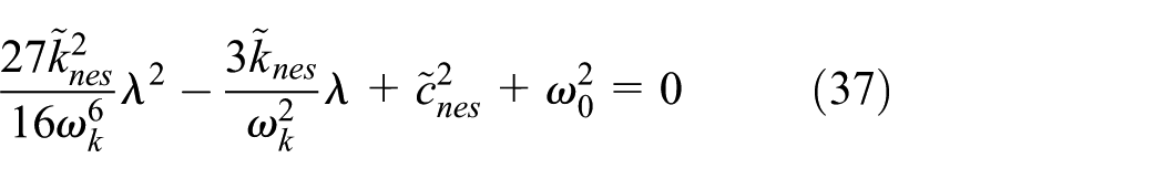
The set of parameters described in Table 2 is selected to show our analytical results. We will first present the results for the SIM, provided by equation (29). In Figure 4, the unstable region is clearly visible and is bounded by the two singular points identified in equation (37).
Parameter values used in the analysis.


Representation of the SIM obtained from equation (29) with defined stable and unstable regions, based on the NES parameters listed in Table 2.
In Figure 5 we show the influence of the damping coefficient ξ
nes
on the SIM behavior. When the value of

SIM for varying values of the damping coefficient ξ nes .
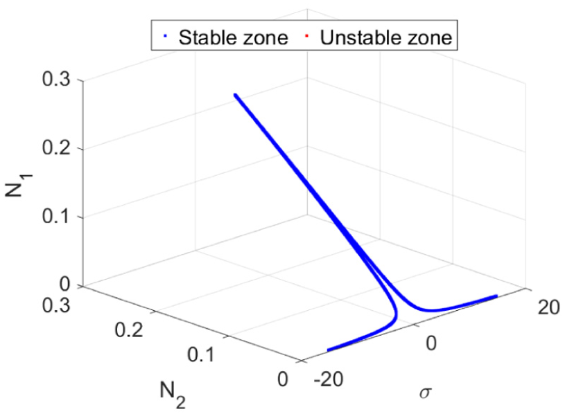
Three-dimensional representation of the equilibrium points of the system (N1, N2, σ) for the forcing amplitudes γ= 0.05.

Three-dimensional representation of the equilibrium points of the system (N1, N2, σ) for the forcing amplitude γ= 1.

Three-dimensional representation of the equilibrium points of the system (N1, N2, σ) for the forcing amplitude γ= 2.
For a given forcing value, detached branches known as isola appear (Figures 9 and 10). The emergence of an isola depends on the amplitude of the external excitation for a given set of system parameters, for example, the rigidity of the nonlinear absorber. 49 Increasing the amplitude of excitation will cause the isola to merge with the main branch of equilibrium points (Figures 11 and 12).

Two-dimensional representation of the equilibrium points of the main system N1 for the forcing term γ= 1.
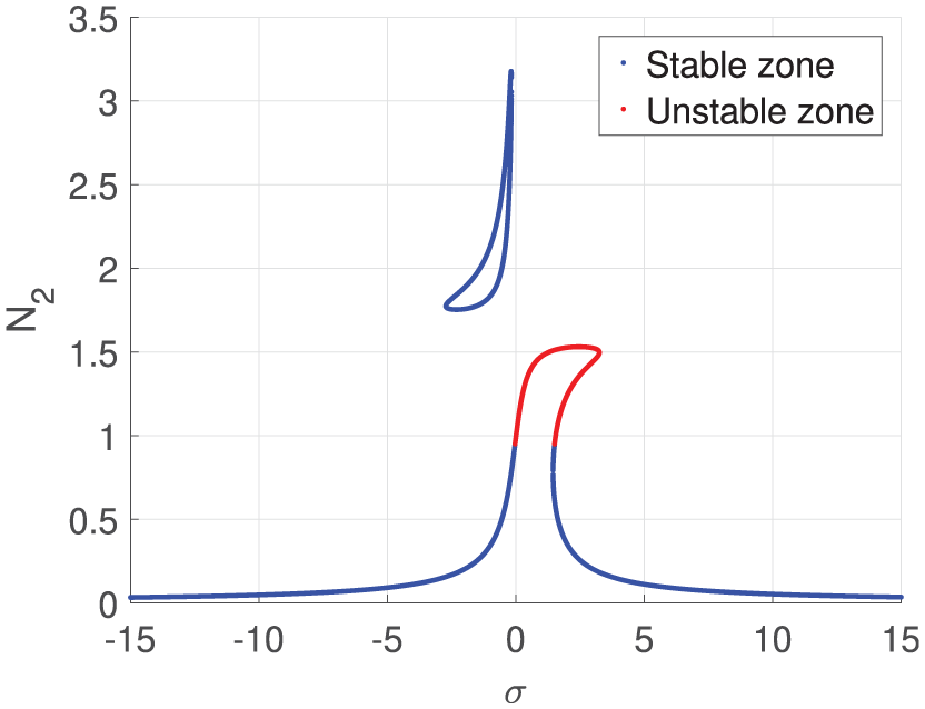
Two-dimensional representation of the equilibrium points of the absorber N2 for the forcing term γ= 1.

Two-dimensional representation of the equilibrium points of the main system N1 for the forcing term γ= 2.

Two-dimensional representation of the equilibrium points of the absorber N2 for the forcing term γ= 2.
Validation of the analytical model
For the validation of the analytical results, the system of equations (19) and (20) is solved using MATLAB’s ODE45 solver. The simulations are performed over the time interval
Initial conditions for each regime.

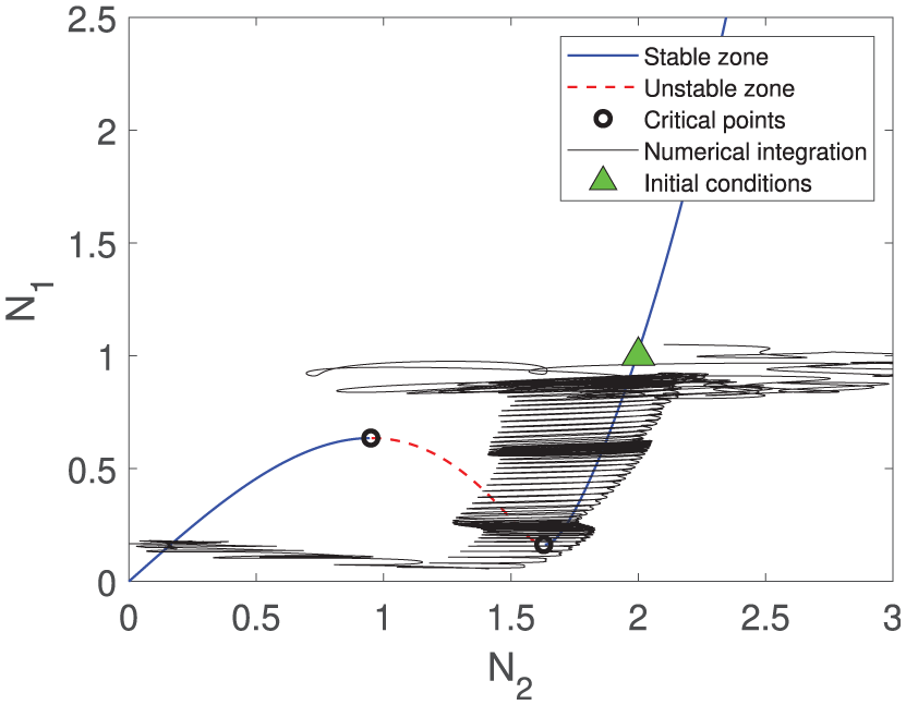
By varying the initial conditions of N1, N2 and the detuning parameter σ, we numerically recover the dynamical regimes predicted by the equilibrium points in Figures 9 and 10, confirming the model’s validity. Starting from the initial conditions
System response validation (periodic regime): SIM evolution for
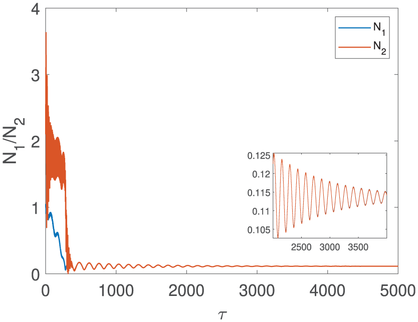
System response validation (periodic regime): final amplitudes N1 and N2 versus scaled time τ.

System response validation (quasi-periodic): SIM evolution for

System response validation (quasi-periodic regime): final amplitudes N1 and N2 versus scaled time τ.
To validate the higher branches, we use initial conditions

System response validation (isola): SIM evolution for

System response validation (isola): final amplitudes N1 and N2 versus scaled time τ.
The Table 4 summarizes the results obtained for each regime. The strong agreement between the analytical predictions and the numerical simulations validates the accuracy of our analytical model. We now proceed to apply this model to a practical case study.
Comparison between Ana. predictions and Num. results.

Ana.: analytical; Num.: numerical.
Application to the case of the Sweetsburg monopole tower
The previously outlined analytical approach is applied to the Sweetsburg monopole telecommunications tower in Quebec, composed of three segments with varying cross-sections. For this study, a simplified model with an equivalent cross-section and moment of inertia is used.51,52 These methods provide a single equivalent inertia that represents the flexural stiffness of the entire non-uniform structure as if it were a uniform beam. The equivalent diameter is calculated as a weighted sum of the section diameters reduced to their lengths, and the equivalent moment of inertia is derived from the lengths and individual moments of inertia of each segment. Applying this method, we obtain the equivalent parameters for the Sweetsburg monopole summarized in Table 5.
Material and geometrical properties of the equivalent model of the Sweetsburg monopole tower.

Where E is the Young’s modulus, L the length, ρ the density, ξ0 the damping coefficient, S the cross-sectional area, and I the second moment of area (moment of inertia) about the flexural axis. For this case study, the analytical model is complemented by a numerical model and a finite element model developed in Code_Aster. 53 The damping coefficient was determined using the critical damping condition:

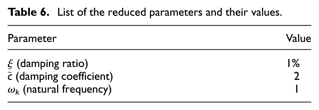
Where, ω k denotes the system’s natural frequency, M the equivalent modal mass, and ξ the damping coefficient of the considered structure. By scaling the parameters from Table 5, we maintain the intrinsic characteristics of the monopole, including Young’s modulus, density, cross-sectional area, and the second moment of area. The reduced parameters are shown in Table 6.
List of the reduced parameters and their values.
We then calculate and plot the natural frequencies of the monopole. These frequencies, obtained using both analytical and finite element approaches, show close agreement, as summarized in Table 7, which serves to validate the models. Furthermore, the first three mode shapes from both methods are visualized in Figure 19, further confirming the consistency between the results.
Comparison of FEM and analytical natural frequencies.


Three first mode shapes obtained from the analytical and FE model: normalized amplitude
The analytical calculations of the modes are presented in Appendix C. After determining the natural frequencies, the associated wind speeds can be computed using equation (8) as derived in Section 2. Using these wind speeds, we subsequently compute the associated wind forces and their scaled values γ, as shown in Table 8.
Wind speeds U, natural frequencies f, equivalent force F x , and scaled value γ for the Sweetsburg monopole.

We will conduct a comparative study on the control of VIVs using both a linear absorber, the TMD, and a nonlinear absorber, the NES. The design of the TMD is based on optimal frequency and damping. For our study, the optimal parameters are determined based on the Den Hartog criterion, 19 which is written as follows:
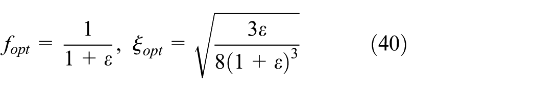
With
Design and optimisation of the NES
We now proceed with the design and optimization of the NES. Theoretically, three key parameters influence the NES design: mass (M
nes
), stiffness (K
nes
), and damping (c
nes
). In our case, the mass ratio between the NES and the modal mass of the monopole is fixed at
The stiffness K nes must be chosen such that the unstable regions in the SIM are activated for a given excitation amplitude and frequency.
The stiffness K nes must be selected to ensure that all points in the SIM (equilibrium points) remain below 70% of the maximum amplitude observed in the system without a coupled absorber.
We will focus here on a wind speed corresponding to the first natural frequency of the monopole, that is,
List of the physical parameters for the NES.

From Figure 20, we observe that with the NES parameters presented in Table 9, the amplitude of the system coupled to the NES remains well below 70% of the maximum amplitude of the system without the NES, when we are at the exact

Amplitude response of the monopole with and without NES at a wind speed of

SIM at a wind speed of

Amplitude response of the monopole with and without NES at a wind speed of

SIM at a wind speed of
Next, we present the time response and the SIM of the coupled system at a wind speed of

Time response of the Sweetsburg monopole under vortex shedding at

SIM of the system for the Sweetsburg monopole under vortex shedding at a wind speed of
Finite element implementation using Code_Aster
The monopole tower is modeled in Code_Aster using 1D beam elements based on the Euler–Bernoulli beam theory, as described in Section 1 and illustrated in Figure 1, with clamped-free boundary conditions allowing only small displacements. The boundary conditions in this study are simplified, as our primary goal is to investigate the control of VIVs using passive absorbers. Ideally, soil–structure interaction or other general elastic interactions should also be considered.54,55 The cubic NES is modeled as a system comprising two linear springs and a central mass, shown in Figure 26. The springs are modeled as discrete elements under the assumption of large displacements. A static analysis with the application of gravitational force was conducted to obtain the force-displacement relationship shown in Figure 27. The properties of the linear springs in Code_Aster were chosen to achieve the desired cubic stiffness. The corresponding parameters used for the NES are the same as those listed in Table 9, while the TMD parameters are presented in Table 10. We used the same mass of
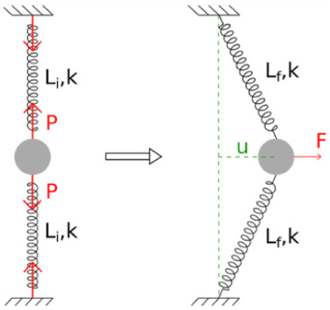
Working principle of the cubic NES. 56
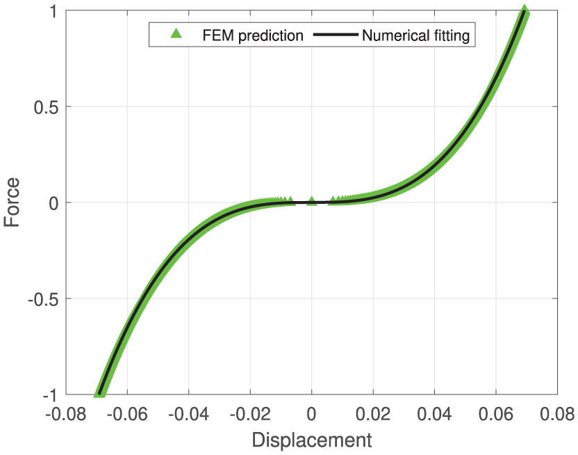
Force-displacement relation for the cubic NES obtained in Code_Aster.
Physical parameters of the TMD used in Code_Aster.

A dynamic nonlinear analysis is performed in Code_Aster using the DYNA_NON_LINE time scheme to simulate the system’s behavior under transient loads for at least 2000 s. We use an adaptive time-stepping method for our simulations. The AUTO method in the DEFI_LIST_INST function enables Code_Aster to automatically adjust the time step size based on a threshold event. The minimum and maximum step times are defined as 10−3 and 10−1 s, respectively, ensuring accuracy and stability. Time integration is carried out using the Newmark method in displacement form, and the solution employs the Newton method with a tangent matrix., applying a convergence criterion based on a maximum number of iterations. Convergence is controlled by a maximum of 500 global iterations (ITER_GLOB_MAXI) and 250 elastic global iterations (ITER_GLOB_ELAS), which are considered appropriate for the model under study.
The evolution of the system’s amplitude as a function of σ is plotted in Figure 28, from which we compare the results from the analytical (continuous line), numerical integration (□), and finite element methods (
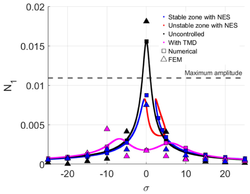
Frequency response of the Sweetsburg monopole at a wind speed of
For the system response with NES, the amplitude considered is that corresponding to the maximum amplitude of the quasi-periodic response. It can be seen from the same figure that, compared to the NES, the TMD is more effective at exact

Effects of changing the excitation frequency of the monopole on the performance of passive absorbers:
Figure 30 shows the time response of the system, illustrating only its steady-state behavior. The maximum amplitude within this range is determined by computing the mean value of the time-response envelope. As can be seen, the system exhibits quasi-periodic behavior, that is, in strong agreement with the predictions of the numerical model. Furthermore, pronounced attenuation of the response amplitude is evident when the system is coupled with the NES.

Time response of the Sweetsburg monopole under vortex shedding at
Conclusion
The paper investigates the control of vortex-induced vibrations on monopole telecommunication towers using nonlinear passive absorbers. Following the development of the system’s mathematical model and its analytical formulation, a case study has been conducted on the Sweetsburg monopole tower. A comparison has also been made between the performances of the nonlinear energy sink and the tuned mass damper in controlling vortex-induced vibrations. The analytical approach enables us to determine the nonlinear dynamical characteristics of the monopole coupled to the nonlinear energy sink at different timescales, such as the slow invariant manifold, the equilibrium points, and singular points, forming the basis for designing an effective nonlinear energy sink. Numerical methods have validated the analytical results and established a benchmark for comparison. Finite element analysis further confirmed the consistency of both approaches. The results highlight the potential of nonlinear energy sinks as an effective solution for controlling vortex-induced vibrations over a wide range of frequencies; however, their performance depends strongly on the activation of a threshold covering unstable zones and bifurcations. Therefore, the appropriate selection of the absorber stiffness during the design process is crucial for overcoming this issue.
Footnotes
Appendices
Acknowledgements
The authors would like to thank the Auvergne Rhône Alpes region for partially funding this work. They also acknowledge the contributions of Dany Toulouse and Samuel Jubinville-Baron from YRH for the discussions on the subject of telecommunication tower vibration control and for facilitating access to the documents regarding the Sweetsburg tower.
Handling Editor: Sharmili Pandian
Funding
The authors received no financial support for the research, authorship, and/or publication of this article.
Declaration of conflicting interests
The authors declared no potential conflicts of interest with respect to the research, authorship, and/or publication of this article.