Sage Journals: Discover world-class research

Abstract

To study the vortex-induced vibration behaviors of tube arrays with large pitch-to-diameter ratio values, an experiment has been conducted by testing the responses of an elastically mounted tube in a fixed normal triangular tube array with five rows and a pitch-to-diameter ratio value of 2.5 in a water tunnel subjected to cross-flow. The amplitude curves, power spectral density, and response frequencies were obtained in both in-line and transverse directions through the experiment. The results show that the responses obtained from the in-line direction are quite different from those obtained from the transverse direction. In the in-line vibration, there were two excitation regions, yet in the transverse vibration, there was only one excitation region. Moreover, in the in-line vibration, two obvious prominent peaks can be observed in the power spectral density of the vibration signal. The second prominent peak is a subharmonic peak. The frequency corresponding to the subharmonic peak was nearly twice as high as that corresponding to the first peak. However, in the transverse vibration, only a single broad peak existed in the power spectral density of the vibration signal. The hysteresis and the “lock-in” phenomena appeared in both the in-line and transverse vibrations. The results of study are beneficial for designing and operating devices mounted with large pitch-to-diameter ratio tube arrays, and for further research on the vortex-induced vibration of tube arrays.

Keywords

Vortex-induced vibration vortex shedding tube array in-line vibration transverse vibration

Introduction

Vortex-induced vibration plays an important role in the field of fluid–structure interactions. The case of the vortex-induced vibration of tube arrays is one of the most basic and remarkable cases in the general subject of fluid–structure interactions. It is of theoretical and practical value to analyze the tube arrays vibration in many fields of engineering, such as in the designs for heat exchangers, cooling systems for nuclear power plants, offshore structures, buildings, chimneys, power lines, struts, grids, screens, and cables, in both air and water flow.^1–7

Vortex-induced vibration is caused by the vortexes shedding behind the tube and takes place when the vortex shedding frequency is close to the natural frequency of the tube. Among the whole tube-like structures, vortex-induced vibration could be prominent in the cases of a single tube and tube arrays with large pitch-to-diameter ratio (P/D) values. In the case of tube arrays with small P/D values, the instability behaviors are often caused by fluid-elastic instability and the vortex formation is impeded by neighboring tubes.^8–10

In previous decades, many scholars have devoted themselves to discovering the essence of vortex-induced vibration though a single cylinder. Couder and Basdevant¹¹ carried out an experimental and numerical study of vortex couples in two-dimensional flows. Williamson¹² tested oblique and parallel modes of vortex shedding in the wake of a circular cylinder at low Reynolds numbers. Blackburn and Henderson¹³ simulated the lock-in behavior in vortex-induced vibration, while Khalak and Williamson¹⁴ investigated the dynamics and fluid forcing on an elastically mounted rigid cylinder. In recent years, Lam and Dai¹⁵ studied the formation of vortex street and vortex pair from a circular cylinder oscillating in water. Govardhan and Williamson¹⁶ defined the “modified Griffin plot” in vortex-induced vibration. Vandiver et al.¹⁷ investigated traveling waves on a long flexible cylinder excited by vortex shedding, while Tang et al.¹⁸ simulated vortex-induced vibration with three-step finite element method and arbitrary Lagrangian–Eulerian formulation. Gallardo et al.¹⁹ simulated turbulent wake behind a curved circular cylinder.

The study of vortex-induced vibration on tube arrays is also very important in theory and industrial applications where operational costs need to be reduced. However, vortex-induced vibration on tube arrays is more complex than that in the case of a single tube, resulting from the fact that the vibrating tube can be influenced by the wake of the tubes in the upstream. Many scholars have paid attention to the case of tubes in tandem arrangements^20,21 which can be used for simplifying the problem. Bokaian and Geoola,²² Brika and Laneville,²³ Hover and Triantafyllou,²⁴ and Assi et al.^25,26 studied the vibration response of a downstream tube excited by the wake of a fixed upstream tube. Huang and Herfjord²⁷ investigated the forces and motion responses of two elastically mounted tubes which were arranged in tandem. Oviedo-Tolentino et al.²⁸ tested the vortex-induced vibrations of a collinear array of 10 identical flexible cylinders. Zhao²⁹ simulated flow-induced vibration of two rigidly coupled circular tubes in tandem and side-by-side arrangements. However, neither the case of a single tube nor that of two tubes arranged in tandem can accurately represent the vortex-induced vibration in a real tube bundle, because differences in tube array patterns, array pitch-to-diameter ratios P/D, the orientation of the tubes relative to the oncoming flow, the Reynolds number, and so on can influence the vibration response of tube arrays excited by vortex shedding. Experimenting in a real tube array, not a single tube or two tubes arranged in tandem for studying the vortex-induced vibration in tube arrays is, therefore, important. Fitz-Hugh³⁰ measured Strouhal numbers of a series of fixed tube arrays with different P/D values and in different patterns. Paidoussis³¹ cited various industrial problems resulting from vortex-induced vibration in heat exchangers and nuclear reactors. Ziada and Oengören³² investigated the vorticity shedding and acoustic resonance mechanisms in parallel triangle tube arrays with a series of pitch ratios, which were mounted rigidly, and showed the flow patterns by the fluid visualization technology. Although some results could be received among these studies, the specific research about the vortex-induced vibration of tube arrays with large P/D values is still lacking.

With this background, an experiment has been completed by testing the responses of a normal triangular tube array with a P/D value of 2.5 in a water tunnel under both increasing and decreasing cross-flow velocities. Responses in both the in-line and transverse directions were obtained. The experimental data were analyzed in terms of various aspects, such as time–histories’ displacement analysis, spectrum analysis, and response frequency analysis. Through these analyses, the amplitudes, power spectral density functions, response frequencies, and so on were obtained. Our findings can enrich the database about the vortex-induced vibration and offer some valuable guidance for the operation and design of devices with large P/D tube arrays, such as offshore platforms and pile foundations for wharf among offshore structures. Moreover, the study will be beneficial for further research about the vortex-induced vibration of tube arrays.

Experiment details

Experimental apparatus and instrumentation

Figure 1 shows a schematic of the experimental loop used in this work, which is widely applied in the field of the cross-flow vibration research of tube arrays.^9,33–37 In this study, water was pumped through a tank, electromagnetic flowmeter, and two valves, and then flowed past steady flow plates for stabilizing the incoming flow before entering the test section.

Figure 1.

A schematic diagram of the experimental loop.

The test section, which was made of stainless steel, had internal dimensions of 0.14 m × 0.14 m and a length of 2.602 m and contained a tube array shown in Figure 2. The center of the tube array was at 1.455 m downstream of the top of the steady flow plates. The tube array, which consisted of an array of aluminum tubes with an outer diameter of 0.012 m, an inner diameter of 0.010 m, and a length of 0.130 m, had a normal triangular arrangement. Gelbe et al.¹⁰ pointed out that undisturbed Karman vortex streets can only develop when large pitch-to-diameter ratios (P/D) are involved, and vortex formation is impeded by neighboring tubes with small P/D, that is, 1.1 < P/D < 2.0. According to their view, the effect of neighboring tubes on vortex formation can become increasingly weaker as the P/D value increases. As a result, the vortex-induced vibration behaviors of tube arrays with too large P/D can be quite similar to those observed for an isolated tube.

Figure 2.

Schematic of the test section of the experimental apparatus.

In order to avoid the cases above, a series of experiments about 2.3 ≤ P/D ≤ 2.9 were completed. The regularities of the results corresponding to these P/D values are similar. For the limitation of the thesis, in this article, we only chose the experimental results corresponding to a P/D value of 2.5, which can best fit the vortex-induced vibration behaviors of tube arrays. The vortex-induced vibration behaviors shown in section “Results and discussions” were not similar to those observed in an isolated tube. There were five rows, with alternately four or five tubes per row. Similar to Khalifa et al.³⁸ and Mahon and Meskell,³⁹ the monitored tube was mounted in the center of the tube array elastically, while others were fixed at the channel walls of the test section with bolts at two ends to create rigid tubes.

As shown in Figure 3, the monitored tube was mounted elastically and was equipped with two stainless steel piano lines, two screw tubes, two screw nuts, two springs, and two pins. One endpoint of every stainless steel piano line was fixed to the monitored tube, and the other endpoint was fixed to a pin. In order to adjust the natural frequency of the vibration system, screw nuts were used to adjust the springs. The displacement mechanism of the monitored tube was derived from Joo and Dhir,⁴⁰ Mitra,⁸ Cagney and Balabani,⁴¹ and so on. The measured tube was free to move simultaneously in both the transverse and in-line directions. Prior to the water tunnel tests, the frequency and damping of the monitored tube were measured using the logarithmic decrement technique. The data are summarized in Table 1. The mass ratio m^* shown in Table 1 is calculated using the equation below

m^{*} = \frac{M}{\frac{π}{4} ρ D^{2} L}

(1)

Figure 3.

Half side view of the installation schematic diagram of the monitored tube.

Table 1.

Monitored tube data without flow.

Name	Data
Natural frequency in water in the in-line direction, f_{n_x}	11.332 Hz
Natural frequency in water in the transverse direction, f_{n_y}	11.332 Hz
Damping ratio in water in the in-line direction, ξ_x	5.10%
Damping ratio in water in the transverse direction, ξ_y	5.13%
Structural mass (including acceleration transducers inside), M	0.0220 kg
Mass ratio m*	1.5
Mass damping in still water in the in-line direction	0.0765
Mass damping in still water in the transverse direction	0.0770

The mass damping values shown in Table 1 can be calculated by the equation below

\frac{m (2 π ζ)}{ρ D^{2}} = \frac{π}{4} m^{*} \times 2 π ζ = \frac{π^{2} m^{*} ζ}{2}

(2)

m = \frac{M}{L}

(3)

where M is the mass of the monitored tube (including acceleration transducers inside), ρ is the density of the fluid, D is the outer diameter of the monitored tube, L is the length of the tube, m is the mass of the monitored tube in unit length, and ζ is the damping ratio of the monitored tube in still water in the in-line or transverse direction.

Acceleration transducers with sensitivity of 1.71 pC/g and frequency response of 1 Hz–20 kHz were chosen to obtain the displacement signals directly and simultaneously.^9,42–44 The output signal was calibrated to have a linear relationship to the input signal. Two acceleration transducers installed inside the monitored tube at mid-span were treated as part of the monitored tube during the experiment. Their orientations were adjusted such that they were sensitive to tube vibrations only in the in-line (X) and transverse (Y) directions, respectively. The process of collection and analysis of signals is shown in Figure 4. The output signals of the two acceleration transducers were collected using a dynamic signal collector with a 24-bit analog-to-digital converter. The dynamic signal collector could transform the output signals to voltage signals at first, and then it could integrate the voltage signal twice to provide a displacement signal. All signals were high-pass filtered in post-processing at 1.2 Hz to prevent “blow-up” that commonly occurs due to low-frequency noise when converting acceleration to displacement. The cut-off frequency of 1.2 Hz is significantly lower than the response frequencies obtained from the whole experiment. At each given flow velocity, the in-line and transverse displacement signals were digitized simultaneously at a sampling frequency of 200 Hz, and the frequency spectra and response amplitudes recorded were the result of 64 sample averages which proved to be sufficient in achieving a steady state for each flow velocity. Meanwhile, during the experiments, the anti-aliasing filter was in the state of turning on all the time. All data were transmitted to a personal computer for data storage and further processing. The software MATLAB was used in analyses of the data.

Figure 4.

Collection and analysis of the digital signal process.

Before experiments, the output signals of the whole data acquisition system were calibrated just as Lin and Yu⁹ have done. The monitored tube with two acceleration transducers inside was given a circular motion. The typical time–history curves and calibration curves of the two acceleration transducers are shown in Figures 5 and 6, respectively. The amplitudes of the sinusoidal output signals for the in-line and transverse directions were recorded and then plotted against the standard vibration amplitude which was the radius of the circular motion. The calibration curves can be determined as

A = 1.000 B + 0.0536

(4)

in the in-line direction, and

A = 1.000 B + 0.0738

(5)

in the transverse direction where A represents the standard vibration amplitude, and B represents the measured vibration amplitude obtained by the whole data acquisition system. As shown in Figure 6, the measured amplitude signals were all linear to the standard amplitude signals, so the measured amplitudes can represent the vibration amplitudes linearly in the whole experiment.

Figure 5.

Typical time–history curves at the time for calibration of two acceleration transducers: (a) in-line direction and (b) transverse direction.

Figure 6.

Fitted curves for calibration of two acceleration transducers: (a) in-line direction and (b) transverse direction.

Experimental procedure

The freestream velocity in front of the tube array in the test section is calculated using the equation

U_{\infty} = \frac{V}{3600 ab}

(6)

where U_∞ is the freestream velocity in front of the tube array in the test section (m/s), V is the flow rate (m³/h), a is the length of the cross section of the test section (equal to 0.14 m), and b is the width of the cross section of the test section (equal to 0.14 m).

According to equation (6), the centrifugal pump is able to deliver up to 65 m³/h, which makes the maximum averaged water freestream velocity in front of the tube array in test section reach 0.921 m/s by the internal dimensions of the test section. The corresponding maximum Reynolds number Re is 1.098 × 10⁴, based on the freestream velocity and the outer diameter of the experimental tubes. The flow rate first increased from 0 to the maximum with an approximate step size of 1.5 m³/h which is equivalent to 0.0213 m/s in the test section, and then decreased to 0 in the same way. During the whole experiment, the freestream velocity U_∞ first increased from 0 to 0.921 m/s with an approximate step size of 0.0213 m/s, and then decreased to 0 in the same way. Meanwhile, the Reynolds number Re first increased from 0 to 1.098 × 10⁴ with an approximate step size of 0.2539 × 10³, and then decreased to 0 in the same way. After reaching a steady state for each flow rate, the measurement was initiated.

Results and discussions

Response amplitude

Figure 7 shows the response amplitudes of the monitored tube in the two-dimensional plane when flow velocity increased and decreased comprehensively. The response curves of the in-line oscillation are compared with those of the transverse oscillation, and the root mean square (RMS) tube amplitude (expressed as a percentage of the tube diameter) is plotted against the reduced pitch flow velocity U^*, which is calculated through the equations below

U_{P} = \frac{P}{P - D} U_{\infty}

(7)

U^{*} = \frac{U_{P}}{f_{n} D}

(8)

where U_∞ is the freestream velocity in front of the tube array, P is the pitch of the tube array, D is the outer diameter of the tube, U_p is the pitch flow velocity, and f_n is the natural frequency of the tube in water in the in-line or the transverse direction. During the experiments, the Reynolds number Re is simply proportional to reduced pitch flow velocity U^*.

Figure 7.

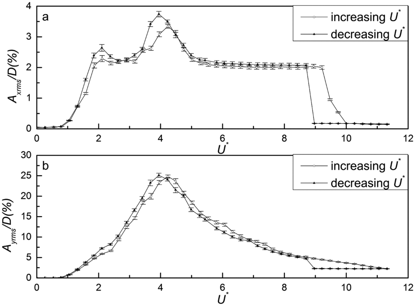
The dimensionless response amplitude of the monitored tube in the two-dimensional plane versus reduced pitch flow velocity U^* with error bar: (a) in-line direction and (b) transverse direction.

Figure 7(a) shows that there are two humps in the cases of both increasing flow velocity and decreasing flow velocity, respectively, similar to the experimental results obtained by King et al.⁴⁵ and Okajima et al.⁴⁶ This indicates that there are two excitation regions in the cases of both increasing and decreasing flow velocities, respectively. Especially, the excitation regions corresponding to the case of decreasing flow velocity are more evident than the excitation regions corresponding to the case of increasing flow velocity. This indicates that when the instability behavior has occurred, decreasing the flow velocity may cause the devices with tube arrays to vibrate more intensely.

However, in Figure 7(b), only a single hump is observed in the cases of both the increasing flow velocity and the decreasing flow velocity, indicating that only a single excitation region exists in the cases of both increasing and decreasing flow velocities. No matter in the in-line direction or in the transverse direction, the response amplitude curves reach the maximum at same U^*, which are U^* = 4.238 in the case of increasing flow velocity, and U^* = 3.946 in the case of decreasing flow velocity. When U^* < 4.238 in the case of increasing flow velocity, the response amplitude obtained from transverse vibration increases evenly without a saltation as the flow velocity increases. In the same way, when U^* < 3.946 in the case of decreasing flow velocity, the response amplitude obtained from transverse vibration also decreases evenly without a saltation as the flow velocity decreases. In the case of increasing U^*, once the in-line and transverse response amplitudes reach the maximum values, they will decrease as the flow velocity increases. These characteristics all do not fit the common characteristics of fluid-elastic instability.

Any increase or decrease within the response curves may be a sign of transition in the response. More explanations about the differences between the amplitude responses obtained from the in-line and transverse vibrations are discussed in section “Power spectral density functions of the monitored tube vibration” through power spectral density functions.

Hysteresis phenomenon

As can be clearly seen in Figure 7(a) and (b), the response amplitude curves for velocity increase and decrease are different. Additionally, when the flow velocity decreases, a hysteresis phenomenon appears in both the in-line and transverse vibrations.

As shown in Figure 7(a), the onset of the second excitation region corresponding to the case of decreasing flow velocity shifts to the lower water velocity range. In Figure 7(b), an evident saltation is found from U^* = 8.971 to U^* = 8.701. Furthermore, whether the direction is in-line or transverse, the U^* value corresponding to the maximum response amplitude values in the case of decreasing flow velocity is less than that in the case of increasing flow velocity. In the U^* ranges, which are lower than the U^* values corresponding to the maximum response amplitude values, the response amplitude curves corresponding to the case of decreasing flow velocity are above those corresponding to the case of increasing flow velocity in the in-line and transverse directions. As a result, a significant hysteresis phenomenon appeared in both in-line and transverse vibrations.

Power spectral density functions of the monitored tube vibration

In-line direction

In order to gain more insights into the vibration characteristics, we calculated a power spectral density function of the vibration signals.

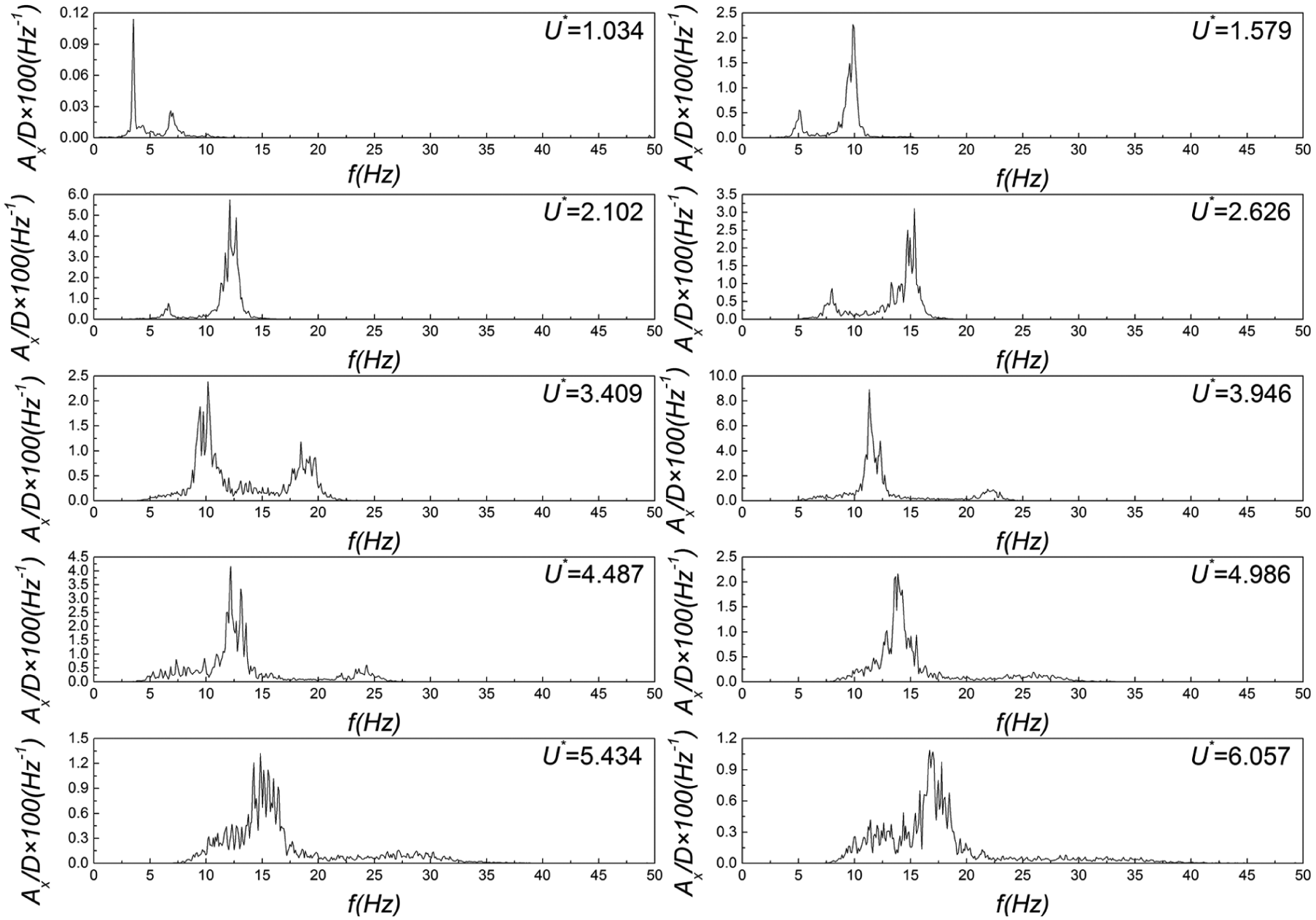
Figure 8 shows the obtained power spectral density functions of the tube vibrations in the in-line direction with increasing flow velocity. Figure 9 shows the obtained power spectral density functions of the tube vibrations in the in-line direction with decreasing flow velocity. Whether the flow velocity is increasing or decreasing, two prominent peaks can be observed when the U^* values are <5 in general. According to Franzini et al.,⁴⁷ the second prominent peak in each power spectral density function is a subharmonic peak. Furthermore, the frequency corresponding to the subharmonic peak is nearly twice as high as that corresponding to the first prominent peak at each U^*. The typical power spectral density function with two prominent peaks is shown in Figure 10.

Figure 8.

Power spectral density of tube in-line vibration amplitude in the case of increasing flow velocity.

Figure 9.

Power spectral density of tube in-line vibration amplitude in the case of decreasing flow velocity.

Figure 10.

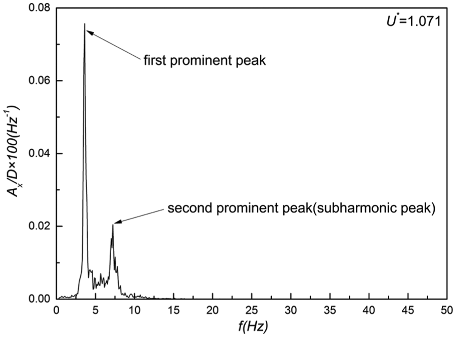
Typical power spectral density: U^* = 1.071 in the case of increasing flow velocity.

With the increasing flow velocity, the two prominent peaks move to higher frequency. In the process of moving, the subharmonic peak first approaches the natural frequency of the monitored tube at U^* = 1.582. As a result, its signal strength increases rapidly and reaches a maximum value at U^* = 2.111. This process corresponds to the first excitation region in the case of increasing flow velocity in Figure 7(a). After this point, as the flow velocity increases continuously, the subharmonic peak moves farther from the natural frequency, so that its signal strength begins to decrease. With the continuous increase in flow velocity, the first prominent peak begins to approach the natural frequency of the monitored tube at U^* = 2.905; similarly, the signal strength of the first prominent peak increases rapidly, and then reaches a maximum value at U^* = 4.238. This process corresponds to the second excitation region in the case of increasing flow velocity in Figure 7(a).

At the time of decreasing flow velocity, the first prominent peak first approaches the natural frequency of the monitored tube, resulting in signal of the first prominent peak becoming stronger and stronger to reach a maximum at U^* = 3.946. Afterward, as the flow velocity decreases continuously, the first prominent peak moves farther from the natural frequency of the monitored tube, so that its signal strength begins to decrease. This process corresponds to the second excitation region in the case of decreasing flow velocity in Figure 7(a). Afterward, the subharmonic peak starts to approach the natural frequency of the monitored tube with the signal becoming increasingly stronger. With the continuous decrease in the flow velocity, the strength of the subharmonic peak begins to decrease after its maximum at U^* = 2.102. This process corresponds to the first excitation region in the case of decreasing flow velocity in Figure 7(a).

According to the discussion above, the two excitation regions in Figure 7(a) are caused by the two prominent peaks in the power spectral density function of tube in-line vibration.

Transverse direction

As shown in Figures 11 and 12, the power spectral density functions of the tube vibrations in the transverse direction are quite different from those in the in-line direction. Unlike Figures 8 and 9, at each U^*, there is nearly only one dominant single broad peak. There are no two prominent peaks, among which the frequency corresponding to the second peak is nearly twice as high as the frequency corresponding to the first peak. This may be the reason why there is only one excitation in the transverse vibration in Figure 7(b). With the increasing flow velocity, the dominant peak moves to higher frequency. At first, the strength of the signal becomes increasingly stronger, eventually reaching a maximum at U^* = 4.238. Afterward, the signal begins to decrease. When the flow velocity is decreasing, the dominant peak moves to the lower frequency. Similar to the case of increasing flow velocity, the strength of the signal becomes increasingly stronger and reaches a maximum at U^* = 3.946, before decreasing gradually.

Figure 11.

Power spectral density of tube transverse vibration amplitude in the case of increasing flow velocity.

Figure 12.

Power spectral density of tube transverse vibration amplitude in the case of decreasing flow velocity.

According to the power spectral density functions obtained from the in-line and transverse vibrations, the differences between the amplitude responses from the two directions are caused by the differences between the frequency variations in the signals, which are obtained from the two directions.

Response frequency

In-line direction

As shown in Figures 8 and 9, there are two prominent peaks in power spectral density function obtained from the in-line vibration at each U^* which is lower than 5 in general; thus, we have plotted the response frequencies corresponding to the two prominent peaks at each U^* in Figures 13 and 14 separately.

Figure 13.

Response frequencies corresponding to the first prominent peaks of the power spectral density functions obtained from the in-line vibrations versus U^*: (a) increasing U^* and (b) decreasing U^*.

Figure 14.

Response frequencies corresponding to the subharmonic peaks of the power spectral density functions obtained from the in-line vibrations versus U^*: (a) increasing U^* and (b) decreasing U^*.

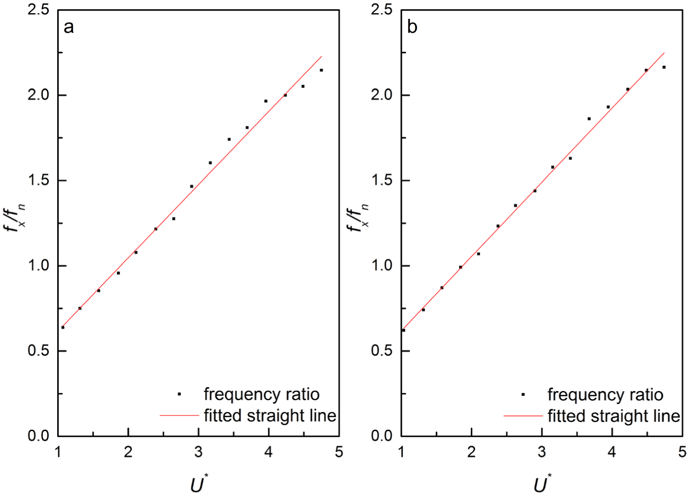
Figure 13 shows the response frequencies corresponding to the first prominent peaks obtained from the in-line vibrations versus U^*. As can be seen in the figure, the response frequency increases with the U^* nearly linearly in the cases of both increasing and decreasing U^*. When 3.959 ≤ U^* ≤ 4.488 in the case of increasing U^* and 3.673 ≤ U^* ≤ 4.225 in the case of decreasing U^*, the frequency ratio values stay at nearly 1, indicating that the tube oscillation frequency is equal to the natural frequency, and that the “lock-in” phenomenon occurs. Two slope values have been obtained by applying linear relationship to fit the data that are out of the ranges of lock-in to be two straight lines. These values, 0.2497 and 0.2480, correspond to the cases of increasing U^* and decreasing U^*, respectively. In the same way, the R² values are 0.9978 and 0.9979, respectively

S_{t} = \frac{fD}{U_{P}}

(9)

U^{*} = \frac{U_{P}}{f_{n} D} \times \frac{f_{n}}{f_{x}} \times \frac{f_{x}}{f_{n}} = \frac{U_{P}}{f_{x} D} \times \frac{f_{x}}{f_{n}}

(10)

\frac{f_{x} D}{U_{P}} = \frac{f_{x} / f_{n}}{U^{*}}

(11)

According to equations (9)–(11) above, the slope of the fitted straight line can represent an actual Strouhal number. The Strouhal number corresponding to an isolated tube under the Reynolds number in this experiment is estimated to be 0.18 according to the figure drawn by Lienhard.⁴⁸ Additionally, the Strouhal number corresponding to the tube array in this experiment is estimated to be 0.25 according to the figure drawn by Fitz-Hugh.³⁰ The slope values cannot fit the theoretical value of an isolated tube under the Reynolds number in this experiment. In comparison, the slope values can fit the theoretical value of the tube array in this experiment very well, indicating that the vibration of the monitored tube was caused by vortex shedding in the tube array.

By applying the theoretical Strouhal number and the Strouhal number equation, at the point U^* = 3.959 which is the occurrence of lock-in in the case of increasing flow velocity, the calculated vortex shedding frequency is 11.214 Hz; such a value can well fit the frequency corresponding to the first prominent peak in the power spectral density function of the in-line vibration 11.231 Hz very well. At the point U^* = 4.225, which is the occurrence of lock-in in the case of decreasing flow velocity, the calculated vortex shedding frequency is 11.967 Hz; such a value can well fit the frequency corresponding to the first prominent peak in the power spectral density function of the in-line vibration 11.426 Hz very well. All these results above conform to the characteristics of vortex shedding in the tube array.

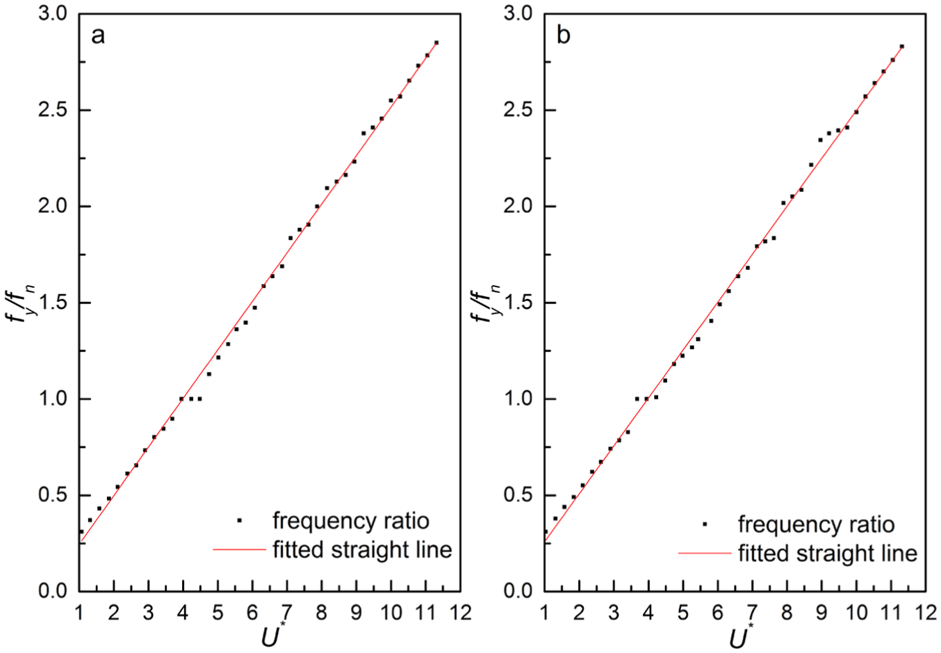
Figure 14 shows the response frequencies corresponding to the subharmonic peaks obtained from the in-line vibrations versus U^*. Considered that the subharmonic peak is not obvious in the U^* range, which is higher than 5, so the maximum U^* value in Figure 14 is set to be 5. Similar to Figure 13, the response frequencies also keep a linear relationship with the U^* values. Two straight lines are fitted, resulting in two slope values, 0.4296 and 0.4358, which correspond to the cases of increasing U^* and decreasing U^*, respectively. Their R² values are 0.9906 and 0.9947, respectively.

Transverse direction

The dominant response frequencies obtained from transverse vibrations versus U^* are shown in Figure 15. These frequencies are extremely similar to the data shown in Figure 13. Regardless of whether U^* increases or decreases, the response frequencies keep a linear relationship with U^* values as a whole. Two slope values, 0.2522 and 0.2489, are calculated from the two fitted straight lines corresponding to the case of increasing U^* and the case of decreasing U^* in Figure 15, respectively. Their R² values are 0.9983 and 0.9978, respectively. The two slope values remain consistent with the theoretical Strouhal number 0.25 for the tube array used in this experiment very well. Furthermore, the lock-in phenomenon also occurred in the transverse vibration. Just like in Figure 13, when 3.959 ≤ U^* ≤ 4.488 in the case of increasing U^* and 3.673 ≤ U^* ≤ 4.225 in the case of decreasing U^*, the frequency ratio values stay at nearly 1. As discussed in section “In-line direction,” by applying the theoretical Strouhal number and the Strouhal number equation, at the point U^* = 3.959, which is the occurrence of lock-in in the case of increasing flow velocity, the calculated vortex shedding frequency is 11.214 Hz. This value can well fit the dominant transverse frequency 11.328 Hz. At the point U^* = 4.225, which is the occurrence of lock-in in the case of decreasing flow velocity, the calculated vortex shedding frequency is 11.967 Hz. This value can well fit the dominant transverse frequency 11.426 Hz. All these results above also conform to the characteristics of vortex shedding in the tube array. Meanwhile, the response amplitude characteristics shown in Figure 7 do not fit the common characteristics of fluid-elastic instability. Synthesizing the results above, fluid-elastic instability did not occur in this experiment.

Figure 15.

Dominant response frequencies obtained from the power spectral density functions of transverse vibrations versus U^*: (a) increasing U^* and (b) decreasing U^*.

As shown in Figure 7, the flow velocity ranges corresponding to the significant large response amplitude of the monitored tube contain the flow velocity ranges which are out of the ranges corresponding to lock-in. It should be caused by the low mass ratio of the monitored tube.

The mass ratio of the monitored tube was 1.5, which was very small. Therefore, the inertia effect of the monitored tube chosen in this experiment was weaker than the tubes with large mass ratios, and the vibration statement of the monitored tube was easier to be influenced by the flow velocity than the tubes with large mass ratios. During our experiment, with the increase in the flow velocity, the frequency of vortex shedding increased following the Strouhal line. Due to the small mass ratio of the monitored tube, the vibration statement of the monitored tube was easy to be influenced by the flow. The monitored tube was excited by the shedding vortexes. As the flow velocity increased, when the frequency of the vortex shedding is approaching the natural frequency of the monitored tube, the response amplitude of the monitored tube continuously grew larger. After the vortex shedding frequency reached the natural frequency of the monitored tube, the vibrating frequency of the monitored tube only stayed for a narrow range of flow velocity and then increased sequentially and obviously as the flow velocity increased, resulted from the small mass ratio of the monitored tube. As the flow velocity increased continuously, the vortex shedding frequency exceeded the natural frequency of the monitored tube and the response amplitude of the monitored tube began to decrease slowly. The case of decreasing flow velocity is similar to the case of increasing flow velocity. Synthesizing the results above, as a result of the low mass ratio of the monitored tube, the flow velocity ranges corresponding to the case of lock-in are narrow and the flow velocity ranges corresponding to the significant large response amplitude of the monitored tube contain the flow velocity ranges which are out of the ranges corresponding to lock-in in our experiments.

Trajectories of the monitored tube

The vibration behavior of the monitored tube can be further understood by examining its trajectories in the fluid flow. Figure 16 shows the trajectories of the monitored tube in the case of increasing U^*, while Figure 17 shows the trajectories of the monitored tube in the case of decreasing U^*.

Figure 16.

Trajectories of the monitored tube in the case of increasing U^*.

Figure 17.

Trajectories of the monitored tube in the case of decreasing U^*.

The variation in the trajectories of the monitored tube can well reflect the variations in the response amplitudes and the dominant vibration frequencies (i.e. the frequency with the maximum amplitude in a power spectral density function obtained from in-line or transverse vibration) of the monitored tube in the in-line and transverse directions. As shown in Figure 16, with the increase in the flow velocity, the trajectories of the monitored tube are initially like a figure of “8” clearly, indicating that the dominant frequencies in the in-line vibrations are the subharmonic frequencies that are twice as high as the dominant frequencies in the transverse vibrations; furthermore, the signal strength of the subharmonic peaks is much stronger than that of the first prominent peaks in the power spectrum density functions of the in-line vibrations. However, this phenomenon does not last all the time. As the flow velocity increases further, the shape of the trajectories of the monitored tube is shifting from an 8 to an approximate ellipse, indicating that the relative signal strength of the first prominent peaks vis-a-vis the signal strength of the subharmonic peaks in the in-line vibrations is continuously enhanced. When the shape of the trajectories of the monitored tube changes into an approximate ellipse finally, the dominant frequency obtained from the in-line vibration is equal to that obtained from the transverse vibration. This is in accordance with the discussion in section “Power spectral density functions of the monitored tube vibration.” The area enclosed by the trajectory increases first, and then decreases after it reaches a maximum, which is consistent with Figure 7. When the flow velocity decreases, the variation of the trajectories is similar to that corresponding to the case of increasing flow velocity.

Conclusion

In this article, vortex-induced vibration has been studied through an elastically mounted tube in a fixed normal triangular tube array, which has a P/D of 2.5 under both increasing and decreasing freestream velocity. The following conclusions could be drawn from this work:

There were two excitation regions in the in-line vibration. However, there was only one excitation region in the transverse vibration.

In the in-line vibration, whether the flow velocity is increasing or decreasing, two prominent peaks could be observed in the power spectral density function of the vibration signal. The second is a subharmonic peak. Furthermore, the frequency corresponding to the subharmonic peak was nearly twice as high as that corresponding to the first peak at each U^*. The signal strength of any peak rapidly became stronger as it approached the natural frequency, and then became weaker after it passed the natural frequency. The two excitation regions in the in-line vibration were caused by the two prominent peaks. Meanwhile, in transverse vibration, only one dominant broad peak in the power spectral density function of the vibration signal could be observed.

The hysteresis phenomenon appeared in both the in-line and transverse vibrations.

The lock-in phenomenon occurred in both the in-line and transverse vibrations.

The prominent response frequencies maintained a linear relationship with flow velocities in both the in-line and transverse vibrations in general. The fitted Strouhal numbers are consistent with the theoretical Strouhal number corresponding to the tube array in this experiment.

To better understand how the vibration responses of tube arrays are related to flow forces and vortex shedding patterns, further analysis may comprise the fluid force measurement, the flow visualization, and the relationship between the hysteresis and the step size of flow rate changes in the future.

Footnotes

Appendix 1

Academic Editor: Mario L Ferrari

Declaration of conflicting interests

The author(s) declared no potential conflicts of interest with respect to the research, authorship, and/or publication of this article.

Funding

The author(s) disclosed receipt of the following financial support for the research, authorship, and/or publication of this article: This research was supported financially by International S&T Cooperation Program of China, ISTCP (No. 2015DFR40910).

References

Blevins

RD.

The effect of sound on vortex shedding from cylinders. J Fluid Mech 1985; 161: 217–237.

Williamson

CHK

Govardhan

. Vortex-induced vibrations. Annu Rev Fluid Mech 2004; 36: 413–455.

Sarpkaya

A critical review of the intrinsic nature of vortex-induced vibrations. J Fluid Struct 2004; 19: 389–447.

Huakun

Guoliang

Wenyu

Numerical study of vortex-induced vibrations of three circular cylinders in equilateral-triangle arrangement. Adv Mech Eng 2013; 5: 287923.

Manzoor

Khawar

Sheikh

NA.

Vortex-induced vibrations of a square cylinder with damped free-end conditions. Adv Mech Eng 2013; 2013: 204974.

Dutta

Chauhan

. Experimental investigation of flow field behind two tandem square cylinders with oscillating upstream cylinder. Exp Therm Fluid Sci 2015; 68: 339–358.

Zdravkovich

MM.

Review of interference-induced oscillations in flow past two parallel circular cylinders in various arrangements. J Wind Eng Ind Aerod 1988; 28: 183–199.

Mitra

DR.

Fluid-elastic instability in tube arrays subjected to air-water and steam-water cross-flow. Los Angeles, CA: University of California—Los Angeles, 2005.

Lin

T-K

M-H.

An experimental study on the cross-flow vibration of a flexible cylinder in cylinder arrays. Exp Therm Fluid Sci 2005; 29: 523–536.

10.

Gelbe

Jahr

Schröder

Flow-induced vibrations in heat exchanger tube bundles. Chem Eng Process 1995; 34: 289–298.

11.

Couder

Basdevant

Experimental and numerical study of vortex couples in two-dimensional flows. J Fluid Mech 1986; 173: 225–251.

12.

Williamson

CHK

. Oblique and parallel modes of vortex shedding in the wake of a circular cylinder at low Reynolds numbers. J Fluid Mech 1989; 206: 579–627.

13.

Blackburn

Henderson

Lock-in behavior in simulated vortex-induced vibration. Exp Therm Fluid Sci 1996; 12: 184–189.

14.

Khalak

Williamson

CHK

. Fluid forces and dynamics of a hydroelastic structure with very low mass and damping. J Fluid Struct 1997; 11: 973–982.

15.

Lam

Dai

GQ.

Formation of vortex street and vortex pair from a circular cylinder oscillating in water. Exp Therm Fluid Sci 2002; 26: 901–915.

16.

Govardhan

Williamson

CHK

. Defining the “modified Griffin plot” in vortex-induced vibration: revealing the effect of Reynolds number using controlled damping. J Fluid Mech 2006; 561: 147–180.

17.

Vandiver

Jaiswal

Jhingran

Insights on vortex-induced, traveling waves on long risers. J Fluid Struct 2009; 25: 641–653.

18.

Tang

Teng

. Numerical simulation of vortex-induced vibration with three-step finite element method and arbitrary Lagrangian-Eulerian formulation. Adv Mech Eng 2013; 5: 890423.

19.

Gallardo

Andersson

Pettersen

Turbulent wake behind a curved circular cylinder. J Fluid Mech 2014; 742: 192–229.

20.

Bearman

PW.

Circular cylinder wakes and vortex-induced vibrations. J Fluid Struct 2011; 27: 648–658.

21.

Leira

Myrhaug

Experiments and analysis related to flow field around two circular cylinders. In: Proceedings of the 25th international ocean and polar engineering conference, Kona, HI, 21–26 June 2015, pp.220–227. Mountain View, CA: International Society of Offshore and Polar Engineers.

22.

Bokaian

Geoola

Wake-induced galloping of two interfering circular cylinders. J Fluid Mech 1984; 146: 383–415.

23.

Brika

Laneville

The flow interaction between a stationary cylinder and a downstream flexible cylinder. J Fluid Struct 1999; 13: 579–606.

24.

Hover

Triantafyllou

MS.

Galloping response of a cylinder with upstream wake interference. J Fluid Struct 2001; 15: 503–512.

25.

Assi

GRS

Meneghini

Aranha

JAP

. Experimental investigation of flow-induced vibration interference between two circular cylinders. J Fluid Struct 2006; 22: 819–827.

26.

Assi

GRS

Bearman

Meneghini

JR.

On the wake-induced vibration of tandem circular cylinders: the vortex interaction excitation mechanism. J Fluid Mech 2010; 661: 365–401.

27.

Huang

Herfjord

Experimental investigation of the forces and motion responses of two interfering VIV circular cylinders at various tandem and staggered positions. Appl Ocean Res 2013; 43: 264–273.

28.

Oviedo-Tolentino

Romero-Méndez

Hernández-Guerrero

. Vortex-induced vibration of a collinear array of bottom fixed flexible cylinders. J Fluid Struct 2013; 39: 1–14.

29.

Zhao

Flow induced vibration of two rigidly coupled circular cylinders in tandem and side-by-side arrangements at a low Reynolds number of 150. Phys Fluids 2013; 25: 123601.

30.

Fitz-Hugh

JS.

Flow induced vibration in heat exchangers. Didcot: Atomic Energy Research Establishment, 1973.

31.

Paidoussis

. Flow induced vibration in nuclear reactors and heat exchangers: practical experiences and state of the art knowledge. In: Proceedings of the IU TAM/IAHR symposium on practical experiences with flow induced vibrations, Karlsruhe, 3–6 September 1979, pp.1–80. Berlin: Springer.

32.

Ziada

Oengören

Flow periodicity and acoustic resonance in parallel triangle tube bundles. J Fluid Struct 2000; 14: 197–219.

33.

Chen

SS.

Guidelines for the instability flow velocity of tube arrays in cross-flow. J Sound Vib 1984; 98: 439–455.

34.

Rottmann

Popp

Influence of upstream turbulence on the fluidelastic instability of a parallel triangular tube bundle. J Fluid Struct 2003; 18: 595–612.

35.

Mitra

Dhir

Catton

Fluid-elastic instability in tube arrays subjected to air-water and steam-water cross-flow. J Fluid Struct 2009; 25: 1213–1235.

36.

Sawadogo

Mureithi

Fluidelastic instability study in a rotated triangular tube array subject to two-phase cross-flow. Part I: fluid force measurements and time delay extraction. J Fluid Struct 2014; 49: 1–15.

37.

Sawadogo

Mureithi

Fluidelastic instability study on a rotated triangular tube array subject to two-phase cross-flow. Part II: experimental tests and comparison with theoretical results. J Fluid Struct 2014; 49: 16–28.

38.

Khalifa

Weaver

Ziada

. Experimental study of fluidelastic instability in a parallel triangular tube array. In: Proceedings of the ASME 2010 3rd joint US-European fluids engineering summer meeting, FEDSM 2010-ASME 2010 7th international symposium on fluid-structure interactions, flow-sound interactions, and flow-induced vibration and noise, FSI2 and FIV + N (Parts A and B), Montreal, QC, Canada, 1–5 August 2010, pp.375–382. New York: ASME.

39.

Mahon

Meskell

. A validation database for flow in a parallel triangular heat exchanger tube array. In: Proceedings of the ASME 2010 3rd joint US-European fluids engineering summer meeting, FEDSM 2010 collocated with 8th international conference on nanochannels, microchannels, and minichannels (Parts A, B and C), Montreal, QC, Canada, 1–5 August 2010, pp.2237–2246. New York: ASME.

40.

Joo

Dhir

VK.

An experimental study of drag on a single tube and on a tube in an array under two-phase cross flow. Int J Multiphas Flow 1994; 20: 1009–1019.

41.

Cagney

Balabani

Wake modes of a cylinder undergoing free streamwise vortex-induced vibrations. J Fluid Struct 2013; 38: 127–145.

42.

Hara

. Vibration of a single row of circle cylinders subjected to two-phase bubble cross-flow. In: Proceedings of the international conference on flow induced vibrations, Bowness-on-Windermere, 12–14 May 1987. Cranfield, UK: British Hydromechanics Research Association, Fluid Engineering Center.

43.

Marcollo

Hinwood

JB.

On shear flow single mode lock-in with both cross-flow and in-line lock-in mechanisms. J Fluid Struct 2006; 22: 197–211.

44.

Huang

Khorasanchi

Herfjord

Drag amplification of long flexible riser models undergoing multi-mode VIV in uniform currents. J Fluid Struct 2011; 27: 342–353.

45.

King

Prosser

Johns

DJ.

On vortex excitation of model piles in water. J Sound Vib 1973; 29: 169–188.

46.

Okajima

Kosugi

Nakamura

Flow-induced in-line oscillation of a circular cylinder in a water tunnel. J Press Vess: T ASME 2002; 124: 89–96.

47.

Franzini

Gonçalves

Meneghini

. One and two degrees-of-freedom Vortex-Induced Vibration experiments with yawed cylinders. J Fluid Struct 2013; 42: 401–420.

48.

Lienhard

JH.

Synopsis of lift, drag, and vortex frequency data for rigid circular cylinders (Research division bulletin 300). Pullman, WA: College of Engineering, Washington State University, 1966.

Vortex-induced vibration of a tube array with a large pitch-to-diameter ratio value

Abstract

Keywords

Introduction

Experiment details

Experimental apparatus and instrumentation

Experimental procedure

Results and discussions

Response amplitude

Hysteresis phenomenon

Power spectral density functions of the monitored tube vibration

In-line direction

Transverse direction

Response frequency

In-line direction

Transverse direction

Trajectories of the monitored tube

Conclusion

Footnotes

Appendix 1

Declaration of conflicting interests

Funding

References