A numerical framework for turbulent tidal energy extraction over corrugated wavy surfaces

Abstract

Tidal energy is a promising renewable resource capable of supporting global strategies to reduce carbon emissions. This study develops a numerical framework to predict tidal turbine performance under corrugated wavy surface hydrodynamics, capturing the combined influence of turbulent flow and wave–structure interaction. The model integrates the conservation of momentum and continuity equations with a corrugated wavy surface function to represent near-surface velocity fluctuations. The coupled equations were solved in MATLAB^® to evaluate the effects of turbine radius, hub depth, wave amplitude, and wavelength under unsteady and incompressible turbulent flow conditions. The results show that increasing the turbine radius from 2 to 4 m raises the power ratio from approximately 0.46 to 0.97 due to the larger swept area. Increasing the hub depth from 5 to 8 m decreases the power ratio from 0.81 to 0.68 because of reduced near-bed velocities. Shorter wavelengths (λ = 0.55 m) and higher wave amplitudes (a = 0.65 m) significantly enhance power output, while longer wavelengths (λ = 0.65 m) produce negligible power (<0.1). The findings indicate that optimal performance occurs with maximum wave amplitude and minimal wavelength and hub depth. The developed model offers a practical theoretical tool for designing and optimizing tidal turbines under realistic marine wave conditions.

Introduction

A kind of renewable energy, which is produced by the surging or movement of ocean tides during tidal rise and fall is called tidal energy. The water intensity of tidal rising and falling is a form of kinetic energy. Tidal energy revolves around gravitational hydroelectric power generation, using water movement to drive turbines to generate electricity. Tidal turbines are similar to wind turbines, except that they are located underwater. Tidal range technologies make use of the vertical difference in Depth between high tide and low tide. Projects take the form of tidal lagoons or tidal barrages that use turbines in the barrier or lagoon to generate electricity as the tide streams floods into a reservoir. When the tide outside the barrier recedes, the water retained can then be released through turbines, which generates electricity. Tidal stream generators draw energy from water currents in a similar way to wind turbines drawing energy from air streams. Nevertheless, due to the density of water is 832 times that of air, the supposed power generation of a single tidal turbine may be larger than that of a likewise rated wind turbine. ¹ Turbulent flow denotes the irregular flows in which eddies, swirls, and flow instabilities occur. It is governed by high momentum convection and low momentum diffusion. It is in contrast to the laminar regime, which occurs when a fluid flows in parallel layers with no disturbance between the layers. When introduced to the topic of turbulence for the first time, it encounters the study of the unsteady flow proposed by Osborne Reynolds in 1895. Various flow variables are divided into a mean and fluctuating part, and based upon substitution into the Navier-Stokes equations the result is a system of equations convenient in form to the original system stress terms, which comes from averaging of velocity variations. Until recently, much theoretical and experimental effort was focused on finding relationships that could be useful to larger and larger classes of mean flows with the ultimate hope of finding a constitutive relation for “turbulent fluid.” ² Tidal stream turbines (TSTs) must maintain high levels of reliability in the adverse ocean environment in order to become a commercially viable technology. As a result, they must be capable of withstanding enormous unstable hydrodynamic stresses caused by the presence of waves, turbulence, and velocity shea). The peak stresses caused by waves are thought to be the most important of these, and can be many orders of magnitude greater than ambient turbulence. ³ Goh et al. ⁴ used a numerical model to simulate and assess the feasibility of harnessing the tidal energy at the Tg Tuan coastal headland by multi-dimensional hydrodynamic simulation program which computes non-steady flow (Delft3D-FLOW). They found that at different zone geographically near to each other, the extractable tidal energy can vary quite substantially. The findings of this study can be used as a guidance to select the tidal turbine deployment in term of depth of coastal zone based on two main criteria, impact of deployment and exploitable energy. Yang et al. (2020) used a three-dimensional finite-volume community ocean model (FVCOM) to simulate the tidal hydrodynamics in the Passamaquoddy–Cobscook Bay archipelago, focusing on the Western Passage, to assist tidal energy resource assessment, calculated Energy fluxes and power densities along selected sections to evaluate the feasibility of the tidal energy development at several hotspots that feature strong currents, finding the maximum extractable power using the Garrett and Cummins method, the results showed that the Western Passage has great potential for the deployment of tidal energy farms, because of its strong tidal currents and greater water depth. And recommended to ensure the quality of the model to conduct the simulation with the support of field measurement. Wang and Yang (2017) investigated and focused on the chance of harnessing tidal energy from minor tidal channels of Puget Sound, (two tidal energy sites (Agate Pass and Rich Passage)), three energy extraction scenarios was proposed, using a hydrodynamic model to find the power potential and also the associated impact on tidal circulation, A three dimensional hydrodynamic model was applied to the study site and valid for tidal elevations and currents, according on the findings of the study, it was expected that higher tidal power rates can produced by increasing turbine density and size in Rich Passage where water depth is deeper, and the results shows that the Maximum power rates reached 250, 1550, and 1800 kW, respectively, for the three energy extraction scenarios. Khangaonkar et al. ⁷ investigated the feasibility of generating tidal power using multiple near-shore tidal energy collection units and propose the modular Tidal Prism (MTP) basin concept, which involves converting tidal kinetic energy into tidal kinetic energy through cyclic expansion and drainage from shallow modular manufactured overland tidal prisms. During flooding and ebbing tidal cycles, the design was proved to maintain velocity in the penstocks. The results reveal that a modular basin with a suitable footprint (300 acres) has the ability to generate 10–20 KW energy via a modest turbine situated near the basin outlet, as well as 500–1000 KW of power. Through a 20 to 40 MTP basin tidal power farms distributed along the coastline.

Despite substantial progress in marine and tidal energy research, most existing studies have primarily focused on experimental measurements or simplified analytical formulations that neglect the coupling between wave-induced motion and turbulent tidal flow. However, the dynamic interaction between tidal current, turbulence, and wave surface deformation plays a crucial role in determining turbine performance and power extraction efficiency. Therefore, there remains a clear research gap in developing comprehensive numerical models that integrate wavy-surface hydrodynamics with turbulence characteristics to more accurately predict tidal turbine behavior under realistic ocean conditions. Addressing this gap is essential for improving turbine design, optimizing energy capture, and supporting the deployment of efficient tidal energy systems in coastal environments. Therefore, the main objective of this study is to develop and implement a comprehensive theoretical and numerical model to predict the performance of tidal turbines under the combined influence of wave dynamics and turbulent tidal flow. Specifically, the study aims to (i) integrate wave–current interactions into the turbine performance formulation, (ii) analyze the effects of key design and environmental parameters such as wave amplitude, wavelength, turbine radius, hub depth, and flow velocity, and (iii) provide physical insight into how these parameters affect power generation and energy extraction efficiency. Unlike conventional computational fluid dynamics (CFD) or turbulence-based tidal energy studies that require high computational costs and complex meshing schemes, the present MATLAB^® model provides a simplified yet physically consistent approach that directly couples wave dynamics with momentum and continuity equations. This novelty allows efficient simulation of tidal turbine behavior under realistic conditions, supporting the development of improved design methodologies and contributing to the broader goal of advancing sustainable marine energy technologies.

Methodology

In this study, the effects of corrugated wavy surfaces hydrodynamics on a selected tidal turbine are studied. A theoretical model is built up by using continuity, momentum and tidal turbine equations, in addition to the corrugated wavy surfaces equation for the assessment of the tidal turbine output power. These equations are run in the MATLAB program for different scenarios and the resultant simulations are studied. The incompressible, unsteady and turbulent flow is the essential core of this study. The tidal turbine produced power will be investigated in order to dedicate the main affecting parameters (Turbine Hub Depth, Tidal turbine rotor radius, Wavy surface amplitude and Wavy surface wavelength). The continuity and momentum equations were solved to estimate the mechanical power and efficiency values of the surface wave. In fluid mechanics, three fundamental conservation principles control any fluid flow:

• Conservation of mass: Which represented by the mass continuity equation.

• Conservation of momentum: Represented by Newton’s second law of motion.

• Conservation of energy: Represented by the energy equation.

The present study develops a comprehensive theoretical and numerical model to predict the hydrodynamic performance and power output of a horizontal-axis tidal turbine operating under combined wave and current flow conditions. The model was implemented in MATLAB^® R2023b and solved using a customized iterative algorithm that links wave–current interactions with the turbine momentum equations. The framework enables evaluation of the effects of design and environmental parameters such as rotor radius (R), hub depth (Hb), wave amplitude (a), wavelength (λ), and horizontal position (x) on the dimensionless power ratio.

The physical model and coordinates system that describe the problem can be shown in Figure 1. The developed model establishes direct cause–effect relationships between key hydrodynamic and geometric parameters and the power output of tidal turbines. Based on the governing momentum and continuity equations, the following interdependencies are identified:

1. Wave amplitude (a): Increasing the wave amplitude enhances the instantaneous velocity at the turbine location, resulting in a cubic increase in available kinetic energy (P ∝ U³). Therefore, higher wave amplitude directly increases the power ratio.

2. Wavelength (λ): Longer wavelengths reduce the orbital velocity gradients, which in turn diminish the energy available for extraction. Hence, the relationship between wavelength and power ratio is inversely proportional.

3. Hub depth (Hb): As the turbine hub is placed deeper below the free surface, the local velocity decreases due to boundary layer effects near the seabed, reducing the power ratio.

4. Rotor radius (R): Increasing the rotor radius enlarges the swept area (A = πR²), which proportionally enhances the extractable power and improves energy conversion efficiency.

5. Turbulence intensity: Turbulence amplifies local velocity fluctuations and enhances mixing. Within moderate levels, it increases the inertial forces acting on turbine blades, thus raising the extracted power. However, excessive turbulence may induce unsteady loads not accounted for in the present formulation.

The ability of the current model lies in its capacity to efficiently simulate and analyze the effect of these interrelated parameters using coupled wave–current dynamics within MATLAB^®. It can predict the relative influence of hydrodynamic factors on turbine performance and provide insight for parametric optimization and preliminary design evaluation.

Figure 1.

Physical model and coordinates system. ⁸

The limitations of the model are primarily associated with its simplified physics assumptions:

• It does not resolve full three-dimensional turbulence or blade–wake interactions as in CFD-based solvers.

• It is not designed to predict transient mechanical stresses or fatigue behavior.

• Nonlinear wave–current interactions and variable bathymetry are not included.

Nevertheless, the model successfully captures the first-order physical relationships between flow conditions and energy extraction, making it highly suitable for conceptual analysis and sensitivity studies before performing more computationally expensive CFD simulations.

The wavy surface profile is represented by the equation (1) and the continuity equation is given as in equation (2):

$$y=\sigma \left(x\right)=\alpha \sin \left(\frac{2\pi x}{\lambda }\right)$$

(1)

$$\frac{\partial \rho }{\partial \mathrm{t}}+\frac{\partial \left(\rho \mathrm{u}\right)}{\partial \mathrm{x}}+\frac{\partial \left(\rho \mathrm{v}\right)}{\partial \mathrm{y}}+\frac{\partial \left(\rho \mathrm{w}\right)}{\partial \mathrm{z}}=0$$

(2)

As the stream is incompressible, henceforth, the density can be assumed constant, which implies that the term ∂ρ/∂t equals zero. Therefore, equation (2) will be as in equation (3)

$$\frac{\partial \left(\mathrm{u}\right)}{\partial \mathrm{x}}+\frac{\partial \left(\mathrm{v}\right)}{\partial \mathrm{y}}+\frac{\partial \left(\mathrm{w}\right)}{\partial \mathrm{z}}=0$$

(3)

The flow is supposed to be one-dimensional parallel flow; hence, the terms $\frac{\partial \left(\mathrm{v}\right)}{\partial \mathrm{y}}+\frac{\partial \left(\mathrm{w}\right)}{\partial \mathrm{z}}$ of this equation are neglected; since v = w = 0, the flow velocity is in x-direction thus, the final form of the continuity equation represents in equation $\frac{\partial \mathrm{u}}{\partial \mathrm{x}}=0$ .

The x-momentum equation is given in equation (4):

$$\frac{\partial \mathrm{u}}{\partial \mathrm{t}}+\left(\mathrm{u}\frac{\partial \mathrm{u}}{\partial \mathrm{x}}\right)+\left(\mathrm{V}\frac{\partial \mathrm{u}}{\partial \mathrm{y}}\right)=-\frac{1}{\rho }\frac{\partial \mathrm{p}}{\partial \mathrm{x}}\nu *b(\frac{{\partial }^2\mathrm{u}}{\partial {\mathrm{x}}^2}+\frac{{\partial }^2\mathrm{u}}{\partial {\mathrm{y}}^2})$$

(4)

The nonlinear $\left(u\frac{\partial \mathrm{u}}{\partial \mathrm{x}}\right)+(\mathrm{v}\frac{\partial \mathrm{u}}{\partial \mathrm{y}})$ on the right-hand side, the second-request derivative as for x (the viscous power) are dropped, thus, the equation rearranged to equation (5). The pressure gradient, in this stream, have to be a function of time and may thus be integrated into the velocity by changing variables, so by assuming the variable ú to be as the summation of the velocity and the integration of the fluctuating pressure inclinations, the geometry of the adopted wave can be estimated using equations (6)–(10).

$$\frac{\partial \mathrm{u}}{\partial \mathrm{t}}=-\frac{1}{\rho }\frac{\partial \mathrm{P}}{\partial \mathrm{x}}+\nu *b\left(\frac{{\partial }^2\mathrm{u}}{\partial {\mathrm{y}}^2}\right)$$

(5)

$$\mathrm{ú}=\mathrm{u}+\int \frac{1}{\rho }\frac{\partial \mathrm{P}}{\partial \mathrm{x}}\mathrm{dt}$$

(6)

$$x^{*}=x;y^{*}=y-\sigma (x)$$

(7)

Where:

x* is the non-dimensional horizontal length related to the wavy surface.

y* is the non-dimensional vertical length related to the wavy surface.

$$\frac{\partial {\mathrm{u}}^{\text{'}}}{\partial \mathrm{t}}=v*b(1+{\sigma }^2(x))\frac{\partial }{\partial y}\left(\frac{\partial u\prime }{\partial y}\right)$$

(8)

The initial condition:

$$\mathrm{u}(0,y)=0,\mathrm{for}y>0\left(\mathrm{no}\mathrm{initial}\mathrm{motion}\right)$$

(9)

The boundary conditions:

$$\begin{array}{c}\mathrm{u}(t,\infty \mathrm{or}-\infty )=0,\mathrm{for}t>0\hfill \\ \mathrm{u}(t,0)=\mathrm{Uo},\mathrm{for}t>0\left(\mathrm{slip}\mathrm{condition}\right)\hfill \end{array}$$

(10)

After that, the following dimensionless variables are considered as in equations (11) and (12) on:

$$\begin{array}{c}{u}^{*}=\frac{\mathrm{ú}}{U_{°}},{\mathrm{t}}^{*}=\frac{t\nu }{h^2}\hfill \\ y^{*}=\frac{y}{h}\hfill \end{array}$$

(11)

So, u* = 1 y* = 0, and u* = 0 at y* = ∞.

$$\frac{\partial (u*)}{\partial (t*)}=b(1+{\sigma }^2\left(x\right))\frac{{\partial }^2(u*)}{\partial (y*{)}^2}$$

(12)

It is achieved that the following similarity transformation to reduce the boundary layer problem to an equation with single independent variable (converted into an ordinary differential equation; Figure 2)

$$\mathrm{\eta }=\frac{y}{2\sqrt{vt}},\frac{u^{\prime }}{U_{°}}=f\left(\mathrm{\eta }\right)=u^{*}$$

Where η is the similarity variable, then, $\frac{\partial u}{\partial t}=U_{°}{f}^{\prime }\left(\mathrm{\eta }\right)*\frac{\mathrm{y}}{2\sqrt{v}}*(-\frac{1}{2}{t}^{-\frac{3}{2}})$

Figure 2.

Representation of the corrugated surface function. ⁸

By substituting and rearranging, this will lead to equations (13) and (14)

$$-2\times \mathrm{\eta }\times f^{\prime }\left(\mathrm{\eta }\right)=b(1+{\sigma }^2\left(x\right))f^{″}\left(\mathrm{\eta }\right)\frac{f^{″}\left(\mathrm{\eta }\right)}{f^{\prime }\left(\mathrm{\eta }\right)}=\frac{-2\mathrm{\eta }}{2b(1+{\sigma }^2\left(x\right))}$$

(13)

$$\frac{{\partial }^{2}f}{\partial {\mathrm{\eta }}^2}+\frac{2\mathrm{\eta }}{2\mathrm{b}(1+{\sigma }^2\left(\mathrm{x}\right))}\times \frac{\mathrm{df}}{d\mathrm{\eta }}=0$$

(14)

Where: η = ∞, and f = 0, η = 0 and f = 1.

The pressure gradient fluctuations impact is negligible, consequently the equation becomes as in equation (15):

$$u(y,t)=u\left(\mathrm{\eta }\right)=U_{°}(1-\mathrm{erf}\left(\frac{\mathrm{\eta }}{1+{\sigma }^2\left(x\right)}\right))$$

(15)

Integrating with respect to η, where A is a constant of integration. Then the equation will be as in equation (16)

$$\begin{array}{c}\log (f^{\prime }(\mathrm{\eta }))=-\frac{\mathrm{\eta }}{1+{\sigma }^2\left(x\right)}+\log A\hfill \\ \frac{f^{\prime }\left(\mathrm{\eta }\right)}{A}=e^{\frac{-{\mathrm{\eta }}^2}{1+{\sigma }^2\left(x\right)}}\hfill \\ f^{\prime }\left(\mathrm{\eta }\right)=A*e^{\frac{-{\mathrm{\eta }}^2}{1+{\sigma }^2\left(x\right)}}\hfill \end{array}$$

(16)

Integrate the above equation with respect to η between the limits 0 and η, to get equation (17):

$$f\left(\mathrm{\eta }\right)=A{\int }_0^{\mathbf{\eta }}{e}^{-\frac{{\mathbf{\eta }}^2}{1+{\sigma }^2\left(\mathrm{x}\right)}}d\mathrm{\eta }+B$$

(17)

Here the boundary conditions to find A and B are used as in equation (18) and the solution procedure of the problem is given in equations (19)–(24)

$$\begin{array}{c}(0,t)=\left(0\right),U_o=U_{o}f\left(0\right),\mathrm{then}\to f\left(0\right)=1\hfill \\ (\infty ,t)=U_{o}f\left(\infty \right)0=\left(\infty \right),\mathrm{then}\to \left(\infty \right)=0\hfill \\ 1=A{\int }_0^0{e}^{-\frac{\mathbf{\eta }}{1+{\sigma }^2\left(\mathrm{x}\right)}}d\mathrm{\eta }+B\hfill \\ \to B=1\hfill \end{array}$$

(18)

When f(∞) = 0, this will give

$$0=A{\int }_0^{\infty }{e}^{-\frac{{\mathbf{\eta }}^2}{1+{\sigma }^2\left(\mathrm{x}\right)}}d\mathrm{\eta }+B$$

(19)

η² = z, η = z^1/2

$$\begin{array}{c}d\mathrm{\eta }=\frac{1}{2}{z}^{(\frac{1}{2}-1)}\mathrm{dz}\hfill \\ 0=1+\frac{A}{2}{\int }_0^{\infty }{e}^{-\frac{\mathbf{z}}{1+{\sigma }^2\left(\mathrm{x}\right)}}\times z^{(\frac{1}{2}-1)}d\mathrm{z}\hfill \\ {\int }_0^{\infty }{e}^{-z}*z^{(\frac{1}{2}-1)}\mathrm{dz}=\sqrt{\pi }\hfill \end{array}$$

(20)

Then,

$$\begin{array}{c}A=-\frac{2}{\sqrt{\pi }}\hfill \\ f\left(\mathrm{\eta }\right)=1-\frac{2}{\sqrt{\pi }}*{\int }_0^{\mathrm{\eta }/(1+{\sigma }^2\left(x\right))}{e}^{-{\mathrm{\eta }}^2/(1+{\sigma }^2(x))}\mathrm{d}\mathrm{\eta }\hfill \\ =1-\mathrm{erf}\left(\frac{\mathrm{\eta }}{1+{\sigma }^2\left(x\right)}\right)=\mathrm{erf}\left(\frac{\mathrm{\eta }}{1+{\sigma }^2\left(x\right)}\right)\hfill \end{array}$$

(21)

Where:

$$\mathrm{erf}\left(\frac{\mathrm{\eta }}{1+{\sigma }^2\left(x\right)}\right)=2/\sqrt{\pi }{\int }_0^{\mathrm{\eta }/(1+{\sigma }^2\left(x\right))}{e}^{-{\mathrm{\eta }}^2/1+{\sigma }^2\left(x\right)}d\mathrm{\eta }$$

Since $u*=f(\mathrm{\eta })u*=\frac{u+\int \frac{1}{\rho }\frac{\partial p}{\partial \rho }}{U_{°}}$ then:

$$f\left(\mathrm{\eta }\right)=\frac{u+\int \frac{1}{\rho }\frac{\partial p}{\partial \rho }}{U_{°}}=(1-\mathrm{erf}\left(\frac{\mathrm{\eta }}{1+{\sigma }^2\left(x\right)}\right))$$

(22)

Hence:

$$u(y,t)=u^{\prime }\left(\mathrm{\eta }\right)=U_{°}(1-\mathrm{erf}\left(\frac{\mathrm{\eta }}{1+{\sigma }^2\left(x\right)}\right))-\int \frac{1}{\rho }\frac{\partial p}{\partial x}\mathrm{dt}$$

(23)

Where $\mathrm{\eta }=\frac{y}{\sqrt{2\mathrm{vt}}}$

$$u(y,t)=u\left(\mathrm{\eta }\right)=U_{°}(1-\mathrm{erf}\left(\frac{\mathrm{\eta }}{1+{\sigma }^2\left(x\right)}\right))$$

(24)

The tidal power extracted by the turbine rotor blades can be calculated by equations:

$$p\left(u(0,R)\right)=\frac{1}{2}\rho A{u}^3(0,R)\mathrm{Cp}=\frac{1}{2}\rho \mathrm{Cp}{\int }_{A1}^{A2}{u}^3\mathrm{dA}$$

(25)

$$p\left(u(0,R)\right)=\frac{1}{2}\rho \mathrm{Cp}{\int }_{r1}^{r2}(1-\mathrm{erf}\left(\frac{\mathrm{\eta }}{2b(1+{\sigma }^2\left(X\right))}\right))*(u^3))2\pi \mathrm{dr}$$

(26)

$$\begin{array}{c}\mathrm{\eta }=\frac{r+\mathrm{Hb}}{\sqrt{2\mathrm{vt}}}\mathrm{then},d\mathrm{\eta }=\frac{1}{\sqrt{2\mathrm{vt}}}\mathrm{dr}\hfill \\ \mathrm{\eta }1=\frac{r+\mathrm{Hb}}{\sqrt{2\mathrm{vt}}}\mathrm{and}\mathrm{\eta }2=\frac{\mathrm{Hb}-r}{\sqrt{2\mathrm{vt}}}\hfill \\ P\left(u(0,R)\right)=\frac{1}{2}\rho \mathrm{cp}{\int }_{{\mathrm{\eta }}_1}^{{\mathrm{\eta }}_2}(1-\mathrm{erf}\left(\frac{\mathrm{\eta }}{2b(1+{\sigma }^2\left(\mathrm{x}\right))}\right)*\left(U_o\right){)}^{3}2\pi \sqrt{2vt}(\mathrm{\eta }\sqrt{2vt}-H_b)d\mathrm{\eta }\hfill \end{array}$$

(27)

A power term must be considered (equation (28)) by substituting free surface wave velocity outside boundary layer, u = U_o (η), which is the power of the free surface wave without linking boundary layer and friction effects. Hence, the ratio between the above two versions is adopted throughout this study. Therefore, the dimensionless term presented in equation (29) will be used. Also, the main equation to find the turbulence for the flowing fluid is established as in equation (30).

$$P_{\mathrm{references}}=0.5\times \rho \times U_o\times C_p$$

(28)

$$P\left(\mathrm{ratio}\right)=P=\frac{P(u(0,R))}{\mathrm{Pref}}$$

(29)

$$\begin{array}{c}\left(b\right)=1+E_m^{*}\hfill \\ E_m^{*}=\frac{E_m}{v}=\frac{\mathrm{U}\infty \times D\times K}{v}\hfill \end{array}$$

(30)

To properly define the mathematical formulation and ensure a realistic yet computationally manageable representation of tidal flow over a wavy surface, several assumptions, and boundary conditions were imposed.

Model Assumptions:

1. The flow is incompressible, unsteady, and turbulent, with constant density and dynamic viscosity.

2. The flow is assumed to be two-dimensional and parallel to the $x-y$ plane, with negligible vertical velocity components (.), as commonly considered in near-bed tidal flows.

3. The wavy surface follows a sinusoidal corrugation profile, expressed as $y=\alpha \sin (2\pi x/\lambda )$ , where $\alpha$ and $\lambda$ are the wave amplitude and wavelength, respectively.

4. The pressure gradient fluctuations in the streamwise direction are assumed negligible compared with the viscous and inertial terms, allowing simplification of the governing equations (as expressed in equation (15)).

5. The turbulent viscosity is represented by an effective viscosity factor ${\nu }^{*}=b\nu$ , where $b=1+E_m^{*}$ accounts for the turbulence enhancement due to eddy motion, following equation (30).

6. The influence of free surface deformation on the large-scale wave motion is incorporated indirectly through the wavy boundary function rather than solving a full free-surface Navier-Stokes formulation, allowing for reduced computational complexity.

7. The turbine is modeled as an idealized actuator disk, where the extracted power depends on the local velocity distribution at the rotor plane according to equation (27).

Boundary and initial conditions:

• Initial condition: The fluid is initially quiescent: $u(0,y)=0$ for $y>0$ , representing the start of tidal acceleration.

• Lower boundary (bed surface): A slip velocity condition $u(t,0)=U_0$ is imposed to simulate the shear-driven motion induced by tidal currents over the wavy bed.

• Upper boundary (far field): At the outer boundary, the velocity fluctuations vanish: $u(t,\infty )=0$ .

• Periodic boundary: The flow is periodic in the $x$ -direction, corresponding to one full wavelength of the corrugated surface.

• Turbulence constraint: The effective eddy viscosity $b$ is adjusted based on turbulence intensity to capture the inertial effects on energy transfer.

These assumptions and conditions together define a physically consistent and well-posed problem. They were implemented in MATLAB to solve the governing equations numerically under various parameter combinations (wave amplitude: $0.2-1.0\mathrm{m}$ ; wavelength: $2-10\mathrm{m}$ ; hub depth: $5-20\mathrm{m}$ ; tidal velocity: $0.5-2.5\mathrm{m}/\mathrm{s})$ ). The adopted framework ensures that the model captures the essential physics of tidal turbine operation while maintaining computational efficiency.

Result and discussion

A mathematical model had been established, in light of conservation principles of mass and momentum joined by tidal turbine equations. In request to investigate the impact of surface wave amplitude (α), wave lengths (λ), the dimensionless level distance along the wavy surface (X) and free surface wave velocities on enhancing tidal power rates. This study carried out analytical (theoretical) solutions for the various variables above. Subsequently, the behavior of the power output when varying these variables was inspected. Simulations have been executed under Turbulent Flow conditions. The first case study represents the behavior of the Power Ratio against the Radius, for different values of wave amplitude (α) with a selective value of (λ). In addition, the case study examines the behavior of the Power Ratio against the Radius, for different values of wavelength (λ) with a selective value of (α). The second case study shows the power behavior against turbine’s hub depth, at different values of wave amplitude (α) with a selective value of (λ), and turbine’s Radius (R). Moreover, the case study analyzes the power behavior against turbine’s hub depth with a different value of (λ), at selective value of wave amplitude (α). Then, analyzes the power behavior against turbine’s hub depth with a different value of (R), at selective value of wave amplitude (α) and selective value of wave length (λ). The third case study shows the power behavior against the free flow velocity, at different values of wave amplitude (α) with a selective value of (λ), and turbine’s Radius (R). Moreover, the case study analyzes the power behavior against the free flow velocity with a different value of (λ), at selective value of wave amplitude (α). the forth case study case study shows the power behavior against turbulence Intensity, at different values of wave amplitude (α) with a selective value of (λ), and turbine’s Radius (R). Moreover, the case study analyzes the power behavior against turbulence Intensity with a different value of (λ). The extracted results were realized referring to the appropriate input variables with boundary conditions, as follows:

• Water kinematic viscosity ( $\nu =1.1\times {10}^{-6}{m}^2$ /s),

• Tidal turbine efficiency = 35%,

• Ocean water density (1000 kg/ $m^3$ ),

• Defined tidal turbine positions along ocean wave (x = 0.25, 0.5, and 0.75),

• Defined hub depth range (5–8 m).

• Define flow free velocity range (5–14 m/s).

• Rotor radius were optimized between (2–4 m).

Figure 3 illustrates the relationship between the tidal turbine power ratio and the rotor radius at three proposed turbine positions. The assumed wavy surface wavelength and turbine hub depth are 0.55 and 5 m, respectively. The relationship appears nearly linear within the investigated range. Increasing the rotor radius leads to a larger swept area, which enhances the kinetic energy intercepted by the turbine blades. Physically, the extracted power from a tidal turbine is proportional to the cube of the flow velocity and to the swept area (P ∝ AU³) Therefore, an increase in radius results in a quadratic increase in the swept area (A = πR²), enabling the turbine to harness more energy from the incoming flow. Wave amplitude significantly affects the power ratio because it directly modulates the local flow velocity around the turbine. As the wave amplitude increases, the orbital and tidal velocities intensify near the surface, increasing the kinetic energy available for extraction. The relationship between power ratio and rotor radius at the horizontal position x = 0.5, thus appears nearly linear in Figure 3. The minimum power range occurs when the wave amplitude equals 0.55 m, where the power ratio increases from 0.25 to 0.54 for blade lengths between 2 and 4 m. This variation reflects the stronger momentum transfer from the flow to the blades as the radius increases.

Figure 3.

Power ratio versus rotor radius (m), Lambda = 0.55, (Hb = 5 m).

As shown in Figure 4, when the wave amplitude reaches 0.55 m, the horizontal position is x = 0.25, and the hub depth is 5 m, the maximum power ratio of 0.97 is achieved at a turbine radius of 4 m. For the same wavelength and amplitude, reducing the radius to 2 m decreases the power ratio to 0.46 due to the smaller swept area and reduced energy capture. Physically, a smaller turbine interacts with a smaller portion of the flow field, collecting less of the available kinetic energy. At the middle horizontal position x = 0.5, the power ratio varies from 0.36 to 0.79 as the blade length increases from 2 to 4 m for the same wavelength of 0.55 m. However, at a longer wavelength (λ = 0.65 m), the generated power drops dramatically, with the power ratio decreasing to below 0.08. This reduction occurs because a longer wavelength corresponds to lower wave steepness and smaller velocity gradients in the near-surface region, leading to lower flow velocities and reduced kinetic energy. In contrast, shorter wavelengths generate steeper waves and stronger oscillatory velocities, thereby enhancing the energy flux through the turbine rotor.

Figure 4.

Power ratio versus rotor radius (m) at alpha = 0.55, (Hb = 5 m).

Figure 5 clarify that when the wave amplitude = 0.65, x = 0.25 the power ratio for the model could be vary from 0.81 to 0.68 when the hub depth is increasing from 5 to 8 m. It indicate that increasing of hub depth (Hb) will reduce the generated power. It can be explained as a result of decreasing the velocity as boundary layer growth, that is, seabed; where the velocity becomes equals to zero. At radius = 4-m tidal turbine model, the output power decreasing when rising hub depth (Hb). At wave amplitude = 0.65, x = 0.5 the power ratio decreases from 0.49 at 5-m, until it reaches its minimum value at 8-m Hb to 0.46. Whereas the minimum range of output power was achieved when the wave amplitude = 0.55 by a minimum range between 0.35 and 0.25. The increase of generated power with respect to increase of the wave amplitude can be explained as that when rising the value of the wave amplitude (a), the velocity will increase likewise, leading to rise in the generated power.as the turbine Hub depth increase, the power ratio decreases as a result of reducing the value of the velocity towards the Seabed.

Figure 5.

Power ratio versus hub depth (m) at Lambda = 0.55, (R = 4 m).

Figure 6 shows that the relation between output power and hub depth is inversely proportional. As the hub depth increases, the turbine is positioned deeper below the surface, where the flow velocity is attenuated due to seabed friction and reduced wave-induced motion. Consequently, the available kinetic energy decreases with depth, reducing the extracted power. Physically, this behavior arises from the exponential decay of orbital velocity with depth in oscillatory wave motion; near the seabed, the velocity magnitude approaches its minimum value.

Figure 6.

Power ratio versus hub depth (m) at alpha = 0.55, (R = 4 m).

For tidal turbine models at x = 0.25, with wave amplitude = 0.55 m and wavelength = 0.55 m, the power ratio increases with rotor radius. Turbines with R = 4 m generate higher power ratios ranging from 0.88 to 0.97, whereas those with R = 2 m yield lower ratios between 0.41 and 0.46. This trend further confirms the quadratic dependence of power on rotor radius and the importance of swept area in maximizing energy capture. Additionally, as the turbine hub depth increases, the power ratio decreases due to the lower velocity magnitude near the seabed, consistent with the theoretical decay of tidal and wave velocities with depth. For turbine models at x = 0.75, with wave amplitude = 0.55 m and wavelength = 0.55 m, the power ratio shows an inverse relation with hub depth. As the hub approaches the free surface, the turbine interacts more strongly with wave-induced motion, where the instantaneous velocity u approaches the surface value U. This condition leads to enhanced momentum flux and higher power extraction. Conversely, deeper installations experience weaker flow velocity and reduced turbulence intensity, resulting in lower power generation.

Figure 7 illustrates the variation of the power ratio with hub depth for different rotor radii at three streamwise positions (x = 0.25, 0.5, 0.75) along the wavy surface. A consistent trend can be observed in all subfigures: as the hub depth increases, the power ratio decreases. This reduction is attributed to the damping of flow velocity fluctuations and the decay of wave-induced kinetic energy with depth, resulting in a weaker energy flux through the turbine rotor plane. Moreover, the figure demonstrates that larger rotor radii (R) yield noticeably higher power ratios across all cases because the swept area increases proportionally to R², enabling greater momentum exchange with the tidal current. Comparing the three locations, the highest power ratios occur at x = 0.25, which corresponds to the wave crest region where the flow acceleration is strongest. Moving downstream to x = 0.5 and 0.75, the available energy gradually diminishes due to increased viscous and turbulence dissipation within the boundary layer. The combined influence of hub depth and wave position highlights the three-dimensional nature of the tidal flow field, where both vertical attenuation and horizontal wave phase significantly impact turbine performance. These results emphasize that optimal turbine placement should balance shallow hub depths with favorable wave phases to maximize energy extraction without compromising structural stability.

Figure 7.

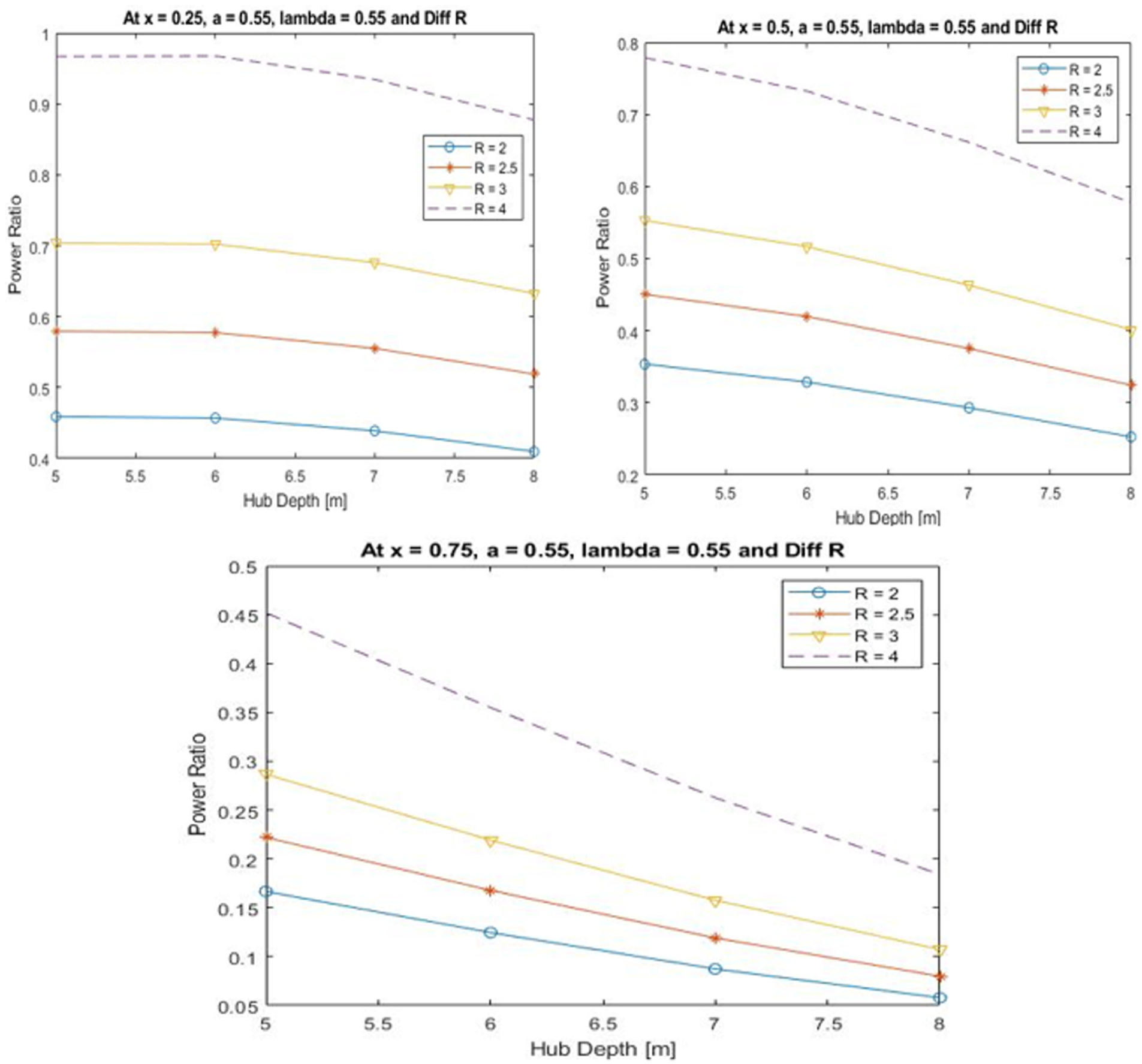
Power ratio versus hub depth (m) at alpha = 0.55, Lambda = 0.55, (Diff R (m)).

Figure 8 illustrates the relationship between the tidal turbine power ratio and the free flow velocity U at a constant wavelength (λ = 0.55 m) and hub depth (Hb = 5 m). The results reveal a clear positive proportionality between the power ratio and the flow velocity within the examined range. As shown, the maximum power ratio of 0.95 occurs at a velocity of 14 m/s for the horizontal position x = 0.25, while the minimum power ratio of 0.48 is observed at 5 m/s for the same wave amplitude model. This strong dependence on velocity arises because the power extracted by a tidal turbine is governed by the cubic relationship P = 12ρACpU³, where A is the rotor swept area, ρ is the water density, and Cp is the power coefficient. Therefore, even a small increase in velocity leads to a substantial rise in the available kinetic energy and, consequently, in the generated power. At the horizontal position x = 0.75 and wave amplitude of 0.75 m, the same pattern is observed: when the free flow velocity reaches 14 m/s, the power ratio attains approximately 0.6, while it drops below 0.3 at 5 m/s. Physically, this behavior can be explained by the higher momentum flux and energy density in the faster flow regime. As velocity increases, the fluid’s dynamic pressure and inertial forces acting on the turbine blades intensify, producing greater torque and mechanical power output. Conversely, at lower velocities, both the kinetic energy and turbulence intensity diminish, reducing the momentum exchange between the flow and the rotor blades and hence the power ratio.

Figure 8.

Power ratio versus free flow velocity (m/s) at Lambda = 0.55, (Hb = 5 m, R = 4 m).

For the wave amplitude reached to 0.55, horizontal position = 0.25, and the hub Depth = 5 m, a large verified power ratio will be valid at wave length = 0.55 at 14 m/s flow speed, reached 0.96, whereas the power ratio decays to a half, 0.47 when the flow speed cut to 5 m/s for the same wave length. The noted power ratio gives drops as the wave length increases, as illustrated in Figure 9. The generated power ratio is proportional with increasing Free Flow Velocity and inversely proportional with wave length. At x = 0.75 and wavelength = 0.55, the power ratio for the model could be vary from 0.25 to a grown value success to 0.59 when the free flow velocity rises from 5 to 14 m/s, decreasing wave length will enhance the amount of the produced power in wide range of the Free Flow Velocity.

Figure 9.

Power ratio versus free flow velocity (m/s) at alpha = 0.55, (Hb = 5 m, R = 4 m).

As Figure 10 presents, four models with radius = 4 m, at horizontal position, x = 0.25, and wavelength = 0.55. The output power increase as flow turbulence intensity increase. Increasing of turbulence intensity (b) means increasing of the inertia forces of fluid layers attacking turbine blades, which leads to increase the generated power of the tidal turbine. At x = 0.5, the relation between the output power and the flow turbulence is proportional for the wave amplitude begun from 0.55 to 0.75, changing from 0.25 to 0.85 in the range of 31,000–100,000 flow turbulence. This result demonstrates the increasing of turbulence intensity (b) leads to increase the eddy viscosity and indicate increasing in the inertia forces of fluid layers which are attacking turbine blades, leads to increasing in the generated power. In addition to that, when the value of wave amplitude increase, the value of velocity increases as well as the generated power ratio.

Figure 10.

Power ratio versus turbulence intensity (b) at Lambda = 0.55, R = 4 m.

Figure 11 presents the mesh dependency analysis for the finite-element model by showing how the predicted power ratio responds to successive mesh refinements. The trend follows the expected convergence pattern. With a coarse mesh of approximately 50 elements, the predicted power ratio is 0.48. Refining the mesh to 100 elements increases the power ratio to 0.53, reflecting the reduction in discretization error and improved resolution of flow gradients around the turbine blades. Further refinement to 200 elements yields a more modest rise to 0.54, and increasing the mesh to 250 elements produces only a negligible change, reaching a final power ratio of 0.55. The flattening of the curve at higher mesh densities indicates that the numerical solution has reached mesh independence: beyond approximately 200 elements, additional refinement no longer produces meaningful variation in the output.

Figure 11.

Mesh independence study for the proposed model (power ratios vs number of elements).

Validation and comparison

The simulated power ratios obtained in this study were validated against several published experimental and numerical investigations. Our baseline case (Power ratio = 0.55) aligns well with Ghamati et al., ⁹ whose maximum Cp = 0.52, confirming consistency in the order of magnitude. Wave–current interaction cases showed increases up to ∼20%–40%, comparable to the ±45% variations reported by Min et al. ¹⁰ for free-surface exposure effects. Turbulence sensitivity tests reproduced the 5%–15% performance shifts observed by Mycek et al. ¹¹ and Pinon and Rivoalen, ¹² indicating correct response to inflow variability. Similarly, wave-induced wake alterations ¹³ matched our simulated trends of enhanced near-surface power and accelerated wake recovery. Comparison with full-scale and field data^14,15 showed that our normalized Power Ratio remains within the realistic performance envelope of Cp = 0.29–0.43. Moreover, CFD benchmarks under unsteady inflow ¹⁶ demonstrated similar power reductions (∼5%) to those found in our unsteady cases. Overall, the agreement across diverse studies confirms the reliability and physical validity of the developed model.

Conclusion

A theoretical and numerical model was developed in MATLAB^© to investigate tidal turbine performance under wavy flow conditions based on continuity, momentum, and turbine power equations. The model examined the effects of wave amplitude, wavelength, rotor radius, hub depth, and free flow velocity on turbine power ratio.

The results showed that the optimal operating condition occurs at a hub depth of 5 m, rotor radius of 4 m, wave amplitude of 0.55 m, and wavelength of 0.55 m, yielding a maximum power ratio of 0.97. Reducing the rotor radius to 2 m under the same conditions decreases the power ratio to 0.46, due to the smaller swept area and reduced energy capture. Similarly, increasing the hub depth from 5 to 9 m led to a drop in power ratio from 0.88 to 0.41, confirming that deeper installations encounter lower flow velocities.

For variations in free flow velocity, the power ratio increased from 0.48 at $5\mathrm{m}/\mathrm{s}$ to 0.95 at $14\mathrm{m}/\mathrm{s}$ for $x=$ 0.25, and from 0.3 to 0.6 for $x=0.75$ . This trend validates the cubic dependence of turbine power on flow velocity. Shorter wavelengths (e.g., 0.55 m) produced significantly higher power output compared to longer ones (e.g., 0.65 m), emphasizing the role of increased flow acceleration and turbulence.

Overall, the findings confirm that larger rotor radii, higher wave amplitudes, shorter wavelengths, and shallower hub depths yield higher energy output. These quantitative results provide valuable insight for optimizing the design and placement of tidal turbines to maximize energy extraction efficiency.

The following are the main conclusions reached as a result of this study:

1. Wavelength (Lambda), wave amplitude (a), detect the optimal values of the wavy flow that are able to control the possibly generated output power of the Tidal turbine. As shown in the study, when Lambda decreases the power of the turbine increase. However, the output power increases with the increase of wave amplitude.

2. Increasing Turbine Rotor Radius (R) and Hub Depth (Hb) influences directly on the output power; Turbine Radius (R) rises the amount of captured flowing fluid meaning more hydropower.

3. As illustrated in the study, the produced power decreases as the Hub Depth increases in turbulent flow.

4. The tidal turbine produced power would increase with the increase of turbulence intensity. The reason of this result is due to the increasing the inertia forces of fluid layers attacking turbine blades.