Sage Journals: Discover world-class research

Abstract

Giant magnetostrictive actuators (GMAs) usually have the problem of significant temperature change caused by power losses under pulse width modulation (PWM) excitation. It leads to thermal deformation and a decrease in the magnetostriction coefficient, which degrades their performance of position control. This paper introduces a novel dual-flow-channel (DFC) cooling structure that includes outer and inner flow channels. Flow grooves are machined into the magnetic sleeve to form the outer flow channel in conjunction with the shell, while the inner flow channel immerses the giant magnetostrictive material (GMM) rod. DFC cooling structure achieves efficient heat dissipation for GMA while preserving its original volume and maintaining good sealing. A thermal analytical model of GMA, based on the lumped-parameter thermal network (LPTN), is employed to achieve rapid and accurate prediction of thermal characteristics. Based on the Jordan loss model, the GMM loss model under sinusoidal excitation was improved to develop a GMM loss model under PWM excitation. A prototype of GMA was designed and machined, and its thermal characteristics were tested. The experimental results show that, under ambient conditions of 20 °C, with a current amplitude of 5 A, a PWM frequency of 50 Hz, and a coolant flow rate of 0.5 L/min, the final temperature of the GMA with the DFC cooling structure decreased from 45 °C to 23.5 °CC. The relative errors between the analytical and experimental results were <11% under different conditions, validating the accuracy of the proposed analytical model. This study provides important theoretical support for the investigation of thermal deformation in GMAs under PWM excitation.

Keywords

GMA cooling structure thermal network model loss model LPTN

Introduction

As a kind of smart material, GMM has the characteristics of high magnetostriction, large output force, and rapid response.^1–5 It shows strong development potential in electro-hydraulic servo control systems, particularly in driving high-speed switching valves.^6–12 However, high-speed switching causes the GMM rod and coil to generate excessive heat, leading to a significant temperature change in GMA. The compact structure of GMA further exacerbates the temperature change.^13,14 This results in thermal deformation of the GMM rod and a decrease in the magnetostriction coefficient, both of which negatively influence the accuracy of precise position control. Therefore, appropriate cooling measures must be taken to maintain stable operating temperatures.

Many researchers are working on the cooling structure of GMA. Ji et al. developed a pipe cooling structure with pipes wrapped around the GMM rod and coil, which effectively dissipated heat but increased the complexity and volume of GMA.¹⁵ Cui et al. proposed an inner chamber cooling structure positioned between the coil and the GMM rod, yet they ignored the impact of the thermal deformation of other components on output displacement.¹⁶ Ju et al. designed a GMA with its coil immersed in cooling oil completely, and a rubber tube was installed at the oil inlet to ensure proper circulation, yet they ignored the heat generated by the GMM rod.¹⁷ Lu et al. proposed a dual inner and outer chamber cooling structure for GMA and developed a water-cooling temperature control system.¹⁸ Experiments demonstrated improved heat dissipation, yet no further detailed study on the cooling structure was conducted, and the cooling structure increased the volume of GMA. Electro-hydraulic servo devices using GMAs as the electro-mechanical converters can naturally use hydraulic oil as a cooling medium. Li et al. designed a GMA with a hollow-structured GMM rod as a valve actuator, where the hollow structure serves as a flow channel for cooling.¹⁹ Wang et al. proposed a method that utilized the leakage oil from a nozzle-flapper valve as the cooling medium for GMA to reduce thermal deformation, and verified the effectiveness of this method through experiments conducted at different ambient temperatures.²⁰ However, long-term operation of hydraulic systems may produce contaminants in the oil to wear the surface insulation of the coil, leading to short circuits. Therefore, when hydraulic oil is regarded as the cooling medium, the coil must be isolated from the oil for electric safety. In summary, while the above cooling structures offer effective heat dissipations, they also increase the size and complexity of GMAs, even the risk to electric safety, highlighting the need for compact integration and reliable sealing.

To address these issues, engineers at Lucid Group, Inc. introduced cooling channels into areas of the stator of a permanent magnet synchronous motor (PMSM) where there is no magnetic flux distribution. This method establishes a novel cooling system that enhances motor efficiency without increasing its volume, while the coil is isolated from the cooling fluid.²¹ The magnetic sleeve of GMA is similar to the stator of PMSM, and cooling channels can be established on the magnetic sleeve. However, unlike the laminated silicon steel sheets of PMSM, the magnetic sleeve of GMA is manufactured integrally, making it demanding to drill holes in its thin and long axial structure.

Besides, electromagnetics, thermodynamics, and fluid mechanics are often integrated into the analytical modeling of the GMA cooling structure, which makes the modeling process complex and challenging.^22,23 As a result, researchers often rely on computer-aided design (CAD) techniques.^15,19 Although CAD provides numerical results in detail, it demands high computational time costs for iterative calculations and makes targeted optimization difficult. In contrast, analytical modeling offers a fast and accurate method for calculating the thermal characteristics of GMA once formulated as an explicit expression. It provides essential theoretical support for thermal management and cooling structure optimization. For instance, Deng et al. developed a thermal analytical model for the pipe cooling structure to investigate the relationship between the thermal characteristics of GMA and flow rate.²³ Furthermore, Zhu and Ji combined thermal compensation and an inner cooling chamber, and established an analytical model that reveals the relationship between the output characteristics of GMA and the combined cooling structure.²⁴ However, thermal analytical models of the proposed dual inner and outer chambers cooling structure have not yet been reported yet, which is necessary for its thermal characteristic prediction and future optimization.

Finally, the drive signal for GMA is primarily a PWM signal when driving high-speed switching valves.¹¹ However, there is very limited research on core loss in GMM under PWM excitation, as most GMM loss models are based on sinusoidal excitation.^24,25 It is important to highlight that core losses vary considerably between these two types of excitations, making it unreliable to apply sinusoidal-based loss models to the thermal modeling under PWM excitation.²⁶ Therefore, it is necessary to study the GMM loss model under PWM excitation, which is another highlight of this research. Moreover, the thermal analytical model proposed in this paper treats the coolant flow rate, current amplitude, and excitation frequency as independent and variable input parameters. This significantly enhances its practical relevance for engineering applications. In contrast, the thermal analytical models in the aforementioned literature usually assume either constant cooling conditions or constant input power, which lacks a comprehensive consideration of both thermal boundary conditions and input excitation.

This paper introduces a novel dual-flow-channel (DFC) cooling structure for GMA, which includes the outer and inner flow channels. Flow grooves are machined into the magnetic sleeve to form the outer flow channel in conjunction with the shell, while the GMM rod is immersed in the inner flow channel. The corresponding GMA thermal analytical model under PWM excitation is also employed for predicting the temperature of GMA, which is necessary for thermal characteristic prediction and future optimization of the DFC cooling structure.

The rest of this paper is organized as follows: In Section 2, the structure of GMA with DFC cooling structure is introduced. In Section 3, a thermal analytical model of GMA based on LPTN is employed, and a GMA loss model under PWM excitation is built. In Section 4, the prototype of GMA is designed and machined, and its thermal characteristics are tested with an experimental platform. In Section 5, a comprehensive summary of the above work is provided.

Structure of GMA

GMA consists of a GMM rod, coil components, magnetic components, shell components, preload components, an output shaft, and several O-rings, as shown in Figure 1. The coil components are arranged inside the magnetic sleeve and generate a magnetic field around the GMM rod when energized. The magnetic components include the magnetic cap, magnetic cylinder 1, magnetic cylinder 2, and magnetic sleeve, all of which form the magnetic circuit with the GMM rod to ensure the magnetostriction performance. The shell components include the shell, front, and rear end caps. The preload components include a preload screw and disc springs, which apply pre-tension to the GMM rod to enhance the magnetostriction performance.

Figure 1.

Schematic diagram of GMA structure.

In Figure 1, the green line represents the flow channel of DFC cooling structure, and the green arrow represents the flow direction. The proposed DFC cooling structure includes the outer flow channel and the inner flow channel.

The inlet and outlet of the flow channels are located on the shell. The axial flow grooves are uniformly distributed along the surface of the magnetic sleeve, while the circumferential flow grooves are located on both sides. After entering through the inlet, the cooling oil in the outer flow channel first flows into the left circumferential flow groove. It then passes through the middle axial flow groove and the right circumferential flow groove before exiting through the outlet. These flow channels and grooves form the outer flow channel. The coil holder is thickened on both sides to accommodate two radial flow channels. The cooling oil in the inner flow channel enters through the inlet, flows first through the left radial flow channel, then moves into the annular space between the GMM rod and coil holder, and flows along the axial direction. Afterward, it flows through the right radial flow channel and exits through the outlet. These flow channels form the inner flow channel. The inner and outer flow channels surround the coil to dissipate its heat, and the inner flow channel also dissipates the heat from the GMM rod.

The fluid domain of DFC cooling structure is illustrated in Figure 2(a). Computational fluid dynamics (CFD) is used to visualize the fluid flow within the cooling structure, and the result is shown in Figure 2(b). It is evident that the fluid particles follow the described paths through both the inner and outer flow channels.

Figure 2.

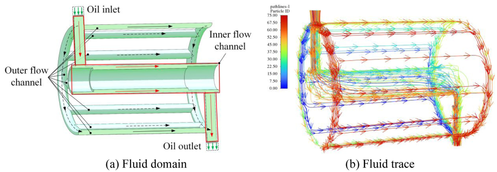
Schematic diagram of DFC cooling structure: (a) fluid domain and (b) fluid trace.

Analytical model

LTPN method

The advancement of CAD technologies has made CFD an essential tool for thermal analysis in electric machines. However, due to its high computational time costs, CFD is not suitable for the preliminary design of electrical machines. To address this issue, this paper employs LPTN to develop a thermal network model of GMA for thermal analysis. Figure 3 illustrates the flowchart of the GMA thermal network modeling process.

Figure 3.

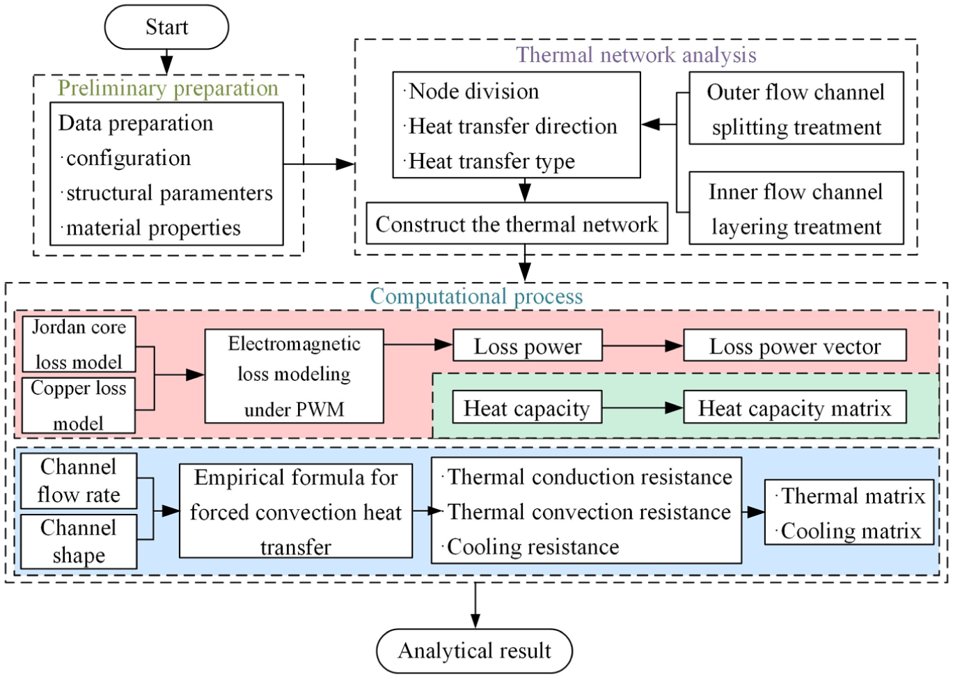
Flow chart of the GMA thermal network modeling.

To facilitate computation and improve accuracy, the following assumptions are adopted:

The temperature distribution is symmetric about the axis.

Thermal capacity and heat generation of each node are uniformly distributed.

Heat transfers in the radial and axial directions are independent.

Node division

Most components of GMA are cylindrical and have rectangular radial cross-sections. Therefore, node division is applied to the radial cross-sections. Specifically, the GMA is divided into 43 mesh elements, with the center of each element serving as a node. It is assumed that the temperature distribution within each mesh element is uniform. To improve the accuracy of the analytical model, the GMM rod and other components with certain axial lengths are further axially divided into multiple elements. The schematic of node division is shown in Figure 4.

Figure 4.

Schematic diagram of node division for GMA.

Among the 43 element nodes, nodes 8–12 and 28–37 are fluid element nodes, while the remaining nodes are solid element nodes. The thermal interactions between fluid and solid element nodes require optimization for subsequent calculations.

To illustrate the thermal interactions and optimizations in the inner and outer flow channels, the cross-section of nodes 4–39 is selected as an example. The outer flow channel is in contact with both the shell and the magnetic sleeve, where thermal convection occurs between the outer flow channel node 9 and the shell node 4, and between node 9 and the magnetic sleeve node 15. Additionally, the magnetic sleeve is in direct contact with the shell, where thermal conduction occurs between nodes 4 and 15. To accurately model these thermal interactions, nodes 4 and 15 are subdivided into three sub-nodes each.

As shown in Figure 5(a), the heat transfer between the shell and the magnetic sleeve is handled by the sub-nodes on either side. Meanwhile, the central sub-node is responsible for the heat transfer between the shell and the outer flow channel, as well as between the magnetic sleeve and the outer flow channel. Furthermore, it is assumed that there is no temperature difference between the sub-nodes. Therefore, the three sub-nodes are combined into a single parent node for simplicity, as shown in Figure 4.

Figure 5.

Schematic diagram of node optimization treatment for flow channels: (a) outer flow channel splitting treatment and (b) inner flow channel layering treatment.

For the inner flow channel, the temperature field of thermal convection can be divided into the thermal boundary layer and the mainstream layer. As shown in Figure 6, the orange arrows represent the intensity of thermal convection, with larger arrows indicating stronger convection in that region. The blue arrows represent the direction of fluid flow, with larger arrows corresponding to higher flow velocities.

Figure 6.

Layering principle of the inner flow channel.

In the mainstream layer, the temperature change of the fluid is minimal, while the thermal boundary layer exhibits a significant temperature gradient. The heat sources of the inner and outer layers are the GMM rod and the coil, respectively. Due to their different heat generation powers, the rate of temperature changes in the thermal boundary layers differs significantly. Consequently, it is inappropriate to directly apply the Nu empirical formulas for thermal convection in annular spaces. Instead, the inner flow channel should be optimized by dividing it into two radial layers, with the mainstream layer at the center. Given that the temperature change in the mainstream layer is negligible, the outer wall of the inner layer nodes and the inner wall of the outer layer nodes can be assumed to have an adiabatic boundary.

Therefore, as shown in Figure 5(b), the inner flow channel is divided into outer layer node 29 and inner layer node 34. The outer layer is in contact with the coil holder, leading to thermal convection between coil holder nodes 25 and 29. The inner layer is in contact with the GMM rod, resulting in thermal convection between node 34 and the GMM rod node 39. There is no heat transfer between nodes 29 and 34, as they are separated by the mainstream layer.

In summary, the thermal network of GMA is illustrated in Figure 7. Since the oil temperature is lower than that of the solid components, the oil acts as a heat sink. To indicate the unidirectional heat transfer from the solid components to the oil, a diode symbol is incorporated into the heat transfer path between them. Finally, the material properties for each node are provided in Table 1.

Figure 7.

Schematic diagram of LPTN thermal network model.

Table 1.

Node material properties.

Node	Material	Specific heat capacity, c (J/(kg K))	Heat conductivity, k (W/(m K))	Density, ρ (kg/m³)
1–7, 19, 23, 25–27, 43	Al alloy 6061	896	180	2719
8–12, 28–37	46# Hydraulic oil	1955	0.144	850
13–18, 24 38, 42	DT4C	574	54.7	7870
20–22	Coil	381	387.6	8978
39–41	GMM	330	13.5	9250

Loss model under PWM

PWM wave is used as the excitation signal when GMA drives a high-speed switching valve. This excitation method facilitates efficient power conversion and precise position control. However, compared to traditional sinusoidal wave, the loss under PWM excitation exhibits significantly different loss characteristics. To ensure the accuracy of the analytical model, it is essential to re-evaluate the loss of GMA under PWM excitation.

Copper loss

Due to the frequency multiplication characteristics of GMM, GMA requires a signal with a DC bias as the excitation signal.¹¹ Based on a DC-biased square wave, the formula for calculating the copper loss in GMA under PWM excitation is:

P_{copperloss} = {[\sqrt{{DI}_{He}^{2} + (1 - D) I_{Le}^{2}}]}^{2} R_{coil}

(1)

Where D is the duty cycle; I_He is the effective current during the high-level period; I_Le is the effective current during the low-level period; R_coil is the resistance of the coil.

Core loss

Based on the mechanisms of core loss, the losses under sinusoidal excitation can be decomposed into three components: hysteresis loss, eddy current loss, and residual loss.²⁷ Under high-frequency excitation, eddy current loss becomes dominant, and the residual loss caused by the bending of magnetic domain walls can be neglected.^28,29 Thus, the three-term loss separation model can be simplified to the Jordan model, which is expressed as:

P_{\sin} = P_{h} + P_{e} = k_{h} B_{m}^{β} f + k_{e} B_{m}^{2} f^{2}

(2)

Where k_h and k_e are the hysteresis loss coefficient and the eddy current loss coefficient, respectively.

The hysteresis loss within a single cycle is mainly influenced by the peak magnetic flux density, irrespective of the excitation waveform. Therefore, when the peak magnetic flux density is equal, the hysteresis loss under DC-biased square wave excitation is only half of that under sinusoidal wave excitation. The eddy current loss under DC-biased square wave excitation can be expressed as the product of two components. The first component is the eddy current loss under sinusoidal wave excitation. The second component is the waveform factor α, which is defined as the ratio of the area enclosed by the non-sinusoidal magnetic flux density waveform and the t-axis to that of the sinusoidal waveform (Figure 8).³⁰

Figure 8.

Voltage and magnetic density waveforms under sinusoidal and DC-biased square wave excitation: (a) voltage waveforms and (b) magnetic density waveforms.

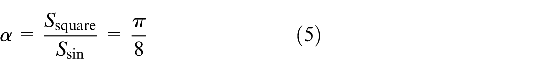
The area enclosed by the magnetic flux density waveform and the t-axis under the sinusoidal wave is:

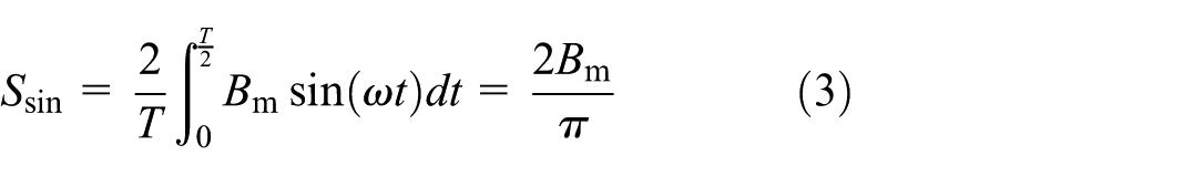
S_{\sin} = \frac{2}{T} \int_{0}^{\frac{T}{2}} B_{m} \sin (ω t) dt = \frac{2 B_{m}}{π}

(3)

The area enclosed by the magnetic flux density waveform and the t-axis under the DC-biased square wave is:

S_{square} = \frac{2}{T} \int_{0}^{\frac{T}{4}} \frac{B_{m}}{T / 4} dt = \frac{B_{m}}{4}

(4)

From equations (3) and (4), the waveform factor α under DC-biased square wave can be obtained:

α = \frac{S_{square}}{S_{\sin}} = \frac{π}{8}

(5)

From the above expressions, the core loss under the DC-biased square wave is:

\begin{matrix} P_{square} = \frac{1}{2} P_{h} + α P_{e} \\ = \frac{1}{2} k_{h} B_{m}^{β} f + \frac{π}{8} k_{e} B_{m}^{2} f^{2} \end{matrix}

(6)

Referring to the magnetic flux density-power loss (B–P) curve in Huang et al.,³¹ the expression of iron loss calculation is fitted with k_h = 7.55, k_e = 4.63 × 10⁻⁴, β = 2.³¹ The B–P curve for GMM under the DC-biased square wave is shown in Figure 9.

Figure 9.

B–P curve of GMM under DC biased square wave excitation.

The equivalent magnetic circuit of GMA is as shown in Figure 10. Here Ni is the magnetomotive force of the coil; ϕ is the magnetic flux; R_mc1, R_me, R_ms, R_mc2, and R_GMM are the magnetic reluctances of the magnetic cylinder 1, magnetic cap, magnetic sleeve, magnetic cylinder 2, and GMM rod, respectively; R_m1 is the leakage reluctance of the coil, which is connected in parallel with the coil.³²

Figure 10.

Equivalent magnetic circuit for GMA.

The expression for magnetic flux is:

ϕ = γ ϕ_{1}

(7)

Where γ is the leakage flux coefficient, taken as 0.75; ϕ₁ is the total magnetic flux generated by the coil.

The leakage flux coefficient γ is obtained through electromagnetic field simulation. It is the ratio of the number of effective magnetic flux lines to the total number of magnetic flux lines.

According to Kirchhoff’s law, the closed-loop magnetic flux relationship is:

Ni = ϕ (R_{mc 1} + R_{me} + R_{ms} + R_{mc 2}) + ϕ_{1} R_{GMM}

(8)

Where the value of relative permeability for GMM is taken as 6.³³

The magnetic flux density B_m at the GMM rod is shown in equation (9). By substituting equation (9) into equation (6), the power loss of the GMM rod is obtained.

B_{m} = \frac{ϕ_{1}}{A_{GMM}}

(9)

Where A_GMM is the cross-sectional area of the GMM rod.

The magnetic density calculated using equation (9) is compared with the Maxwell simulated results, as illustrated in Figure 11. It can be seen that the relative error between the analytical and simulated results is <10% from 3 to 5 A, which verifies the accuracy of magnetic circuit model.

Figure 11.

Magnetic density at GMM for different currents.

Thermal conduction matrix

Thermal matrix

The thermal matrix is:

G = (\begin{matrix} \sum_{1}^{n} \frac{1}{R_{1, i}} & - \frac{1}{R_{1, 2}} & \dots & - \frac{1}{R_{1, n}} \\ - \frac{1}{R_{2, 1}} & \sum_{1}^{n} \frac{1}{R_{2, i}} & \dots & - \frac{1}{R_{2, n}} \\ ⋮ & ⋮ & ⋱ & - \frac{1}{R_{3, n}} \\ - \frac{1}{R_{n, 1}} & - \frac{1}{R_{n, 2}} & \dots & \sum_{1}^{n} \frac{1}{R_{n, i}} \end{matrix})

(10)

Where R_ij is the thermal resistance between nodes i and j; R_ij = R_ji, representing the feedback between nodes; the diagonal elements represent the sum of thermal conductivities connected to node i.

In the GMA thermal model, thermal resistances are mainly divided into thermal conduction and thermal convection type. The thermal resistances associated with nodes 14–18 or nodes 28–37 are a combination of thermal convection and thermal conduction type, while the remaining thermal resistances are purely thermal conduction type.

According to the schematic diagram of node division shown in Figure 4, the heat transfer directions for thermal conduction are primarily axial and radial, and their thermal resistance models are shown in Figure 12.

Figure 12.

Thermal resistance models: (a) axial heat transfer and (b) radial heat transfer.

The thermal resistance for axial and radial heat transfer are:

{\begin{matrix} R_{axial} = \frac{l_{1}}{k_{1} A} + \frac{l_{2}}{k_{2} A} \\ R_{radial} = \frac{\ln \frac{r_{1}}{r_{2}}}{2 π k_{1} l_{3}} + \frac{\ln \frac{r_{2}}{r_{3}}}{2 π k_{2} l_{3}} \end{matrix}

(11)

Where k₁ and k₂ are the thermal conductivities of materials 1 and 2, respectively; l₁ and l₂ are the axial lengths between nodes i and j; A is the contact area between the mesh elements of nodes i and j; r₁, r₃, and r₂ represent the radius of the circumferential surfaces of nodes i and j, and the contact surface between their mesh elements, respectively; l₃ is the contact length between the mesh elements of nodes i and j.

Thermal convection resistance

The equations for thermal convection resistance are:

{\begin{matrix} R = \frac{l_{4}}{h_{c} A} \\ h_{c} = \frac{Nu k_{fluid}}{d_{e}} \end{matrix}

(12)

Where l₄ is the contact length between nodes; A is the contact area; h_c is the convective heat transfer coefficient;

Nu is the Nusselt number; k_fluid is the thermal conductivity of the fluid; d_e is the equivalent diameter of the node element.

The thermal convection in the inner and outer flow channels of GMA belongs to laminar forced convection inside pipes and grooves, which is well-studied, and there is a wealth of established results available for reference (Tao).³⁴ For the outer flow channel, the Sieder–Tate formula is used, along with its applicable conditions are:

{\begin{matrix} N u_{out} = 1.86 {(\frac{Re ⪻}{l / d_{e}})}^{1 / 3} {(\frac{η_{f}}{η_{w}})}^{0.14} \\ ⪻ = 0.48 ~ 16700 \\ \frac{η_{f}}{η_{w}} = 0.0044 ~ 9.75 \\ {(\frac{RePr}{l / d})}^{\frac{1}{3}} {(\frac{η_{f}}{η_{w}})}^{0.14} \geq 2 \end{matrix}

(13)

Where Re is the Reynolds number; Pr is the Prandtl number; l is the axial length; d_e is the equivalent diameter; η_f is the viscosity of the oil at fluid temperature; η_w is the viscosity of the oil at wall temperature.

In the design of the outer flow channel, two key parameters are the number of flow channels n and the radius r of the flow channels. To achieve efficient cooling, the primary objective is to minimize thermal resistance. Therefore, it is crucial to analyze the relationship among n, r, and the resulting thermal resistance. This analysis will help optimizing the cooling efficiency of GMA.

The cross-section of the outer flow channel is unfolded along the circumferential plane, as shown in Figure 13. Due to the complexity of calculating the angle θ of the flow channel cross-section, it is as ∼180° for simplicity.

Figure 13.

Schematic diagram of unfolded outer flow channel.

The cross-sectional area A_e, wetted perimeter l_e, and the contact area A between the outer flow channel and the magnetic sleeve are:

{\begin{matrix} A_{e} = \frac{π r^{2}}{2} \\ l_{e} = π r + 2 r \\ A = π nlr \end{matrix}

(14)

The equivalent hydraulic diameter d_e of the outer flow channel cross-section is calculated.

d_{e} = \frac{4 A_{e}}{l_{e}}

(15)

The total cross-sectional area A_out of the outer flow channel is:

A_{out} = n A_{e}

(16)

The flow rate in the outer flow channel is calculated as:

{\begin{matrix} Q = A_{out} u_{1} + A_{in} u_{2} \\ \frac{u_{1}}{u_{2}} = \frac{A_{in}}{A_{out}} \\ u_{1} = \frac{Q}{2 A_{out}} \end{matrix}

(17)

Where Q is the total fluid flow rate; A_in is the cross-sectional area of the inner flow channel; u₁ is the flow velocity in the outer flow channel; u₂ is the flow velocity in the inner flow channel.

Substituting the equations (14), (15), (17) to (21), (23) into equation (13) for derivation, it yields:

\begin{matrix} R = \frac{l}{h_{c} A} = \frac{l}{\frac{N u_{out} \cdot k}{d_{e}} A} = \frac{l^{\frac{4}{3}}}{1.86 k ⪻^{\frac{1}{3}} (\frac{η_{f}}{η_{w}})} \frac{d_{e}^{\frac{2}{3}}}{AR e^{\frac{1}{3}}} \\ = ε_{1} \frac{d_{e}^{\frac{2}{3}}}{AR e^{\frac{1}{3}}} = ε_{2} \frac{d_{e}^{\frac{1}{3}}}{n \cdot r \cdot u^{\frac{1}{3}}} = ε_{3} \cdot \frac{1}{n \cdot r^{\frac{2}{3}} \cdot u^{\frac{1}{3}}} \\ = ε_{4} \cdot n^{- \frac{2}{3}} \end{matrix}

(18)

Where:

{\begin{matrix} ε_{1} = \frac{l^{\frac{4}{3}}}{1.86 kP r^{\frac{1}{3}} (\frac{η_{f}}{η_{w}})} \\ ε_{2} = ε_{1} \frac{ν_{f}^{\frac{1}{3}}}{π l} \\ ε_{3} = ε_{2} \cdot (\frac{4 π}{π + 2})^{\frac{1}{3}} \\ ε_{4} = ε_{3} \cdot {(\frac{π}{Q})}^{\frac{1}{3}} \end{matrix}

(19)

After establishing the qualitative relationship among n, r, and thermal resistance, it is evident that the cooling effectiveness of the outer flow channel depends solely on the number of flow channels n.

The inner flow channel is divided into the outer and inner layers. The outer layer features an adiabatic inner wall, while the inner layer features an adiabatic outer wall. The value of Nu for these nodes can be taken from Table 2.

Table 2.

Nu for laminar heat transfer in an annular space.³⁴

Ratio of inner to outer diameter, d_i/d_o	Inner wall Nu_i with adiabatic outer wall	Outer wall Nu_o with adiabatic inner wall
0	/	3.66
0.05	17.46	4.06
0.10	11.56	4.11
0.25	7.37	4.23
0.50	5.74	4.43
1.00	4.86	4.86

Cooling matrix

The calculation methods for the cooling matrix and cooling resistance are as follows. Unlike the thermal matrix, the cooling fluid flows unidirectionally in the flow channels, so there is no feedback between nodes, making the cooling matrix a triangular matrix.³⁵

G_{fluid} = (\begin{matrix} \sum_{1}^{n} \frac{1}{R_{q 1 i}} & - \frac{1}{R_{q 12}} & \dots & - \frac{1}{R_{q 1 n}} \\ 0 & \sum_{1}^{n} \frac{1}{R_{q 2 i}} & \dots & - \frac{1}{R_{q 2 n}} \\ ⋮ & ⋮ & ⋱ & - \frac{1}{R_{q 3 n}} \\ 0 & 0 & \dots & \sum_{1}^{n} \frac{1}{R_{qni}} \end{matrix})

(20)

R_{q} = \frac{1}{ρ_{mass} q_{V} c_{p}}

(21)

Where R_qii is the thermal resistance of the cooling fluid flowing through node I; R_qij is the thermal resistance of the cooling fluid flowing from node i to node j; ρ_mass is the mass density of the cooling fluid; q_V is the volumetric flow rate of the cooling fluid; c_p is the specific heat capacity of the cooling fluid.

Heat capacity matrix

The calculation for the heat capacity matrix C and the heat capacity C_i of node i can be expressed as:

C = [\begin{matrix} C_{1} & 0 & \dots & 0 \\ 0 & C_{2} & \dots & 0 \\ ⋮ & ⋮ & ⋱ & ⋮ \\ 0 & 0 & \dots & C_{i} \end{matrix}]

(22)

C_{i} = m_{i} c_{i}

(23)

Where C_i is the heat capacity of node i; m_i is the mass of node i; c_i is the specific heat capacity of the material at node i.

Analytical results

The calculation expressions for steady-state and transient thermal characteristics of GMA are shown in equations (24) and (25), respectively.

Δ T = (G + G_{fluid})^{- 1} P

(24)

\frac{d (Δ T)}{dt} = C^{- 1} P - C^{- 1} (G + G_{fluid}) Δ T

(25)

Where ΔT is the matrix of temperatures relative to the reference temperature for each node; G is the thermal matrix; G_fluid is the cooling matrix; P is the vector of loss power for each node.

The structural parameters are listed in Table 3. These parameters are substituted into the analytical model, whose results are compared with simulated results.

Table 3.

Structural parameters of GMA.

Parameter (unit)	Value
Outer diameter of the GMM rod (mm)	10
Length of the GMM rod (mm)	50
Outer diameter of the coil (mm)	45
Inner diameter of the coil (mm)	18
Length of the coil (mm)	55
Inner diameter of the coil holder (mm)	14
Length of the coil holder (mm)	77
Thickness of shell (mm)	4.5
Diameter of the output shaft (mm)	4
Length of the output shaft (mm)	36
Outer diameter of the outer flow channel (mm)	55
Radius of cross-section of the outer flow channel groove (mm)	2.5
Number of the outer flow channels	12
Length of the outer flow channel (mm)	73
Outer diameter of the inner flow channel (mm)	14
Thickness of the magnetic cap (mm)	4
Thickness of the bottom of magnetic sleeve (mm)	4
Diameter of the magnetic cylinders (mm)	6
Length of the magnetic cylinder 1 (mm)	15
Length of the magnetic cylinder 2 (mm)	20

Figure 14 illustrates the analytical and simulated results for the thermal characteristics of GMA at 5 A current amplitude, 50 Hz PWM, and a flow rate of 0.5 L/min. The initial temperature is 20 °C, and the final temperatures of the shell, coil, and GMM rod remain below 23.5 °C. The temperature of the GMM rod rises more rapidly owing to its higher power loss density. The close agreement between the analytical and simulated curves for these three components validates that the layered treatment of the inner flow channel and the split treatment of the outer flow channel are correct.

Figure 14.

Thermal characteristics of key components in GMA.

Figure 15 illustrates the analytical and simulated results for the thermal characteristics of GMA at various current amplitudes, 50 Hz PWM, and a flow rate of 0.5 L/min. As the current amplitude increases, the final temperatures of both the shell and GMM rod rise. The analytical results for the shell are slightly higher than the simulated counterparts, whereas those for the GMM rod are marginally lower. The error between the analytical and simulated results diminishes as the current decreases.

Figure 15.

Thermal characteristics of GMA at different current amplitudes: (a) shell and (b) GMM rod.

Figure 16 illustrates the analytical and simulated results for the thermal characteristics of GMA at various PWM frequencies, 5 A current amplitude, and a flow rate of 0.5 L/min. The temperature of the GMM rod decreases as the PWM frequency decreases, while the temperature of the shell increases. This occurs because a lower frequency reduces the proportion of current rise time in the cycle, thereby increasing effective current and coil losses. Conversely, a higher frequency increases GMM losses, leading to higher temperatures of GMM rod.

Figure 16.

Thermal characteristics of GMA at different PWM frequencies: (a) shell and (b) GMM rod.

Figure 17 illustrates the analytical and simulated results for the thermal characteristics of GMA at various flow rates, 5 A current amplitude, and a PWM frequency of 50 Hz. As the flow rate increases, the final temperature of the shell decreases, while the final temperature of the GMM decreases only slightly. When the simulated results for the GMM rod at 1 and 2 L/min are nearly identical, the analytical results gradually decrease.

Figure 17.

Thermal characteristics of GMA at different flow rates: (a) shell and (b) GMM rod.

Experiment

Prototype of GMA

To validate the reliability of the theoretical analysis, a prototype of GMA was designed and machined, as shown in Figure 18. Figure 18 provides an overview of the components and the whole prototype of GMA, including the oil pipeline connections and temperature sensor interfaces on the shell. To address the non-uniform temperature distribution on the shell and ensure accurate comparisons with analytical and simulated results, three temperature sensors were installed on the shell. These sensors comprehensively capture temperature changes at different points. The temperatures at three positions were averaged to represent the shell temperature in experiments.

Figure 18.

Prototype of GMA: (a) components of GMA and (b) assembled prototype of GMA.

The cooling medium used in the experiment is 46# hydraulic oil, and its detailed physicochemical properties are shown in Table 4.

Table 4.

Physicochemical properties of 46# hydraulic oil.

Parameter (unit)	Value
Specific heat capacity (J/kg K)	1955
Heat conductivity (W/(m K))	0.144
Density (kg/m³)	850
Dynamic viscosity (Pa s)	0.039
Flash point (°C)	180
Freezing point (°C)	−10
Corrosion test: copper, 100 °C, 3H	Qualified
Moisture (%)	0
Water soluble acid base (%)	0

Experimental platform

Figure 19 shows the experimental schematic and setup for investigating the thermal characteristics of GMA. The experimental setup includes the prototype of GMA, a pump station, a signal generator, a power amplifier, a power supply, temperature sensors (PT100), a data acquisition card, a flow meter (K24), a laser displacement sensor (LK-G150), an oscilloscope, and a PC. Temperature sensors are installed on the GMA shell to monitor temperature data.

Figure 19.

Experimental platform for the thermal characteristic of GMA.

The temperature data from the sensors are collected via the data acquisition card and recorded by the PC. The PWM signal generated by the signal generator is amplified by the power amplifier to drive GMA. The laser displacement sensor measures the output displacement of GMA, which is both displayed and recorded by the oscilloscope. The oscilloscope also records the driving current waveform. The pump station supplies a controlled flow rate of cooling oil to GMA, which is monitored by the flow meter.

Experimental result

To ensure the sealing of the GMA cooling structure, no temperature sensors were installed on the GMM rod, Consequently, only the shell temperature was experimentally monitored and recorded.

Figure 20 illustrates the experimental results for the thermal characteristics of GMA at various current amplitudes, both with and without DFC cooling structure. Without DFC cooling structure, the temperature rise is significant, and the final temperature exceeds 45 °C. With DFC cooling structure, the temperature is maintained below 24 °C, and it stabilizes more rapidly. This indicates that DFC cooling structure effectively suppresses the temperature changes of GMA.

Figure 20.

Thermal characteristics of GMA shell at different current amplitudes: (a) without DFC cooling structure and (b) with DFC cooling structure.

Figure 21 illustrates the experimental results for the thermal characteristics of GMA at different PWM frequencies, both with and without DFC cooling structure. As the frequency increases, the final temperature of GMA decreases. Because a lower frequency reduces the ratio of current rise time in the cycle, thereby increasing effective current and coil losses.

Figure 21.

Thermal characteristics of GMA shell at different PWM frequencies: (a) without DFC cooling structure and (b) with DFC cooling structure.

Figure 22 illustrates the analytical, simulated, and experimental results for the thermal characteristics of GMA at different current amplitudes, 50 Hz PWM, and a flow rate of 0.5 L/min. At 5 A, the experimental curve rises more slowly compared to the analytical and simulated curves. However, the final temperature of the experimental curve is higher than that of the analytical and simulated curves, with an absolute error of 0.35 °C. And the relative error of temperature rise is 9.94%. At 4 and 3 A, the experimental curve closely matches the analytical curve, where the absolute errors of final temperature are 0.02 °C and 0.01 °C. The relative errors of temperature rise are 9.76% and 8.70%, respectively.

Figure 22.

Thermal characteristics of GMA at different current amplitudes.

Figure 23 illustrates the analytical, simulated, and experimental results for the thermal characteristics of GMA at different PWM frequencies, 5 A current amplitude, and a flow rate 0.5 L/min. At 10, 25, and 50 Hz, the absolute errors in final temperatures between the experimental and analytical curves are 0.16 °C, 0.26 °C, and 0.34 °C, respectively. The relative errors of temperature rise are 3.30%, 7.10%, and 9.94%, respectively.

Figure 23.

Thermal characteristics of GMA at different PWM frequencies.

Figure 24 illustrates the analytical, simulated, and experimental results for the thermal characteristics of GMA at different flow rates, 5 A current amplitude, and a PWM frequency of 50 Hz. At all three flow rates, the experimental curve rises more slowly compared to the analytical and simulated curves. However, the final experimental temperature is higher than the analytical and simulated results. At 0.5, 1, and 2 L/min, the absolute errors between the experimental and analytical curves are 0.35 °C, 0.16 °C, and 0.23 °C, respectively. The relative errors of temperature rise are 9.94%, 6.56%, and 10.63%, respectively.

Figure 24.

Thermal characteristics of GMA at different flow rates.

Conclusion

In this paper, a novel DFC cooling structure for GMA has been introduced. Experimental results showed that the final temperature of the GMA with DFC cooling structure decreased from 45 °C to 23.5 °C at 5 A current amplitude, 50 Hz PWM excitation, and a flow rate of 0.5 L/min under ambient conditions of 20 °C, demonstrating the effectiveness of this novel cooling structure.

An in-depth study of DFC cooling structure was conducted using LPTN method. A thermal analytical model of DFC cooling structure was employed. The relative errors between the analytical and experimental results are all <11% at different current amplitudes, PWM frequencies, and flow rates, thereby verifying the accuracy of the analytical model.

Based on the Jordan model, the loss model for sinusoidal excitation was improved to reflect PWM excitation. An equivalent magnetic circuit model for GMA was established and a loss model under PWM excitation was deduced, providing theoretical support for the thermal management of GMA during high-speed switching operations.

The influence of the thermal characteristic on thermal deformation of the GMA can be investigated in future work by developing a thermo-mechanical coupled model. Thus, the thermal deformation in the output of GMA and its impact on the accuracy of displacement and dynamic performance can be predicted with this model.

Footnotes

Handling Editor: Chenhui Liang

ORCID iDs

Leidi Wang

Bin Meng

Author contributions

Bin Meng and Leidi Wang were in charge of the whole paper. Bin Meng and Leidi Wang wrote the manuscript. Leidi Wang, Mingzhu Dai, and Yuzhou Huang assisted with sampling and laboratory analyses. Leidi Wang and Yi Chen were in charge of analysis modeling. All authors read and approved the final manuscript.

Funding

The authors disclosed receipt of the following financial support for the research, authorship, and/or publication of this article: The research work is supported by the National Natural Science Foundation of China (grant no. 52375067).

Declaration of conflicting interests

The authors declared no potential conflicts of interest with respect to the research, authorship, and/or publication of this article.

Data availability statement

The datasets supporting the conclusions of this article are included within the article.

References

Engdahl

Magnetostrictive material and actuator characterization. In: Engdahl

(ed.) Handbook of giant magnetostrictive materials. Academic Press, 2000, pp.265–286.

Daniel

Domenjoud

Anhysteretic magneto-elastic behaviour of Terfenol-D: experiments, multiscale modelling and analytical formulas. Materials 2021; 14: 5165.

Apicella

Clemente

Davino

, et al. Review of modeling and control of magnetostrictive actuators. Actuators 2019; 8: 45.

Apicella

Clemente

Davino

, et al. Self-sensing estimation of mechanical stress in magnetostrictive actuators. IEEE Trans Magn 2019; 55: 2500106.

Bauomy

EL-Sayed

Salem

, et al. The improved giant magnetostrictive actuator oscillations via positive position feedback damper. AIMS Math 2023; 8: 16864–16886.

Patil

Kadoli

Engineers guide to Terfenol-D actuators: design, performance, and real-world applications. Sens Actuators Rep 2024; 8: 100236.

Tao

Lin

Shu

, et al. Research on impedance network modeling and output characteristics of magnetostrictive electro-hydraulic actuator. J Adv Mech Des Syst Manuf 2023; 17: JAMDSM0018.

Zhu

Liu

Song

, et al. Research on an axial-mounted dual magnetostrictive material rods-based electro-hydrostatic actuator. J Intell Mater Syst Struct 2022; 33: 330–341.

Wang

Zhu

Jiang

, et al. Research on position control of bidirectional dual magnetostrictive rods-based electro-hydrostatic actuator with active rotary valve. Smart Mater Struct 2020; 29: 035003.

10.

Karunanidhi

Singaperumal

Design, analysis and simulation of magnetostrictive actuator and its application to high dynamic servo valve. Sens Actuators A Phys 2010; 157: 185–197.

11.

Chen

Zhu

Luo

, et al. Characteristic investigation of a magnetostrictive fast switching valve for digital hydraulic converter. Proc Inst Mech Eng I J Syst Control Eng 2021; 235: 190–206.

12.

Shi

Liu

Zhang

Design and study of a new kind of larger flow rate high-speed on-off valve. J Mech Eng 2004; 40(4): 195–198. (in Chinese)

13.

Chen

Yang

, et al. Dynamic modeling of stack giant magnetostrictive actuator with magnetic equivalent network considering eddy current effect. J Appl Phys 2022; 131: 224503.

14.

Huang

Gao

, et al. Modeling of output characteristics of giant magnetostrictive transducer considering temperature and eddy currents. J Appl Phys 2024; 136: 134501.

15.

Zhu

Yang

, et al. Theoretical analysis and experiment of power loss in giant magnetostrictive actuator. J Aerosp Power 2017; 32: 1066–1073. (in Chinese)

16.

Cui

, et al. Theoretical analyses of energy losses in giant magnetostrictive actuator. China Mech Eng 2013; 24: 2987–2991. (in Chinese)

17.

Lin

Fan

, et al. Structure design and characteristics analysis of a cylindrical giant magnetostrictive actuator for ball screw preload. J Cent South Univ 2018; 25: 1799–1812.

18.

Jing

Min

, et al. Research on thermal deformation and temperature control of giant magnetostrictive actuator. China Mech Eng 2007; 1: 16–19. (in Chinese)

19.

Zhang

Yan

, et al. Research of a giant magnetostrictive valve with internal cooling structure. IEEE Trans Magn 2011; 47: 2897–2900.

20.

Wang

Ding

Fang

Control pressure characteristics of nozzle flapper valve based on GMA. J Mech Eng 2005; 12: 127–131. (in Chinese)

21.

Bassis

Dlala

Lewis

, et al. Dual sided stator cooling system. Patent application 20240421665, USA, 2024.

22.

Wex

Silber

Kaspar

, et al. Fully Automatized PWM loss calculation in multiphase PMSM and experimental verification. IEEE Trans Ind Appl 2022; 58: 4237–4247.

23.

Deng

Wang

Xie

, et al. Heat transfer and thermal error analysis of micro–macro coaxial driver. J Mech Sci Technol 2023; 37: 5411–5423.

24.

Zhu

Theoretical and experimental investigations of the temperature and thermal deformation of a giant magnetostrictive actuator. Sens Actuators A Phys 2014; 218: 167–178.

25.

Zhao

Gao

Yang

, et al. Time-varying magnetic-thermal-mechanical coupling model of giant magnetostrictive transducer under non-uniform magnetic field. Sens Actuators A Phys 2024; 378: 115762.

26.

Chen

Yang

Zheng

, et al. Prediction of magnetic energy loss of giant magnetostrictive materials under different prestresses, AC excitations and DC biases. J Magn Magn Mater 2024; 589: 171578.

27.

Bertotti

General properties of power losses in soft ferromagnetic materials. IEEE Trans Magn 1988; 24: 621–630.

28.

Fiorillo

Beatrice

Bottauscio

, et al. Eddy-current losses in Mn–Zn ferrites. IEEE Trans Magn 2014; 50: 6300109.

29.

Roshen

WA.

High-frequency tunneling magnetic loss in soft ferrites. IEEE Trans Magn 2007; 43: 968–973.

30.

Zhao

Jia

Liu

, et al. Research and verification of nanocrystalline core loss model considering PWM waveform characteristics. Trans China Electrotech Soc 2024; 39: 1602–1612. (in Chinese)

31.

Huang

Xia

Guo

, et al. Analysis of high frequency magnetic properties and loss characteristics of TbDyFe alloy under variable temperature. Trans China Electrotech Soc 2022; 37: 133–140. (in Chinese)

32.

Meng

Dai

Zhu

, et al. Analytical modelling and experiment of novel rotary electro-mechanical converter with negative feedback mechanism for 2D valve. Chin J Mech Eng 2022; 35: 122.

33.

Zhou

Xue

, et al. Analysis of magnetic field characteristics of a giant magnetostrictive actuator with a semi-closed magnetic circuit. Actuators 2022; 11: 108.

34.

Tao

. Experimental correlation of single-phase thermal convection. In: Tao

(ed.) Heat transfer. 5th ed. Higher Education Press, 2018, pp.230–284. (in Chinese)

35.

Nerg

Ruuskanen

Lumped-parameter-based thermal analysis of a doubly radial forced-air-cooled direct-driven permanent magnet wind generator. Math Comput Simul 2013; 90: 218–229.

Thermal characteristic modeling and validation of giant magnetostrictive actuator based on dual-flow-channel cooling structure

Abstract

Keywords

Introduction

Structure of GMA

Analytical model

LTPN method

Node division

Loss model under PWM

Copper loss

Core loss

Thermal conduction matrix

Thermal matrix

Thermal convection resistance

Cooling matrix

Heat capacity matrix

Analytical results

Experiment

Prototype of GMA

Experimental platform

Experimental result

Conclusion

Footnotes

ORCID iDs

Author contributions

Funding

Declaration of conflicting interests

Data availability statement

References