Sage Journals: Discover world-class research

Abstract

Failures associated with braking systems and insufficient following distances are primary causes of rear-end collisions and rollovers involving trucks. Through a comprehensive analysis of hazardous states during braking and their contributory factors, a vehicle en-route status detection device has been developed. This device can acquire real-time data on load, vehicle speed, and the state of the braking system. Hazard identification based on single parameters such as brake shoe wear, abnormal brake shoe temperatures, and brake light failures has been conducted using sensor data. By performing a dynamic analysis of vehicles during braking, a braking distance calculation model was established. This model was calibrated through vehicle coasting tests. The reliability of the braking distance model was validated through both Automatic Dynamic Analysis of Mechanical Systems (ADAMS) simulation and practical vehicle tests. Considering the relationships among the following distances, brake line pressures, and braking distances, a novel multi-parameter identification method for hazardous states during the braking process is proposed.

Keywords

trucks state detection braking process simulation analysis hazardous identification

Introduction

Statistical data indicate that ∼30% of fatalities in road traffic accidents involve trucks, with accidents caused by braking system failures and insufficient following distances—such as rear-end collisions and rollovers—constituting over half of these incidents.¹ The causes of such accidents are multifaceted. At the vehicle utilization level, the regulatory oversight by transportation departments in China over operational vehicles remains insufficient, leading to frequent occurrences of vehicles being overloaded or unevenly loaded. Combined with excessively long driving durations, this significantly diminishes the braking performance of vehicles, increases braking distances, and ultimately triggers a series of severe traffic accidents. Research by Scott et al. has explored the braking performance of trucks in uncontrolled states and developed a hardware platform that provides real-time alerts to drivers about the status of vehicle brakes.² Delaigue and Eskandarian have studied the impact of tires, brakes, suspension, and driver behavior on the braking distances of trucks, proposing a method for predicting braking distances.³ Yu Qiang et al. have conducted force analysis on trucks during long downhill descents and, based on a brake temperature rise model and vehicular motion equations, developed a predictive model for the speed of heavy trucks on long downhill road sections, incorporating continuous braking characteristics and brake drum temperature rise properties.⁴ Shi et al. have proposed methods for identifying hazardous states in pneumatic braking systems, accurately predicting failures such as pipeline ruptures, mechanical faults, or thermal degradation^5,6; Li et al. have achieved hazardous identification and early warning of load conditions and braking states through monitoring the operational status of vehicles.⁷ Qui established a longitudinal dynamics model for heavy-duty trucks and a mathematical model for brake drum temperature changes through thermodynamic analysis of the heat absorption and dissipation processes in the drum brake systems of heavy-duty trucks.⁸

Currently, both domestic and international research in the field of braking safety remains limited to discussions of single factors, lacking a systematic and comprehensive system for monitoring the state of braking systems and identifying hazards. Therefore, based on multi-sensor detection technologies, this study aims to identify single-parameter braking hazards related to the wear of brake shoes, temperature rise, and brake light failures. Additionally, by monitoring braking speeds and vehicle load states, it aims to predict safe thresholds for braking stopping distances and brake line pressures, and to identify hazardous states due to insufficient following distances and abnormal brake line pressures.

Collection of vehicle braking safety parameters

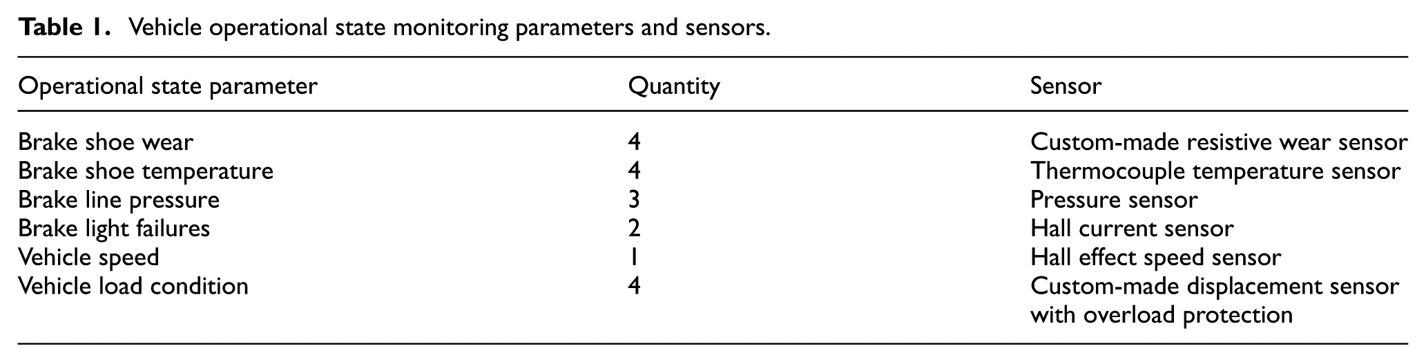
Excessive braking distances in vehicles are a direct cause of rear-end collisions. Factors influencing these braking distances include the initial braking speed of the vehicle, its load condition, braking force, and the road surface adherence conditions. Braking distances serve as a critical indicator of the consistency of braking performance. The temperature and wear level of the brake shoes can reflect the stability of the vehicle’s braking performance.⁹ Additionally, in light of the potential risks posed by brake light malfunctions, the state of the brake lights has also been incorporated into the data collection scheme for braking parameters. After considering the various factors that affect the safety of automotive brakes, a comprehensive method for collecting parameters of the braking system in trucks was proposed. The collected parameters and types of sensors used are detailed in Table 1.

Table 1.

Vehicle operational state monitoring parameters and sensors.

Operational state parameter	Quantity	Sensor
Brake shoe wear	4	Custom-made resistive wear sensor
Brake shoe temperature	4	Thermocouple temperature sensor
Brake line pressure	3	Pressure sensor
Brake light failures	2	Hall current sensor
Vehicle speed	1	Hall effect speed sensor
Vehicle load condition	4	Custom-made displacement sensor with overload protection

A specific model of truck, the FAW Jiefang Sailong, was selected for installation of a brake monitoring system to implement the functions described. Figure 1 illustrates the integration of the test vehicle and the information collection system.

Figure 1.

Vehicle braking state monitoring device: (a) Test vehicle, (b) System integration control box, (c) Vehicle speed sensor, (d) Brake shoe temperature sensor, (e) Brake line pressure sensor, (f) Brake shoe wear sensor, (g) Load condition detection sensor and (h) Brake light failure sensor.

Identification of hazardous states in braking based on single parameters

Abnormal wear in brake shoes

Based on the experimental data of sensor calibration through wear test (Table 2), a relationship was established between the wear amount of the brake shoes and the output voltage of the sensor.

Table 2.

Vehicle operational state monitoring parameters and sensors.

Brake shoe lining wear amount (mm)	Sensor output voltage (V)
0	0.95
1	1.63
2	1.91
3	2.20
4	2.49
5	2.78
6	2.99
7	3.28
8	3.51
9	3.82
10	4.12
11	4.53
12	5.0

The results indicated that a quartic fit was most optimal (Figure 2), leading to the derivation of the following relationship between output voltage and wear amount:

L = 0.0469 U^{4} - 0.751 U^{3} + 4.02 U^{2} - 5.18 U + 1.85

(1)

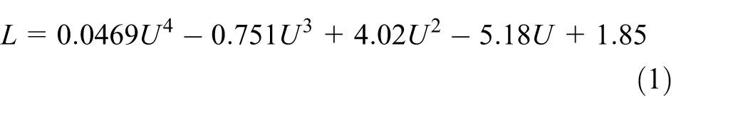
Three mm is the statutory safety threshold for the thickness of the friction plate; vehicles with a thickness below this value will be deemed unqualified during annual inspection.¹⁰ The original thickness of the friction plate of the experimental vehicle is 10 mm; therefore, the safe thickness of the worn friction plate needs to meet: L_w < 7 mm. Substituting into equation (1), the output voltage from the brake shoe wear sensor should be <3.26 volts (V_w < 3.26). This voltage serves as the parameter for identifying abnormal wear in the brake shoes.

Figure 2.

Fitting curve of brake shoe wear extent versus output voltage.

Identification of abnormal temperature states in brake shoes

The temperature of brake shoes in trucks significantly impacts the stability of their braking performance. Figure 3 displays the performance of various material brake shoes in relation to the static friction coefficient and temperature, obtained through experimental studies. Research indicates that when temperatures exceed 250 °C, the friction coefficient of all materials tested shows a significant decline, thereby increasing the risk of brake failure.¹¹

Figure 3.

Friction coefficient curves of different friction materials with temperature variation.

A thermocouple temperature sensor for brake shoes was selected to enable real-time monitoring of temperature changes in vehicle brake shoes. Given the significant impact of sensor placement on monitoring accuracy, this study conducted an ANSYS simulation analysis of temperature changes in the vehicle’s brake lining during braking processes to determine the optimal sensor placement. This simulation analysis facilitates a more precise assessment of the stability of braking performance. Figure 4 shows the temperature field distribution obtained through simulation analysis.

Figure 4.

Temperature field distribution.

The three-dimensional model of the experimental vehicle’s brake shoe was imported into ANSYS, and a mesh was created for simulation analysis. Under conditions of emergency braking with constant braking force, simulation results indicated that the highest temperature of the brake lining friction pad was located in the upper half at a vertical position along the y-axis ranging from y₀ = 90 to 105 mm. In this high-temperature area, a thermocouple temperature sensor was positioned to capture data on the temperature rise of the brake.

According to the Chinese national standard GB5763-2008 “Automobile Brake Linings,” the optimal operating temperature range for brake linings in trucks is between 100 °C and 350 °C. The United States Federal Highway Administration considers the brake drum temperature of trucks during the braking process and sets a critical threshold of 260 °C when planning highway emergency escape lanes.¹² Based on the aforementioned studies, this research sets the hazardous threshold for brake shoe temperature at 260 °C.

Early warning of brake light failures

The status of brake and turn signal lights is monitored using a Hall current sensor. In the event of a brake light failure, the sensor may either fail to detect any voltage or detect an anomalous voltage value. By examining the output voltage state from the Hall current sensor, one can accurately determine the operational status of the vehicle’s lights. Figure 5 illustrates the output voltage signal from the sensor located on the left rear side of the brake test bench, indicating that, during normal operation, the output voltage (U) ranges between 1.9 and 2.0 V.

Figure 5.

Output voltage of the hall current sensor for brake light status.

Identification of multi-parameter brake hazard states

Through a detailed analysis of the braking torque of the test vehicle, we have developed an accurate model that considers multiple critical parameters for trucks under various braking conditions to compute the respective braking distances. These parameters include, but are not limited to, vehicle load, speed, road surface conditions, the coefficient of friction between tires and the ground, and the response time of the braking system. This multi-parameter model for calculating braking distances provides a scientific basis for assessing the safety performance of trucks, thereby guiding vehicle design and improvements. This ensures optimal braking performance in real-world driving conditions, enhancing vehicular safety.

Analysis of braking torque

To ensure consistency between the model and experimental parameters, the braking torque analysis is conducted using an unbalanced camshaft drum brake type, as illustrated in Figure 6. The deformation of the friction lining follows Hooke’s Law.

Figure 6.

Mechanics of the brake system.

The expression for the equivalent braking force over the entire area of the friction lining can be deduced:

F_{μ} = \frac{A \times P \times R \times L_{AS} \times η}{r \times (1 + \cos α \times \frac{m}{\cos β}) \times K \times D_{L} \times \cos θ}

(2)

Where L_AS, K, and D_L are defined as:

D_{L} = \frac{4 \sin (\frac{2}{θ}) \times R_{0}}{θ + \sin θ}

(3)

L_{AS} = \sin α \times (X_{A} - X_{S}) + \cos α \times (Y_{A} + Y_{S})

(4)

K = \frac{L}{R_{0}} \times [\frac{\sin θ \times (μ \times \sin 2 σ + \cos 2 σ) + θ}{4 \times \sin (θ / 2) \times μ \times \cos σ}] - 1

(5)

Calculation model for braking distances

In the analysis of braking processes, particularly under extreme conditions such as pure rolling and locked-wheel skidding, the equation for calculating braking distances is given by:

\begin{matrix} s = \frac{1}{3.6} (τ_{1} + {τ_{2}}^{'} + \frac{{τ_{2}}^{″}}{2}) \cdot v_{0} + \frac{{v_{0}}^{2}}{25.92 \cdot a_{b max}} \\ {\begin{matrix} a_{b max} = \frac{F_{μ} + F_{W} + F_{i} + F_{f}}{m} F_{μ} < F_{ϕ b max} \\ a_{b max} = \frac{F_{ϕ} + F_{W} + F_{i} + F_{f}}{m} F_{μ} \geq F_{ϕ b max} \end{matrix} \\ F_{φ} = φ_{b} G \end{matrix}

(6)

Where {\varphi _b} represents the road adhesion coefficient and G denotes the gravitational force of the vehicle.

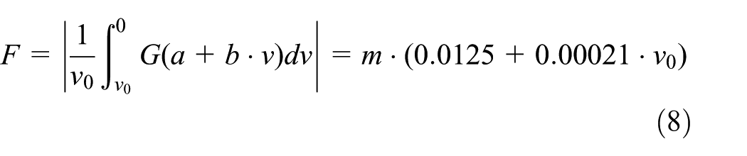
The equations for calculating air resistance, F_W, and rolling resistance, F_f, as specified in equation (6), can be derived in accordance with the national standard “GB12676-2014 Technical requirements and testing methods for commercial vehicle and trailer braking systems.” The test vehicle used is the Jiefang Sailong CA1169PK2L2EA80 truck, with vehicle parameters as listed in Table 1. The coasting tests are conducted on a 10 km flat and dry asphalt concrete road which is seldom used by other vehicles and free of disturbances,¹³ as illustrated in Figure 7. These experiments determine the coefficients of rolling resistance and air resistance of the vehicle. According to Delaigue and Eskandarian,³ the experimental conditions should include a dedicated test track, typically flat, dry, and hard surfaced, measuring 2–3 km in length and at least 8 m in width, with a longitudinal gradient within 0.1%. Wind speed should not exceed 3 m/s, atmospheric temperature should range between 0 °C and 40 °C, and atmospheric pressure should be between 80 and 110 kPa. During the test, the vehicle initially travels at a steady speed slightly above 50 km/h, then the clutch pedal is rapidly depressed, and the vehicle is shifted into neutral to coast until it comes to a stop. Simultaneously, measurements of coasting time and distance are recorded using a fifth wheel device or equivalent speed, travel, and time recording equipment (Table 3).

{\bar{F}}_{W} = | \frac{1}{v_{0}} \int_{v_{0}}^{0} \frac{C_{D} A v^{2}}{21.15} dv | = 0.039 {v_{0}}^{2}

(7)

F = | \frac{1}{v_{0}} \int_{v_{0}}^{0} G (a + b \cdot v) dv | = m \cdot (0.0125 + 0.00021 \cdot v_{0})

(8)

Figure 7.

Difference between test and simulation results for an unladen vehicle (4810 kg).

Table 3.

Full vehicle parameters of the test vehicle.

Vehicle parameter	Parameter value	Vehicle parameter	Parameter value
Vehicle type	N3	Curb weight (kg)	4780
Total vehicle mass (kg)	15,000	Wheelbase (mm)	4910
Mass (kg)	9900	Wheel rolling radius (mm)	465
Tire specification	8.25–20	Cabin height (mm)	2155
Cabin width (mm)	1960	Rearview mirror area (m²)	0.0924

From equations (6) to (8), the equation for calculating the stopping distance on a horizontal road surface for the test vehicle is derived:

s = \frac{1}{3.6} (τ_{1} + {τ_{2}}^{'} + \frac{{τ_{2}}^{″}}{2}) \cdot v_{0} + \frac{{v_{0}}^{2}}{25.92 \cdot a_{b max}}

(9)

{\begin{matrix} a_{b max} = \frac{F_{μ} + 0.039 \cdot {v_{0}}^{2} + m \cdot (0.0125 + 0.00021 \cdot v_{0})}{m} F_{μ} < F_{ϕ} \\ a_{b max} = \frac{F_{ϕ} + 0.039 \cdot {v_{0}}^{2} + m \cdot (0.0125 + 0.00021 \cdot v_{0})}{m} F_{μ} \geq F_{ϕ} \end{matrix}

Analysis of parking distance model experiments

Simulation experiments

In order to simplify the computational and validation process of the braking distance model, we constructed a simulation model for braking distances using the MATLAB/Simulink platform, based on structural parameters of the experimental vehicle. The specific modeling parameters are detailed in Table 4. Through simulation analysis, we identified the impact of load condition, initial braking velocity, and brake force on the stopping distance. We then derived the braking stopping distances under various combinations of state parameters.

Table 4.

Brake system parameters of experimental trucks.

Brake parameter	Parameter value
A1—Front brake chamber area (in²)	30
A2—Rear brake chamber area (in²)	20
R—Slack adjuster radius (mm)	110
r—Cam base radius (mm)	20
R0—Brake drum radius (mm)	210
L—Distance from the center of the brake drum to the brake shoe support pin (mm)	180
X—Horizontal distance from the cam and brake shoe contact point to the support pin (mm)	12
Y—Vertical distance from the cam and brake shoe contact point to the support pin (mm)	330
α—Pressure angle of the leading shoe’s normal force on the camshaft (°)	25
β—Pressure angle of the trailing shoe’s normal force on the cam (°)	20
θ—Lining wrap angle (°)	110
η—Brake system efficiency	0.75
u—Friction coefficient	0.35
m—Actuation ratio	3.5

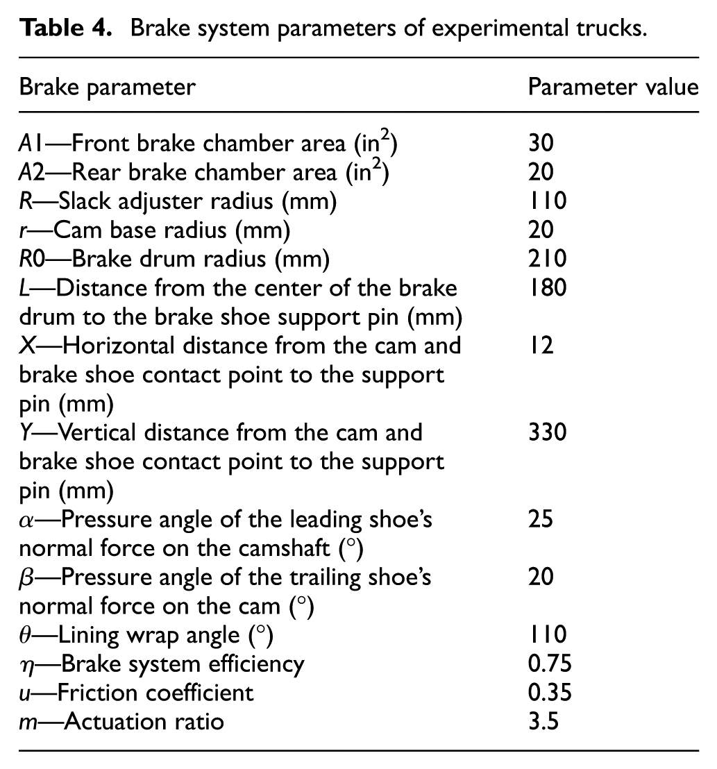
Using the brake system parameters, we input these into the brake force equation (1) to obtain the brake force F_μ:

F_{μ} = 0.0171 \cdot P_{f} + 0.0114 \cdot P_{r}

(10)

P_f represents the front brake line pressure and P_r denotes the rear brake line pressure.

Taking the spot braking pure rolling mode as an example, we established a braking simulation model by combining the stopping distance calculation equations (9) and (10). The simulation employed a braking distance equation derived from F_μ < F. Input variables included initial braking velocity, brake line pressure, and vehicle load, with the output being the stopping distance. The simulation yielded a relationship surface plot between the stopping distance of trucks and variables such as brake line pressure, travel speed, and load mass.

Figure 8 presents a curve illustrating the relationship between velocity, brake pressure, and braking distance under a specified load condition. It is observed that when the truck is at half load (total vehicle mass of 9750 kg), the braking distance is directly proportional to the initial braking speed. Conversely, at a constant speed, the stopping distance is inversely proportional to the brake line pressure.

Figure 8.

Stopping distance surface at half load (9750 kg).

As shown in Figure 9, the surface plot details the relationship between load, braking pressure, and braking distance at an initial braking speed of 70 km/h. It is evident that given a constant initial speed, the stopping distance is directly proportional to the vehicle load. Furthermore, with a constant load mass, the stopping distance inversely correlates with brake line pressure. The simulation results are consistent with the parameters set in the brake tests, and further verification of the accuracy of the braking distance calculation model is conducted through real-vehicle road tests.

Figure 9.

Stopping distance curve at a travel speed of 70 km/h.

On-road vehicle testing

The on-road braking tests for vehicles were conducted on a non-disruptive, straight road surface. The test vehicles, under varying load conditions, utilized brake line valves to control the brake line pressures, conducting fixed-point emergency braking tests at different initial braking speeds. The braking distances were measured using a distance measurement tool. During the braking process, signals such as brake line pressures, traveling speed, and dynamic vehicle load data were collected through a braking status detection device installed on the test vehicle, as depicted in Figure 1. The specific conditions and parameters of the test are listed in Table 5.

Table 5.

Test conditions and parameters.

Item	Parameter value
Test road surface	Long straight concrete road with no slope
Initial braking speed	30, 40, 50, 60
Gross vehicle weight	Unloaded (4810 kg), half load (9750 kg)
Brake circuit valve status	Fully closed, front half open, rear half open, front fully open, rear fully open

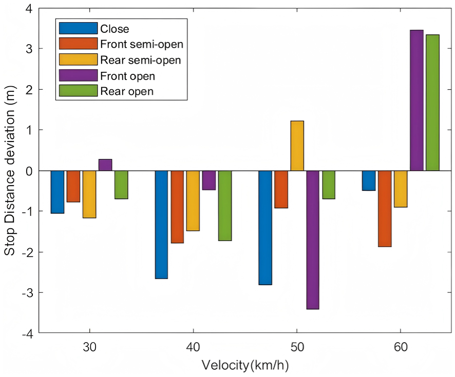
The aforementioned real-vehicle test conditions were also replicated in simulation experiments. Based on a model calculating braking distances, the differences between simulation results and actual braking test outcomes were derived, as shown in Figures 7 and 10.

Figure 10.

Difference between test and simulation results for a half-loaded vehicle (9750 kg).

From the discrepancies noted in Figures 10 and 11, regardless of whether the vehicle was unloaded or half-loaded, the minimum safe driving distance should consider the sum of the emergency braking stopping distance and the safety distance. The safety distance varies under different speeds and road conditions. For instance, on highways, when the speed exceeds 100 km/h, the safety distance should be maintained at over 100 m; for speeds above 60 km/h, the safety distance should be equivalent to the speed (e.g. at 80 km/h, the safety distance should be 80 m). Moreover, according to the Road Traffic Safety Law of the People’s Republic of China, a distance of over 100 m should be maintained from the vehicle ahead in the same lane when visibility is <200 m, and at least 50 m when visibility is under 100 m. Therefore, considering the prediction errors in stopping distances, setting a safety distance of merely 5 m may be overly simplistic. In practice, the safety distance should be adjusted based on specific speeds and road conditions.

Figure 11.

Consideration of the lead vehicle’s braking scenario.

Identification of hazardous states based on following distances

Two scenarios are considered:

First scenario: The lead vehicle executes an emergency brake, followed by the trailing vehicle also initiating emergency braking measures to ensure no collision occurs. Both vehicles come to a stop maintaining a safe distance D as depicted in Figure 11. The braking distance of the lead vehicle is S_f, while that of the trailing vehicle is S_r, with the post-stop distance between the vehicles being DDD and the pre-brake following distance being D₀. The condition for maintaining road safety is thus defined as $s_{f} + D_{0} > s_{r} + D$ .

Second scenario: The lead vehicle comes to a sudden halt due to an obstacle. In this case, it is necessary for the following vehicle to brake emergently and still maintain a safe distance D from the obstacle, as illustrated in Figure 12. Here, the braking distance of the lead vehicle, S_f, is 0. The condition for ensuring driving safety is, where D represents the stopping distance after coming to a halt, typically set at 5 m. Based on the second scenario and taking a conservative estimate, the conservative estimation of the safe following distance D₀ ≥ S_r + 5, where S_r is the braking distance of the trailing vehicle.

During vehicle operation, the vehicle’s braking system monitoring device (Figure 1) detects the vehicle’s status. The braking distance model computes the current braking distance S_stop, predicted as per equation (9). By employing a range sensor to measure the distance D_s between the driving and leading vehicles, a road safety state is determined if the following distance D_s is greater than or equal to S_stop + 5.

Figure 12.

Extreme braking scenario.

Identification of abnormal states in brake line pressures

The experimental trucks selected have a maximum total mass of 15 tons, with two wheels on the front axle and four on the rear axle. According to the motor vehicle classification method in our country, these vehicles fall under category N3. Their required braking distances should satisfy the following equation:

s \leq 0.15 v^{2} + \frac{v^{2}}{103.5}

(11)

Based on the vehicle parameter calibration and calculation results from the braking distance model (equations (9) and (10)), the minimum braking performance requirements for the test vehicle are derived as:

0.2 \cdot v_{0} + \frac{m \cdot {v_{0}}^{2}}{25.92 [0.2315 P + 0.039 \cdot {v_{0}}^{2} + m \cdot (0.0125 + 0.00021 \cdot v_{0})]} \leq 0.15 v_{0} + \frac{{v_{0}}^{2}}{103.5}

(12)

The rules for identifying anomalies in brake line pressures state that changes in the brake line pressures impact the braking distances. Under varying conditions of load and speed, the threshold equation for brake line pressures related to vehicle speed and load is simplified as:

P \geq \frac{17.2486 \cdot m \cdot v_{0}}{v_{0} - 43.9875} - 0.1685 \cdot {v_{0}}^{2} - m \cdot (0.054 + 0.00091 \cdot v_{0})

(13)

Here, m represents the total vehicle mass, determined via load-sensing sensors; $v_{0}$ denotes the vehicle’s driving speed; and P is the pressure value detected by the sensor in the brake lines.

Using the threshold equation, we employed MATLAB software to plot the threshold curve for brake line pressures (Figure 13). Points marked on this surface represent the minimum safe threshold values for brake line pressures, indicating that under all normal conditions, the brake line pressures must remain above this value. This surface acts as a boundary: if the current brake line pressures are below this surface, it is considered a hazardous state; otherwise, it is deemed safe.

Figure 13.

Brake line pressure threshold surface plot.

Conclusion

By analyzing hazardous states and their influencing factors, a vehicle en-route monitoring system was constructed to acquire data on truck load, vehicle speed, and braking system status.

Based on sensor data, hazardous states induced by anomalies such as abnormal wear of brake shoes, excessive temperatures of brake shoes, and brake light failures were identified.

A braking distance calculation model was established based on dynamic analysis during the braking process. To calibrate model parameters, coasting tests for trucks were designed and executed.

The reliability of the vehicle braking distance model was ascertained through simulations using ADAMS software and practical vehicle tests. An analysis of the interplay between following distances, brake line pressures, and braking distances led to the proposal of a new multi-parameter identification method for hazardous states during the braking process.

Footnotes

Handling Editor: Divyam Semwal

ORCID iDs

Bingkui Ji

Yuexi Zhong

Funding

The authors disclosed receipt of the following financial support for the research, authorship, and/or publication of this article: This work was supported by the Talent Introduction Research Initiation Fund Project of Suqian University (Suqian University no. 2023XRC020), Natural Science Foundation of Jilin Province of China (no. 20230101333JC), Suqian University Interdisciplinary Integration Innovation Application Excellent Project under Grant No. School 2024XQT009, 2025 “Suqian Talents” Xiong Ying Plan Talent Introduction Project (no. SQXY202528).

Declaration of conflicting interests

The authors declared no potential conflicts of interest with respect to the research, authorship, and/or publication of this article.

References

Gong

Thoughts on several issues of road traffic safety management in the new era (part 2). Road Traffic Manag 2022; 6(9): 44–47.

Scott

Fay

Hoover

, et al. Brake performance testing and truck runaway analysis. Paper No.2003-01-3396.2003 SAE International Truck and Bus Meeting and Exhibition. Fort Worth: SAE International, 2003.

Delaigue

Eskandarian

A comprehensive vehicle braking model for predictions of stopping distances. J Automob Eng 2004; 218(12): 1409–1417.

Wang

Study on truck speed prediction in long and steep downhill sections. J Highw Transp Res Dev 2017; 34(7): 32.

Shi

Gao

Zhang

, et al. Identification of braking condition for heavy truck on long downhill. Automot Saf Energy 2023; 14(3): 299–309.

Shi

Guo

, et al. Long downhill braking control strategy for heavy-duty truck. J Highw Transp Res Dev 2024; 41(10): 192–202.

Yao

Research on identification and monitoring and early warning for truck statues. Jilin University, 2014.

Qui

Research on optimal control method of combined braking for heavy-duty trucks. Dissertation, Chang’an University, China, 2021.

Automotive theory. 6th ed. China Machine Press, 2018.

10.

China Automotive Maintenance and Repair Association (CAMRA). Survey report on maintenance status of passenger car brake systems (2025 annual). China Automotive Maintenance and Repair Association, 2025.

11.

The experimental research on the temperature rise of drum brake continuance brake in long downhill mountains. Chang’an University, 2008.

12.

Sun

. Study of friction behavior test method for automotive brake. Dissertation, Jilin University, China, 2014.

13.

GB12676-2014. Technical requirements and testing methods for commercial vehicle and trailer braking systems. Standards Press of China, 2014.

Multi-parameter fusion method for hazardous state identification during the braking process of trucks