An integrated computational fluid dynamics and chemical kinetics modeling for predicting oil degradation in maritime diesel engines

Abstract

Graphical abstract

This manuscript presents an integrated approach combining chemical kinetics modeling with computational fluid dynamics (CFD) simulation to investigate oil degradation during the operation of a maritime diesel engine MTU 10V 2000 M72. Using COMSOL Multiphysics 6.2, a detailed 2D simulation was performed to model key engine components, including the main journal bearings, connecting rod journal bearings, piston, and oil pan. Three key parameters were analyzed: heat of combustion, crankshaft rotational speed, and oil flow rate. Results demonstrate that while heat of combustion has a moderate impact on oil lifespan, rotational speed significantly affects degradation due to its influence on temperature and flow conditions. The oil flow rate resulted as the most critical factor, with higher flow rates effectively reducing oil temperature and extending its lifespan by minimizing exposure to elevated temperatures. This study highlights the complex interplay between heat generation, flow dynamics, and chemical degradation, providing insights for improved lubricant performance, predictive maintenance strategies, and enhanced engine reliability.

Introduction

Oil lubricants play a critical role in minimizing wear on mechanical components in constant surface contact. They also protect against corrosion and aid in dissipating heat generated during operation. However, the lifespan of lubricants is constrained by the degradation of their mechanical and chemical properties, which reduces their ability to lubricate, cool, and protect effectively. ¹ This degradation is primarily caused by oxidation, nitration, high operating temperatures, environmental corrosion, shearing, additive depletion, and the accumulation of wear debris. ² To address these issues, chemical additives are incorporated into lubricants to enhance their performance and extend their service life under various operating conditions.

Failure to replace lubricants once their properties are compromised can lead to severe machinery damage and operational failures. Among the critical mechanisms of degradation, oxidation is particularly significant. This process is accelerated by high temperatures, exposure to oxygen, water contamination, and the presence of wear debris.^3–5 Oxidation not only diminishes lubricant effectiveness but also produces harmful byproducts such as sludge and acids, which exacerbate component wear and tear. Therefore, understanding and mitigating these degradation mechanisms is essential for enhancing machinery reliability and reducing maintenance costs.

Currently, lubricant replacement schedules are often based on mileage, with intervals of approximately 5000 miles in the United States and up to 10,000 miles in Europe for automotive engines. ⁶ However, this approach overlooks the operational conditions under which these distances are accumulated. Premature disposal of lubricants still in good condition negatively impacts the environment, while continued use of degraded lubricants leads to engine wear, component failures, and inefficient fuel utilization.

Efforts to maximize lubricant lifespan have included studies on chemical composition monitoring, utilizing techniques such as viscosity variation,^7–9 moisture content analysis, ¹⁰ and spectrometric methods.^11,12 Most of these techniques, however, require periodic sampling of the lubricant, which is time-consuming, costly, and inconvenient.

To address these limitations, in-line sensors have been proposed for real-time monitoring of lubricant conditions. Ghahrizjani et al. ¹³ developed an optical sensor that measures changes in the refractive index of lubricants, relying on the length and diameter of glass fibers in the device. While compact and capable of relating optical properties to lubricant performance, this method requires calibration for specific lubricants and does not directly measure additive depletion or chemical composition. Additionally, Gastops developed an optical technique for monitoring lubricant condition using fluorescence spectroscopy. While this method offers high precision, it requires lubricant sampling and the use of advanced spectroscopy equipment. ¹⁴

Bommareddi ¹⁵ proposed an algorithm predicting oil condition based on operational parameters such as engine temperature, speed, load, and runtime. Similarly, Lukášik^16,17 implemented “live” monitoring for a Mitsubishi Lancer engine, using a Raspberry Pi 4 to process sensor data such as motor temperature, atmospheric humidity, and distance traveled. Tribodiagnostic analysis was used to sample oil and estimate its Total Base Number (TBN), a measure of its neutralizing capacity. Although these methods account for operational conditions, they rely on regression models calibrated for specific engines or lubricants. These models are unreliable for predicting the state of the lubricant, when the engine, the speed, or the specific lubricant differ from the ones used during the experimental tests, ¹⁸ and the range of application to get accurate predictions are only the ranges on which they have been calibrated. Moreover, they fail to directly link lubricant chemical composition to its remaining productive life and are unable to provide component-specific analyses critical for optimization.

Computational Fluid Dynamics (CFD) has been increasingly applied to simulate interactions between lubricants and mechanical components, such as gearboxes, bearings, and pumps. CFD allows the evaluation of different lubricants, engine geometries, and operational conditions, overcoming the limitations of empirical and analytical models. Unlike traditional approaches, which often rely on simplified assumptions and averaged parameters, CFD enables a more detailed representation of transient phenomena, such as local pressure variations, turbulent flow effects, and temperature gradients within lubrication systems. These factors play a crucial role in predicting lubricant behavior, including viscosity changes, shear stresses, and the onset of thermal degradation.

One of the key challenges in predicting lubricant degradation is the spatial variation of temperature and flow conditions throughout the lubrication circuit. The lubricant is subjected to continuous heating and cooling as it circulates through different engine components, such as bearings, pistons, and oil galleries, leading to non-uniform temperature distributions. As a result, estimating degradation rates based solely on average temperatures or outlet temperatures can be misleading, as these values fail to capture localized thermal stresses and oxidation hotspots. CFD addresses this challenge by resolving temperature and velocity profiles at high spatial resolution, providing a more accurate assessment of degradation mechanisms.

Maccioni and Concli ¹⁹ extensively reviewed the state of CFD in lubrication analysis, discussing the advantages and limitations of various methods, including finite difference (FDM), finite element (FEM), and finite volume (FVM) approaches. ²⁰ Among these, FVM is widely used in commercial and open-source solvers due to its ability to conserve mass, momentum, and energy across complex geometries. FEM, on the other hand, provides higher flexibility in modeling solid-fluid interactions, making it suitable for elastohydrodynamic lubrication (EHL) studies.

Mesh strategies, such as static or sliding meshes, local or global remeshing, and adaptive meshing techniques, have been implemented to improve solution accuracy and computational efficiency. For instance, sliding mesh methods allow the simulation of moving components, such as journal bearings, where dynamic film thickness and pressure fluctuations influence lubrication performance. Additionally, local mesh refinement enhances the resolution of critical regions, such as contact interfaces and shear layers, where thermal and mechanical stresses are highly localized.

Advancements in software platforms such as COMSOL Multiphysics, OpenFOAM, and ANSYS have further expanded the capabilities of CFD in lubrication modeling.^21–24 These tools facilitate multi-physics coupling, integrating fluid flow, heat transfer, and chemical reactions to capture the complex interactions governing lubricant degradation. By incorporating detailed thermal and flow field analysis, CFD enables a more precise evaluation of oil oxidation rates, additive depletion, and contaminant transport under varying operating conditions. This approach allows engineers to design lubrication systems that minimize thermal stress, optimize oil circulation, and enhance overall engine efficiency and longevity.

Despite these advancements, a gap remains in coupling CFD with chemical kinetics to accurately predict lubricant degradation and additive depletion. This manuscript proposes a CFD-based framework that models key engine components involved in lubricant degradation, focusing on flow and thermal interactions affecting lubricant reactivity. A simplified 2D representation of engine elements was developed to reduce computational demands.

The proposed CFD and chemical kinetics simulation system can predict lubricant condition at any stage without requiring laboratory sampling, using engine parameters such as temperature, flow rate, and rotational speed.^{8,9,13,16,17,19,22–24} These parameters can be recorded by sensors and analyzed periodically or in real-time using onboard computers. This approach enables continuous monitoring of lubricant state and productive life, providing actionable insights to reduce lubricant waste, enhance performance, and optimize maintenance schedules. Figure 1 illustrates the proposed framework for predicting lubricant condition and remaining productive life.

Figure 1.

Diagram of the proposed solutions for predicting lubricant condition and remaining productive life. The system enables periodic or live monitoring of lubricant state.

Computational modeling

Fluid dynamics model

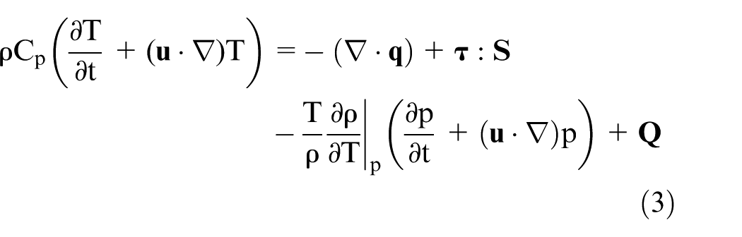
The general single-phase flow theory was implemented for the fluid dynamics simulation. This approach is based on the Navier-Stokes equations. Equation (1) describes the continuity equation that represents the conservation of mass. Equation (2) describes a vector equation that represents the conservation of momentum. Equation (3) describes the conservation of energy in terms of temperature. Equation (4) describes the strain-rate tensor, and equation (5) describes a linear relationship between stress and strain for a Newtonian fluid.^25,26

$$\frac{\partial \mathrm{\rho }}{\partial \mathrm{t}}+\nabla ·\left(\mathrm{\rho }\mathbf{u}\right)=0$$

(1)

$$\mathrm{\rho }\frac{\partial \mathbf{u}}{\partial \mathrm{t}}+\mathrm{\rho }(\mathbf{u}·\nabla )\mathbf{u}=\nabla ·[-\mathrm{p}\mathbf{I}+\mathbf{\tau }]+\mathbf{F}$$

(2)

$$\begin{array}{c}\multicolumn{1}{c}{\mathrm{\rho }{\mathrm{C}}_{\mathrm{p}}(\frac{\partial \mathrm{T}}{\partial \mathrm{t}}+(\mathbf{u}·\nabla )\mathrm{T})=-(\nabla ·\mathbf{q})+\mathbf{\tau }:\mathbf{S}}\\ \multicolumn{1}{c}{-{\frac{\mathrm{T}}{\mathrm{\rho }}\frac{\partial \mathrm{\rho }}{\partial \mathrm{T}}|}_{\mathrm{p}}(\frac{\partial \mathrm{p}}{\partial \mathrm{t}}+(\mathbf{u}·\nabla )\mathrm{p})+\mathbf{Q}}\end{array}$$

(3)

$$\mathbf{S}=\frac{1}{2}(\nabla \mathbf{u}+{(\nabla \mathbf{u})}^{\mathrm{T}})$$

(4)

$$\mathbf{\tau }=2\mathrm{\mu }\mathbf{S}-\frac{2}{3}\mathrm{\mu }(\nabla ·\mathbf{u})\mathbf{I}$$

(5)

where $\mathrm{\rho }$ is the density of the fluid (kg/m³), u is the velocity vector (m/s), p is the pressure (Pa), $\mathbf{\tau }$ is the viscous stress tensor (Pa), F is the volume force vector (N/m³), ${\mathrm{C}}_{\mathrm{p}}$ is the specific heat capacity at constant pressure (J/(kg·K)), T is the absolute temperature (K), q is the heat flux vector (W/m²), Q contains the heat source (W/m³), I is the identity tensor, S is the strain-rate tensor, and $\mathrm{\mu }$ is the dynamic viscosity (Pa·s).

Heat transfer model

The heat transfer in solids and fluids theory, represented by equation (6), was implemented to compute the temperature field.^26,27

$$\mathrm{\rho }{\mathrm{C}}_{\mathrm{p}}(\frac{\partial \mathrm{T}}{\partial \mathrm{t}}+\mathbf{u}·\nabla \mathrm{T})+\nabla ·\mathbf{q}={\mathbf{Q}}_{\mathrm{ted}}+\mathbf{Q}$$

(6)

where $\mathrm{\rho }$ is the density (kg/m³), ${\mathrm{C}}_{\mathrm{p}}$ is the specific heat capacity at constant stress (J/( $\mathrm{kg}·\mathrm{K}$ )), T is the absolute temperature (K), u is the velocity vector (m/s), Q includes additional heat sources (W/m³), $\mathbf{q}$ is the heat flux (W/m²), and ${\mathbf{Q}}_{\mathrm{ted}}$ accounts for thermoelastic damping, capturing thermoelastic effects in solids as defined in equation (7).

$${\mathbf{Q}}_{\mathrm{ted}}=-\mathrm{\alpha }\mathrm{T}:\frac{\mathrm{d}\mathbf{S}}{\mathrm{dt}}$$

(7)

Where $\mathrm{\alpha }$ is the coefficient of thermal expansion (1/K), and S is the second Piola-Kirchhoff stress tensor (Pa).

Transport of diluted species

The transport of diluted species module was used to solve for the chemical kinetics reaction. This interface provides a modeling environment for studying the evolution of chemical species transported by diffusion. ²⁸ Equation (8) shows the mass conservation for one or more chemical species i,

$$\frac{\partial {\mathrm{c}}_{\mathrm{i}}}{\partial \mathrm{t}}+\nabla ·{\mathbf{J}}_{\mathrm{i}}+\mathbf{u}·\nabla {\mathrm{c}}_{\mathrm{i}}={\mathrm{R}}_{\mathrm{i}}$$

(8)

where ${\mathrm{c}}_{\mathrm{i}}$ is the concentration of the species (mol/m³), ${\mathrm{R}}_{\mathrm{i}}$ is a reaction rate expression for the species (mol/m³s), u is the mass-averaged velocity vector (m/s), and ${\mathbf{J}}_{\mathrm{i}}$ is the mass flux diffusive flux vector (mol/m²s) as described in equation (9), where ${\mathrm{D}}_{\mathrm{i}}$ denotes the diffusion coefficient (m²/s).

$${\mathbf{J}}_{\mathrm{i}}=-{\mathrm{D}}_{\mathrm{i}}\nabla {\mathrm{c}}_{\mathrm{i}}$$

(9)

Chemical kinetics degradation model of lubricants

Omrani et al. ²⁹ proposed a lubricant composition model based on an additive phenyl-α-naphthylamine PANH, considering the radical product as ${\mathrm{PAN}}^{•}$ , and the dimer as PAN₂. The primary radical oxidation products react with PANH to produce its dimer, PAN₂. Once PANH and PAN₂ have been removed, oxidation occurs in the remaining compounds which have higher oxidation stability. One of these compounds was an unidentified antioxidant which was designed as AO. Once the antioxidants AO, PANH, and PAN₂ have been depleted, the lubricant will be then oxidized. A simplified model was proposed as follows:

$$\begin{array}{c}\mathrm{RH}+{\mathrm{O}}_2\to {\mathrm{R}}^{•}+{\mathrm{HO}}_2^{•}\hfill \\ {\mathrm{R}}^{•}+{\mathrm{O}}_2\to {\mathrm{ROO}}^{•}\hfill \end{array}$$

$$\begin{array}{c}{\mathrm{ROO}}^{•}+\mathrm{RH}\to {\mathrm{R}}^{•}+\mathrm{ROOH}\hfill \\ {\mathrm{HO}}_2^{•}+\mathrm{RH}\to {\mathrm{H}}_2{\mathrm{O}}_2+{\mathrm{R}}^{•}\hfill \\ \mathrm{ROOH}\to {\mathrm{OH}}^{•}+{\mathrm{RO}}^{•}({\mathrm{RR}}^{\prime }{\mathrm{HCO}}^{•},{\mathrm{RR}}^{\text{'}}{\mathrm{R}}^{″}{\mathrm{CO}}^{•})\hfill \\ {\mathrm{RO}}^{•}+\mathrm{RH}\to \mathrm{ROH}+{\mathrm{R}}^{•}\hfill \\ {\mathrm{HO}}^{•}+\mathrm{RH}\to {\mathrm{H}}_2\mathrm{O}+{\mathrm{R}}^{•}\hfill \end{array}$$

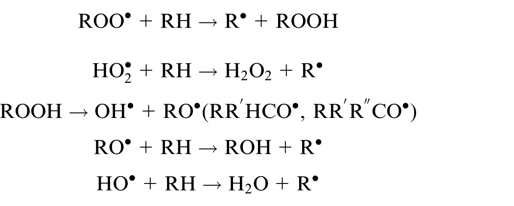
Where the oxyradical RO can be primary, secondary, or tertiary depending on the position of the initial CH bond cleavage. The secondary and tertiary oxyradicals can be further decompose into aldehydes and ketones.

$$\begin{array}{c}{\mathrm{RR}}^{\prime }{\mathrm{HCO}}^{•}\to {\mathrm{R}}^{\prime }\mathrm{CHO}+{\mathrm{R}}^{•}\hfill \\ {\mathrm{RR}}^{\prime }{R}^{″}{\mathrm{CO}}^{•}\to {\mathrm{R}}^{\prime }{R}^{″}\mathrm{CO}+{\mathrm{R}}^{•}\hfill \end{array}$$

If antioxidants such PANH are present, the radicals are scavenged and converted into stable compounds.

$$\mathrm{PANH}+{\mathrm{R}}^{•}{\to }^{{\mathrm{k}}_1}{\mathrm{PAN}}^{•}+\mathrm{RH}\mathrm{where}\mathrm{R}=\mathrm{R},\mathrm{RO},\mathrm{RC}{\mathrm{O}}_2,$$

etc.

$$\begin{array}{c}2{\mathrm{PAN}}^{•}{\to }^{{\mathrm{k}}_2}{\mathrm{PAN}}_2\hfill \\ {\mathrm{PAN}}_2+{\mathrm{R}}^{•}{\to }^{{\mathrm{k}}_3}\left(\mathrm{Product}\right)+\mathrm{RH}\hfill \\ \mathrm{AO}+{\mathrm{R}}^{•}{\to }^{{\mathrm{k}}_4}\left(\mathrm{Product}\right)+\mathrm{RH}\hfill \end{array}$$

Reaction rate equations are then defined as follows:

$$\frac{\mathrm{d}[\mathrm{PANH}]}{\mathrm{dt}}=-{\mathrm{k}}_1[\mathrm{PANH}][{\mathrm{R}}^{•}]$$

(10)

$$\frac{\mathrm{d}[{\mathrm{PAN}}^{•}]}{\mathrm{dt}}={\mathrm{k}}_1\left[\mathrm{PANH}\right]\left[{\mathrm{R}}^{•}\right]-{\mathrm{k}}_2[{\mathrm{PAN}}^{•}{]}^2$$

(11)

$$\frac{\mathrm{d}[{\mathrm{PAN}}_2]}{\mathrm{dt}}={\mathrm{k}}_2[{\mathrm{PAN}}^{•}{]}^2-{\mathrm{k}}_3[{\mathrm{PAN}}_2]\left[{\mathrm{R}}^{•}\right]$$

(12)

$$\frac{\mathrm{d}[\mathrm{AO}]}{\mathrm{dt}}=-{\mathrm{k}}_4[\mathrm{AO}]\left[{\mathrm{R}}^{•}\right]$$

(13)

The following assumptions were made:

1. The reaction rate of AO is slower than that of PANH, where ${\mathrm{k}}_4<{\mathrm{k}}_1$ .

2. The concentration of PAN-radicals is constant, while PANH is at large excess over the organic radicals $\left[{\mathrm{R}}^{•}\right]$ , such that ${\mathrm{k}}_1\left[\mathrm{PANH}\right]\left[{\mathrm{R}}^{•}\right]={\mathrm{k}}_2[{\mathrm{PAN}}^{•}{]}^2$ .

3. The concentration of organic radicals is constant while PANH is at large excess over these radicals, such that ${\mathrm{k}}_1^{\prime }={\mathrm{k}}_1\left[{\mathrm{R}}^{•}\right]$ , ${\mathrm{k}}_2^{\prime }={\mathrm{k}}_2\left[{\mathrm{R}}^{•}\right]$ , ${\mathrm{k}}_3^{\prime }={\mathrm{k}}_3\left[{\mathrm{R}}^{•}\right]$ .

Equations (10), (12), and (13) can be re-written as follows:

$$\frac{\mathrm{d}[\mathrm{PANH}]}{\mathrm{dt}}=-{\mathrm{k}}_1^{\prime }[\mathrm{PANH}{]}_0$$

(14)

$$\frac{\mathrm{d}[{\mathrm{PAN}}_2]}{\mathrm{dt}}={\mathrm{k}}_1^{\prime }[\mathrm{PANH}{]}_0-{\mathrm{k}}_3^{\prime }[{\mathrm{PAN}}_2{]}_0$$

(15)

$$\frac{\mathrm{d}[\mathrm{AO}]}{\mathrm{dt}}=-{\mathrm{k}}_4^{\prime }[\mathrm{AO}{]}_0$$

(16)

$${\mathrm{k}}_{\mathrm{i}}^{\prime }={\mathrm{A}}_{\mathrm{i}}{\mathrm{e}}^{\frac{-{\mathrm{E}}_{\mathrm{ai}}}{\mathrm{RT}}}$$

(17)

where ${\mathrm{E}}_{\mathrm{ai}}$ is the activation energy (kJ/mol) and R is the gas constant (8.314 J/K mol). Assuming that PAN-radicals and $\left[{\mathrm{R}}^{•}\right]$ organic radicals remain constant is consistent with a well-aerated oxygen rich system. ²⁹

Two-dimensional representation of the engine elements

A maritime diesel engine from MTU, specifically the 10 V 2000 MT2 motor, was used for this computational analysis. Figure 2 illustrates the schematic of the lubrication system. The oil is stored in the oil tank and distributed via the engine oil pump through a strainer. It then passes through the engine oil heat exchanger, the oil filters, and the main oil gallery, before being injected into the camshaft bearings, the head pistons, and the crankshaft bearings. The oil eventually returns to the oil tank, except for the oil passing through the crankshaft bearings, which flows to the connecting rod bearings before returning to the oil tank.

Figure 2.

Schematic of the lubrication system for the maritime engine.

Only the main components involved in the chemical reactions of the lubricant were analyzed in this research. These components experience high-temperature variations and constant flow. To ensure flow continuity between the elements, an average out-of-plane thickness was assumed. The height of the oil tank (H_t) was adjusted to match the same volume under the average thickness between the journal bearings. Figure 3 highlights the main engine elements influencing the chemical reaction, such as the piston, where heat is generated in the combustion chamber. The heat transfers to the connecting rod journal bearings and the main journal bearings through the crankshaft.

Figure 3.

Schematic of the main elements (piston, main journal bearing, and connecting rod journal bearing) and the cross-section considered for the 2D analysis.

COMSOL Multiphysics includes an integrated mesh generator that automatically optimizes element size using a physics-controlled mesh. This approach refines the mesh in regions where complex interactions are expected, such as fluid–solid interaction, heat transfer, or chemical reaction zones. Additional control is available by selecting a global mesh size setting (e.g. Normal, Fine, Coarse). For this model, the Fine option was selected. The resulting number of elements and the element size distribution are shown in the mesh visualizations in Figures 4 to 7. A time-dependent solver was used for all simulations, implementing the default backward differentiation formula for time stepping. An initial time step of 1E-6 s was specified to ensure stable initial convergence of the system.

Figure 4.

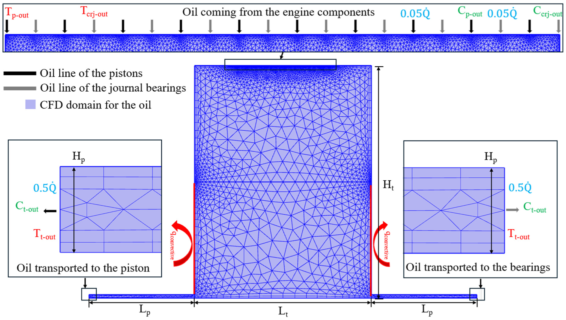
Simplified 2D geometry of the oil tank with the mesh. The flow (in blue), thermal (in red), and chemical concentration (in green) boundary conditions are defined.

Figure 5.

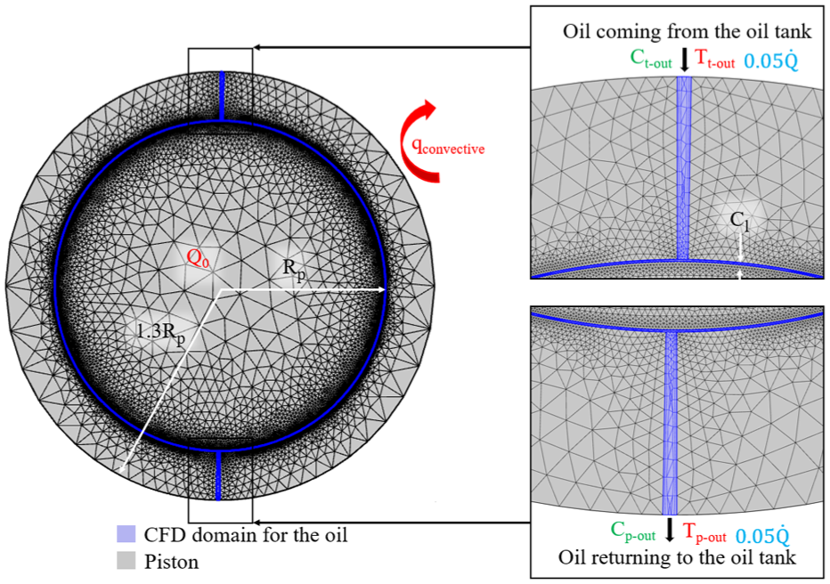
Simplified 2D geometry of the piston with the mesh. The flow (in blue), thermal (in red), and chemical concentration (in green) boundary conditions are defined.

Figure 6.

Simplified 2D geometry of the main journal bearings with the mesh. The flow (in blue), thermal (in red), and chemical concentration (in green) boundary conditions are defined.

Figure 7.

Simplified 2D geometry of the connecting rod journal bearings with the mesh. The flow (in blue), thermal (in red), and chemical concentration (in green) boundary conditions are defined.

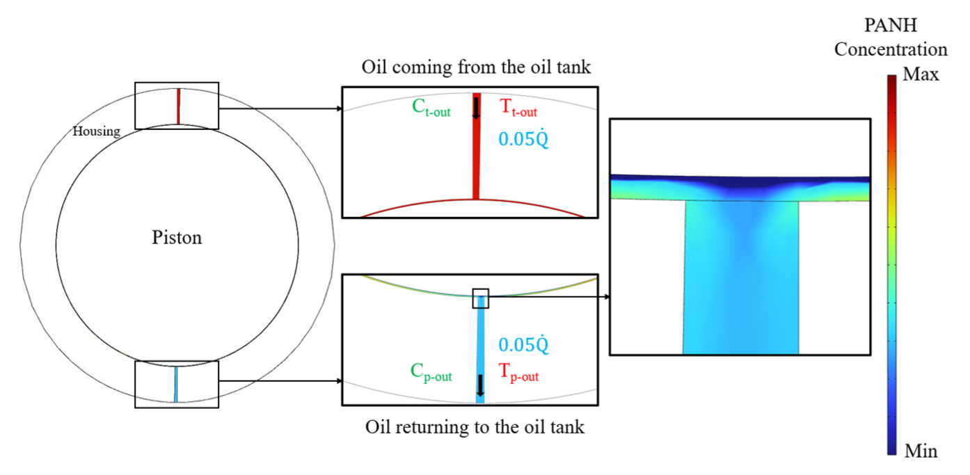
Figure 4 shows the representation of the oil tank. The mesh comprises 4324 triangle elements and 596 quadrilateral elements. The flow boundary conditions are defined along the upper surface, alternating and distributed from the pistons and journal bearings. The injected oil mixes with the stored oil to reach an equilibrium in temperature and chemical concentration. The oil is subsequently extracted and redirected to the pistons and journal bearings. The flow is divided equally, with half directed to the 10 pistons and the other half to the 6 main journal bearings. Thermal boundary conditions assign the inlet flow temperatures to match the oil temperatures exiting the pistons and journal bearings. A similar continuity boundary condition is applied to chemical concentration. Chemical interaction with the environment is considered though the assumption of a constant radical concentration, which is effectively due to excess oxygen. Reaction with any other environmental gases or contaminants is neglected as oxidation is expected to be the dominant mechanism of degradation. Natural convection is assumed for the lower half of the oil tank surfaces to facilitate cooling from the engine elements. This assumption is made based on the portion of the tank that is exposed to the environment. Figure 4 shows the geometry, mesh, and flow-thermal-chemical boundary conditions for the oil tank.

The piston consists of 49,659 triangle elements and 6982 quadrilateral elements, as shown in Figure 5. Each piston receives 0.05 of the total flow rate ( $\stackrel{·}{\mathrm{Q}}$ ). The oil is injected at the same temperature and chemical concentration as the oil extracted from the oil tank. Heat generated during combustion (Q₀) is applied to the piston surface, and convection is assumed on the external surface. The oil exits the piston at a higher temperature and with altered chemical composition.

The main journal bearing comprises 46,918 triangle elements and 7420 quadrilateral elements, as shown in Figure 6. Each main journal bearing receives 0.083 of the total flow rate ( $\stackrel{·}{\mathrm{Q}}$ ). The oil is injected at the same temperature and chemical concentration as the oil extracted from the oil tank. A fraction (0.2) of the heat generated during combustion (Q₀) is transmitted from the piston to the main journal bearings, and convection is applied to the external surface. The oil exits at a higher temperature and with a different chemical composition.

The connecting rod journal bearing consists of 38,652 triangle elements and 6106 quadrilateral elements, as shown in Figure 7. Each connecting rod journal bearing receives 0.05 of the total flow rate ( $\stackrel{·}{\mathrm{Q}}$ ). The oil is injected at the same temperature and chemical concentration as the oil extracted from the main journal bearing. A fraction (0.2) of the heat generated during combustion (Q₀) is transmitted from the piston to the connecting rod journal bearings, and convection is applied to the external surface. The oil exits at a higher temperature and with a different chemical composition.

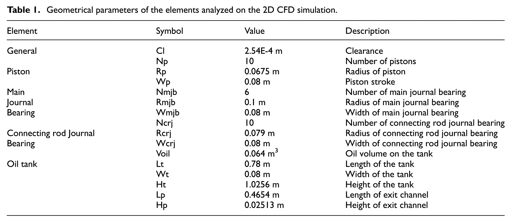
The geometric dimensions were obtained from the literature^30,31 and are detailed in Table 1. These dimensions can be adjusted, and the model will update accordingly to ensure an accurate representation of any specific engine system. The variables described into the boundary conditions for Figures 4 to 7 and the relationships between the elements are described in Table 2.

Table 1.

Geometrical parameters of the elements analyzed on the 2D CFD simulation.

Element	Symbol	Value	Description
General	Cl	2.54E-4 m	Clearance
	Np	10	Number of pistons
Piston	Rp	0.0675 m	Radius of piston
	Wp	0.08 m	Piston stroke
Main	Nmjb	6	Number of main journal bearing
Journal	Rmjb	0.1 m	Radius of main journal bearing
Bearing	Wmjb	0.08 m	Width of main journal bearing
	Ncrj	10	Number of connecting rod journal bearing
Connecting rod Journal	Rcrj	0.079 m	Radius of connecting rod journal bearing
Bearing	Wcrj	0.08 m	Width of connecting rod journal bearing
	Voil	0.064 m3	Oil volume on the tank
Oil tank	Lt	0.78 m	Length of the tank
	Wt	0.08 m	Width of the tank
	Ht	1.0256 m	Height of the tank
	Lp	0.4654 m	Length of exit channel
	Hp	0.02513 m	Height of exit channel

Table 2.

Variables for the elements on the model.

Variable	Description	Relationship with other elements
$\stackrel{·}{\mathrm{Q}}$	Oil flow rate	Half of the flow rate from the tank goes to the pistons, while the other half goes to the journal bearings.
qconvective	Convective heat flow	Convective heat transfer is assumed on the external surfaces of the piston and journal bearings, as well as on the lower half surfaces of the oil tank. A heat transfer coefficient (h) of 10 W/m2K is applied.
Tt-out	Temperature of the oil at the exit of the oil tank	The temperature of the oil exiting the oil tank is assigned as the inlet temperature for both the main journal bearing and the piston.
Ct-out	Oil chemical concentrations at the exit of the oil tank	The chemical concentration of the oil exiting the oil tank is assigned as the inlet chemical concentration for both the main journal bearing and the piston.
Q0	Heat at the piston form combustion	A 10% portion of the heat generated from combustion is assumed to be transferred to the crankshaft and subsequently to the journal bearings.
Tp-out	Temperature of the oil at the exit of the piston	The temperature at which the oil exits the piston is assigned as the temperature at which the oil is returned to the oil tank.
Cp-out	Oil chemical concentrations at the exit of the piston	The chemical concentrations at which the oil exits the piston are assigned as the chemical concentrations at which the oil is returned to the oil tank.
Tmjb-out	Temperature of the oil at the exit of the main journal bearing	The temperature at which the oil exits the main journal bearing is assigned as the temperature at which the oil is introduced into the connecting rod journal bearing.
Cmjb-out	Oil chemical concentrations at the exit of the main journal bearing	The chemical concentrations at which the oil exits the main journal bearing are assigned as the chemical concentrations at which the oil is introduced into the connecting rod journal bearing.
ω	Rotational speed of the crankshaft	The same rotational speed is assigned to both the main journal bearing and the connecting rod journal bearing.
Tcrj-out	Temperature of the oil at the exit of the connecting rod journal bearing	The temperature at which the oil exits the connecting rod journal bearing is assigned as the temperature at which the oil is returned to the oil tank.
Ccrj-out	Oil chemical concentrations at the exit of the connecting rod journal bearing	The chemical concentrations at which the oil exits the connecting rod journal bearing are assigned as the chemical concentrations at which the oil is returned to the oil tank.

Materials and methodology

Standard materials from the COMSOL library were used for the thermal and mechanical properties, such as “Structural Steel” for the engine components and “Engine Oil” for the lubricant. These properties are summarized in Tables 3 and 4.

Table 3.

Thermo-mechanical properties of engine components from COMSOL database.

Property	Structural steel
Heat capacity at constant pressure (J/(kg K))	475
Thermal conductivity (W/(m K))	44.5
Density (kg/m3)	7850
Coefficient of thermal expansion (1/K)	12.3E-6
Young modulus (Pa)	Function of temperature T (K)
	2.1958E11–6.68E7*T
Poisson’s ratio	Function of temperature T (K)
	0.2912+3E-5*T

Table 4.

Thermo-mechanical properties of engine components from COMSOL database.

Property	Engine oil. Properties as function of Temperature T (K).
Heat capacity at constant pressure (J/(kg.K))	761.405625+3.47685606*T+0.00115530303*T2
Thermal conductivity (W/(m.K))	0.192223542-2.0637987E-4*T+1.54220779E-7*T2
Density (Kg/m3)	1068.70404-0.6393421*T+7.34307359E-5* T2
Dynamic viscosity (Pa.s) [32]	273 K<T< 353 K
	42669.28688622
	−741.1718801282*T+5.360521287088*T2
	−0.02066027676164*T3+4.47491538052E-5*T4
	−5.164053479202E-8*T5+2.48033770504E-11*T6
	353 K<T< 433 K
	4.94593941-0.0351869631*T+8.37935977E-5*T2
	−6.67125E-8* T3
	433 K<T
	0.0045

Omrani et al. ²⁹ performed the chemical kinetics characterization of a commercial jet turbine oil (NYCO, jet turbine oil, MIL-PRF-23699 F Class STD). Table 5 shows the parameters for the equations (14)–(17).

Table 5.

Chemical kinetics parameters for NYCO MIL-PRF-23699 F Class STD oil.

Parameter	Value
[PANH]0 (mol/m3)	2275
[PAN2]0 (mol/m3)	0
[AO]0 (mol/m3)	1000
R (J/K mol)	8.314
A1 (1/s)	1.6821E7
Ea1 (J/mol)	93,000
A3 (1/s)	5.8317E8
Ea3 (J/mol)	1.14E5
A4 (1/s)	4.0409E8
Ea4 (J/mol)	1.16E5

Computational analysis

The purpose of this work is to identify the influence of operational parameters on the life cycle of lubricant additives, with special interest in regions of the system where the chemical reaction is more likely to occur. The operational parameters involved in this analysis are as follows: First, the heat of combustion (Q), which is directly linked to the temperature profile. Values ranging from 4E5 to 8E5 W/m² give a temperature range of 1000°C–1800°C at the piston, where combustion occurs, as reported by Manecer et al. ³³ The second parameter is the rotational speed of the journal, which is linked to the flow speed of the oil in contact with the journal. Reported values range between 2000 and 4000 rpm, as reported by Liu. ³⁴ The third parameter is the flow rate of the oil system, which is also linked to the flow speed into the system. Liu ³⁴ reported an oil flow rate of around 6.20E-4 m³/s, and values between 6.0E-4 and 6.5E-4 m³/s are chosen for this analysis.

Table 6 shows the proposed simulations to determine the time at which the lubricant additives are reduced to a critical point, where oxidation of the lubricant is expected to begin.

Table 6.

Computational analysis methodology.

Parameter	Simulation 1. Variation of heat of combustion.	Simulation 2. Variation of rotational speed of the journal.	Simulation 3. Variation of the lubricant flow rate.
Heat of combustion ${\mathrm{Q}}_0$ (W/m2)	4.00E+5, 5.00E+5, 6.00E+5, 7.00E+5, 8.00E+5	6.00E+5	6.00E+5
Rotational speed of the journal ω (rpm)	3000	2000, 2500, 3000, 3500, 4000	3000
Lubricant flow rate $\stackrel{·}{\mathrm{Q}}$ (m3/s)	6.25E-4	6.25E-4	6.00E-4, 6.25E-4, 6.5E-4

Results and discussions

Baseline simulation

We start with a baseline simulation with intermediate process values as a point of comparison for when we vary the parameters later. The baseline simulation uses a heat of combustion of 6.00E+5 W/m², a journal rotational speed of 3000 rpm, and an oil flow rate of 6.25E-4 m³/s. Figure 8 illustrates the temperature profile of the piston at thermal equilibrium. The profile is shown along a cutting line that starts at the oil injection point, follows the piston diameter, and ends at the oil exit. The cooling effect of the oil is evident, with lower temperatures near the injection area and higher temperatures toward the exit. The oil temperature rises from 57°C at the injection point to 195°C at the exit. The maximum temperature at the piston center reaches 1000°C, which aligns with the operational temperature range reported by Manecer et al. ³³

Figure 8.

Temperature profile of the piston: Lower temperatures are observed at the oil inlet to the system. The oil enters at 57°C and exits back to the oil tank at 159°C. Refer to Figure 5 for detailed geometry.

Figures 9 and 10 present the flow speed profiles for the piston and the connecting rod journal bearing. In Figure 9, the flow profile reveals higher speeds at the center of the clearance space, which aligns with the stationary surfaces of the piston and the housing that move linearly in an out-of-plane direction. Conversely, Figure 10 depicts a distinct flow pattern, with higher speeds near the surface of the connecting rod and lower speeds at the housing. This behavior is expected, as the connecting rod is assumed to rotate while the housing remains stationary.

Figure 9.

Piston flow speed profile: As the piston moves linearly out of plane without rotation, the maximum flow speed is observed at the center of the clearance space.

Figure 10.

Flow speed profile for the connecting rod journal bearing: A similar profile is observed in the main journal bearing. Here, the crankshaft’s rotational motion results in maximum flow speed at the surface in contact with the crankshaft and minimum flow speed at the fixed bearing housing.

Figures 11 and 12 illustrate the chemical concentration reactions during oil flow through the piston and journal bearings. In Figure 11, the PANH concentration is highest near the injection point in the piston and gradually decreases as the oil flows through the clearance space, absorbing heat from combustion. A lower concentration is observed at the piston surface, where higher temperatures accelerate degradation. Similar trends are observed for the other chemical components, PAN₂ and AO.

Figure 11.

PANH concentration in the piston: The PANH concentration is highest near the injection channel and decreases toward the exit channel due to heat absorption and component degradation. Similar concentration profiles are also observed for the other chemical components, PAN₂ and AO.

Figure 12.

PANH concentration in the main journal bearing: Similar profiles are observed in the connecting rod journal bearing. The PANH concentration is highest near the injection channel and decreases toward the exit channel due to heat absorption and component degradation. Comparable profiles are also observed for the other chemical components, PAN₂ and AO.

Figure 12 illustrates the behavior of the chemical concentration reaction within the journal bearings. Similar to the piston, the oil exhibits a higher chemical concentration near the injection point and a lower concentration at the exit. However, in this case, the minimum concentration does not occur at the surface with the highest temperature, which is the rotating surface. This is because, despite the elevated temperature, the higher flow speed at the rotating surface reduces the exposure time of the oil to heat-induced degradation. Conversely, near the fixed surface, the lower flow speed prolongs the exposure of the oil to high temperatures, resulting in the degradation profile observed in this figure.

Figure 13 presents the simulation results of the oil tank. The oil enters the tank from the pistons and journal bearings with a higher temperature and a lower PANH chemical concentration. Similar trends are observed for the other chemical components, PAN₂ and AO.

Figure 13.

Oil tank simulation results: (a) temperature profile showing the oil entering the tank at a higher temperature and (b) PANH concentration profile indicating the oil entering the tank with a lower chemical concentration.

Figure 14 illustrates the chemical reaction of the oil within the tank as a function of time. The variation between the maximum and minimum concentration values in Figure 13(b) is not significant, with fluctuations at each time step remaining within ±1 mol/m³. Similarly, no significant changes are observed for the other chemical components within the oil tank. The primary radical oxidation products of oxygen react with PANH to form its dimer, PAN₂. Once both PANH and PAN₂ are depleted, oxidation continues to affect the remaining compounds (AO), which have higher oxidation stability. The reduction of 90% of the PANH component is considered a critical point, marking when this antioxidant is significantly reduced, allowing for comparison with changes in process parameters.

Figure 14.

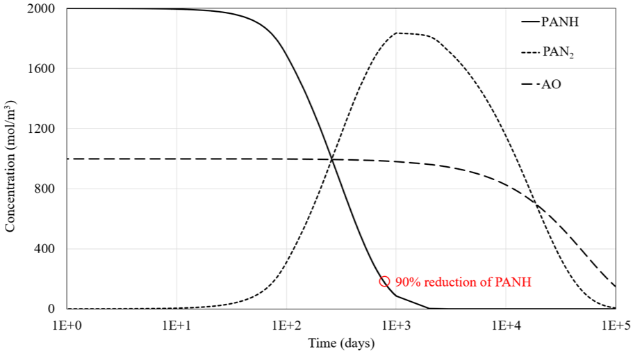
Chemical concentrations of PANH, PAN₂, and AO as function of time. The results are taken from the oil tank. Small variations are seen overall the model of ±1 mol/m³.

Parametric analysis

Next, we systematically vary parameters to determine the sensitivity of the results to these inputs.

Simulation 1: Variation of heat of combustion

This simulation involved keeping the oil flow rate (6.25E-4 m³/s) and crankshaft rotational speed (3000 rpm) constant while varying the heat of combustion (4.00E+5, 5.00E+5, 6.00E+5, 7.00E+5, and 8.00E+5 W/m²). Figure 15 shows the temperature profiles of the piston for different heat of combustion values. The oil enters at a temperature of 57°C and exits at 152°C for the lowest heat of combustion, with the exit temperature increasing to 237°C for the highest heat of combustion.

Figure 15.

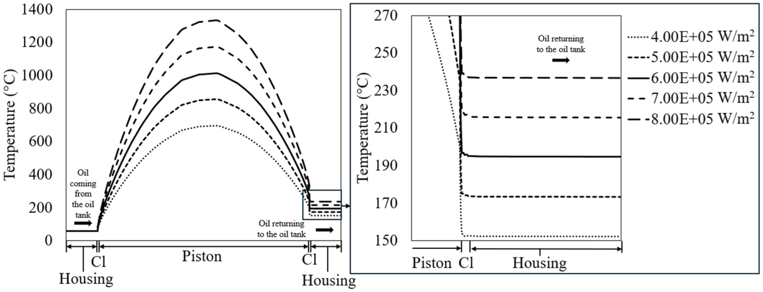
Temperature profiles of the piston at varying heat of combustion values. The oil enters at approximately the same temperature but exits the piston at higher temperatures as the heat of combustion increases.

Figure 16(b) shows the chemical concentration of PANH in the oil for different heat of combustion values. The lifespan of the oil is optimal at 5.00E+5 W/m² and reaches a minimum at 7.00E+5 W/m². Although an optimal performance was expected at 4.00E+5 W/m² and higher degradation at 8.00E5 W/m², the viscosity of the oil is highly sensitive to temperature. This sensitivity alters the flow rate and leads to deviations from the anticipated degradation trend. The results demonstrate how a single operating parameter can trigger complex fluid behavior, changing viscosity and flow resistance within system components and ultimately producing unexpected outcomes such as identical oil lifespans at two distinct heat flux values (e.g. 6.00E+5 and 8.00E+5 W/m²).

Figure 16.

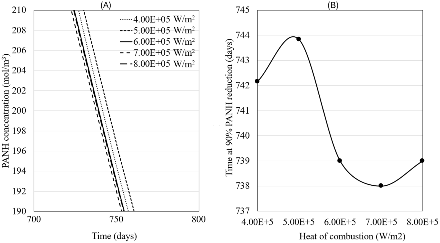
PANH chemical concentration for the different values of heat of combustion. Longer periods of time are achieved at lower heat of combustion values and shorter periods are observed as the heat of combustion is increased: (A) PANH concentration as function of time, (B) Number of days it takes to reduce 90% of PANH as function of heat of combustion.

Simulation 2: Variation of rotational speed of the journal

This simulation involved keeping the oil flow rate (6.25E-4 m³/s) and heat of combustion (6.00E+5 W/m²) constant while varying the crankshaft rotational speed (2000, 2500, 3000, 3500, and 4000 rpm). Figure 17 shows the oil temperature at the exit of the main journal bearing and the connecting rod journal bearing for different crankshaft rotational speeds. The temperature increases with higher rotational speeds, following the typical forced convection behavior reported by Khabari. ³⁵ As the flow speed increases, the convective heat transfer coefficient also increases, allowing the oil to absorb more heat from the hot surface in contact with the flow.

Figure 17.

Temperature of the oil at the exit from the main journal bearing and the connecting journal bearing at different rotational speeds.

Figure 18(b) shows the PANH chemical degradation for different crankshaft rotational speeds. Although a shorter oil lifespan would typically be expected at higher rotational speeds due to increased oil temperature, the flow speed also rises with higher rotational speeds. This increase in flow speed reduces the exposure time of the oil to the elevated temperatures, thereby limiting the extent of degradation. As a result, the oil experiences less degradation at higher rotational speeds, as observed at 3500 and 4000 rpm. The faster flow speeds cause the oil to move through the system more quickly, reducing its contact time with the high-temperature surfaces, which in turn helps preserve its chemical integrity. This behavior demonstrates the complex interplay between flow speed and temperature in influencing the degradation process, with the oil at higher speeds being exposed to the heat for shorter durations, thus mitigating the expected degradation.

Figure 18.

PANH chemical concentration for the different values of rotational speed of the crankshaft. Optimal lifespan of the oil is observed at 3000 rpm and shorter lifespan is observed at 4000 rpm: (A) PANH concentration as function of time, (B) Number of days it takes to reduce 90% of PANH as function of rotational speed of the crankshaft.

Simulation 3: Variation of the lubricant flow rate

This simulation involved keeping the heat of combustion (6.00E+5 W/m²) and crankshaft rotational speed (3000 rpm) constant while varying oil flow rate (6.00E-4, 6.25E-4, and 6.50E-4 m³/s). Figure 19 shows the temperature profiles of the piston for different oil flow rates. The oil enters at a temperature of 57°C and exits at 189°C for the highest oil flow rate, with the exit temperature increasing to 200°C for the lowest oil flow rate.

Figure 19.

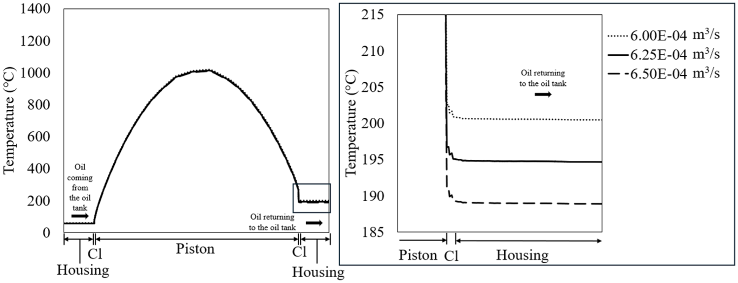
Temperature profiles for the piston at varying the oil flow rate values. The oil enters at approximately the same temperature but exits the piston at higher temperatures as the oil flow rate decreases.

Figure 20(b) shows the chemical concentration of PANH in the oil for various oil flow rate values. The lifespan of the oil is optimal at a flow rate of 6.50E-4 m³/s, where the degradation of PANH is minimized. At this flow rate, the oil maintains a more stable chemical composition, and the degradation process occurs at a slower rate. Conversely, the oil’s lifespan reaches its minimum at 6.00E-4 m³/s, where the PANH concentration decreases more rapidly.

Figure 20.

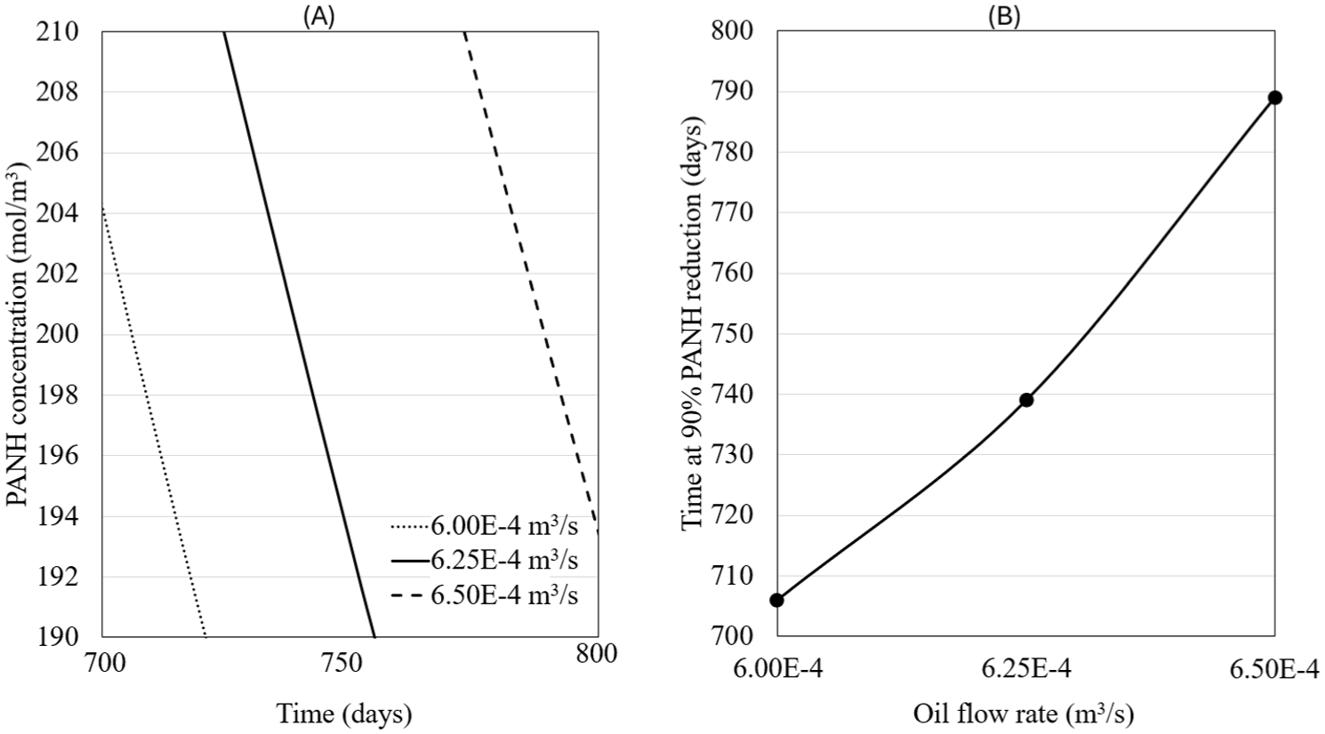
PANH chemical concentration for the different values of the oil flow rate. Optimal lifespan of the oil is observed at 6.50E-4m³/s and shorter lifespan is observed at 6.00E-4m³/s: (A) PANH concentration as function of time, (B) Number of days it takes to reduce 90% of PANH as function of oil flow rate

This behavior can be attributed to two primary factors: the reduction in temperature at the piston and the increase in flow speed as the oil flow rate rises. Higher flow rates improve the heat dissipation process, preventing excessive heat buildup at the piston and ensuring that the oil exits at lower temperatures. By keeping the oil at a lower temperature, degradation reactions are less likely to occur, significantly extending the oil’s effective lifespan. Additionally, increased flow speeds reduce the time the oil spends in contact with high-temperature areas, further reducing its exposure to degradation.

The combination of these factors creates a favorable environment for the oil to maintain its chemical stability. The optimal flow rate not only lowers the temperature but also enhances the oil’s ability to resist chemical degradation, providing longer-lasting lubrication. This highlights the importance of adjusting oil flow rates in order to balance heat management and chemical stability, ensuring the oil performs efficiently over extended operational periods.

Figure 21 summarizes the simulation results, showing the influence of key operational parameters on oil lifespan. Among the parameters analyzed, the heat of combustion shows a relatively minor impact, with only a 6 days difference between the highest and lowest predicted oil lifespans.

Figure 21.

Summary of the oil lifespan results of for the different simulations.

In contrast, the crankshaft rotational speed exerts a more pronounced effect, contributing to an 8-day variation. Higher rotational speeds generally elevate oil temperatures, accelerating degradation. However, this relationship is nonlinear: increased flow velocity at higher speeds enhances convective heat transfer, which mitigates temperature rise and reduces the duration of oil exposure to extreme temperatures.

The oil flow rate emerges as the most critical factor, with a substantial 83 days difference between the longest and shortest oil lifespans. This parameter directly influences both thermal dissipation and the residence time of the oil in high-temperature zones. Higher flow rates improve cooling efficiency and limit thermal exposure, thereby significantly extending oil service life.

To illustrate these effects, simulations were conducted for both optimal and worst-case scenarios. The optimal configuration involved a heat of combustion of 5.00E+5 W/m², a crankshaft speed of 4000 rpm, and an oil flow rate of 6.50E-4 m³/s. Conversely, the worst-case configuration employed a heat of combustion of 7.00E+5 W/m², a crankshaft speed of 3000 rpm, and an oil flow rate of 6.00E-4 m³/s.

Interestingly, the optimal parameter combination does not yield the maximum oil lifespan, highlighting the complex and nonlinear interplay between thermal loading, mechanical dynamics, and fluid flow. This underscores the necessity of a holistic optimization strategy that considers the combined influence of all operational variables.

To reduce computational demand, a simplified prediction method was evaluated using a constant oil temperature assumption. The baseline simulation results were used for comparison, selecting four representative temperature values. A temperature of 50°C, representing the minimum temperature in the tank, a temperature of 58°C, which is the average tank temperature, a temperature of 127°C, which is the temperature at which the oil exits the journal bearings, and a temperature of 154°C, which is the temperature at the piston outlet. Figure 22 presents the resulting oil lifespan predictions under these constant temperature conditions. The results clearly show the sensitivity of oil degradation to thermal exposure. A significant increase in assumed temperature from 50°C to 58°C leads to more than a 50% reduction in oil lifespan. The estimate at 58°C, representing the average oil temperature in the tank, aligns well with the full simulation results, suggesting that in practice, positioning a thermocouple within the oil tank could provide a reliable basis for degradation monitoring.

Figure 22.

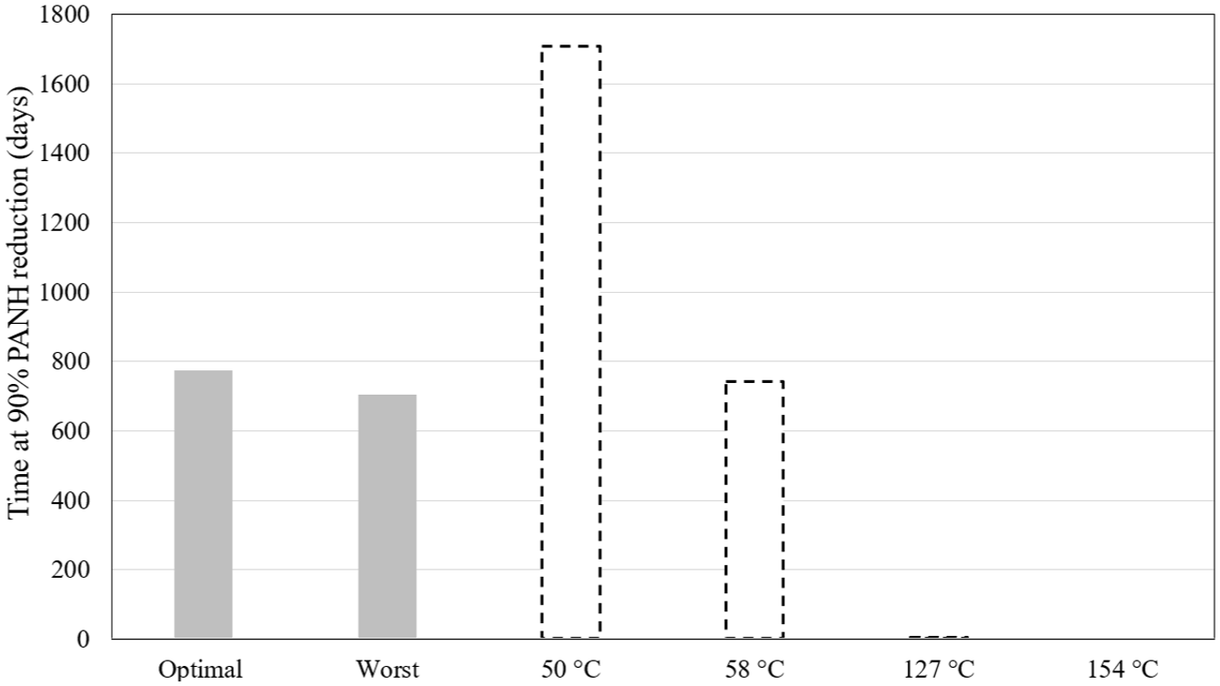
Comparison of the optimal and worst simulations with the simplified calculation of the oil degradation assuming a constant temperature.

Despite the extreme temperatures reached in engine components, these affect only small volumes of oil for brief periods. Due to the continuous flow and mixing of returning oil with cooler oil in the tank, these peak temperatures have a limited impact on overall oil degradation. The assumption of an average oil temperature in the tank effectively neglects these transient spikes, supporting its use in simplified models.

Figure 23(b) presents a comparison of PANH chemical concentration in the oil for the optimal and worst-case scenarios under a constant temperature of 58°C. The predicted values show good agreement with the more detailed simulations, reinforcing the validity of this simplified modeling approach. These findings suggest that while full-scale simulations provide precise insights, simplified methods can offer practical and computationally efficient alternatives for estimating oil degradation.

Figure 23.

Comparison of the simulations of the optimal and worst process conditions with a simplified calculation of the oil assuming a constant temperature of 58°C: (A) PANH concentration as function of time, (B) Close-up of PANH concentration as function of time

Conclusions

This study underscores the critical role that process parameters play in influencing lubricant performance and chemical degradation within maritime diesel engines. Rather than framing the problem solely in terms of selecting optimal values, the findings emphasize a deeper understanding of how each parameter affects the complex dynamics of oil lifespan. While the heat of combustion shows only a minor influence on degradation, resulting in modest variations in oil lifespan, it serves as an indicator of the thermal load of the system. In contrast, crankshaft rotational speed significantly impacts oil behavior by modulating both thermal generation and convective transport. Higher rotational speeds elevate the oil temperature due to increased friction and combustion cycles, but they simultaneously enhance oil circulation, reducing the residence time of oil in high-temperature zones and mitigating chemical degradation through improved heat dissipation.

Among all parameters studied, oil flow rate emerged as the dominant factor in controlling chemical degradation. An increased flow rate not only stabilizes the temperature within the lubrication system but also reduces the exposure of oil to critical thermal thresholds where oxidative and thermal degradation reactions become significant. The ability of the oil to cool rapidly and circulate efficiently plays a decisive role in suppressing the formation of degradation byproducts such as polyaromatic nitrated hydrocarbons (PANH).

Simulation results demonstrated that specific combinations of parameters, such the heat of combustion of 5.00E+5 W/m², a crankshaft speed of 4000 rpm, and an oil flow rate of 6.50E-4 m³/s, produced longer oil lifespans. However, the worst-case configuration, defined by a higher heat of combustion (7.00E+5 W/m²), a reduced crankshaft speed (3000 rpm), and a lower oil flow rate (6.00E-4 m³/s), led to the fastest degradation. The optimal configuration did not result in the maximum achievable lifespan, which reflects the nonlinear and coupled nature of the underlying degradation mechanisms. The relationship among thermal load, flow dynamics, and chemical kinetics is highly sensitive, and improvements in one parameter may be offset by changes in another.

Rather than seeking static optimal values, a more practical approach in real-world engine applications is to characterize the relative sensitivity and impact of each parameter on oil degradation. This knowledge can help on the design of control strategies, maintenance schedules, and even sensor placements.

Simulations performed to model a 28000-day cycle required 47 min and 56 s of computational time on a computer with 16 GB RAM and an Intel Core i9-9880H processor at 2.3 GHz. These simulations considered constant parameter values, leading to more computational stability. However, applying a continuous, real-time strategy would demand dynamic updates of operational parameters, posing both computational and logistical challenges, particularly due to the need for ongoing access to licensed commercial simulation software during the engine operation.

These results highlight that maximizing oil lifespan is less about identifying a single optimal configuration and more about understanding how operational parameters influence degradation pathways. By developing robust models that capture these dependencies, it becomes possible to simplify full-scale simulations into reduced-order prediction tools. Such models would allow for real-time monitoring and forecasting of lubricant condition, promoting both efficient engine performance and reduced maintenance demands. In essence, the study supports a shift from fixed parameter optimization toward an adaptive framework guided by predictive insights into chemical oil degradation.

This analysis was performed using material properties and kinetic data from a turbine oil. While this provides a representative demonstration of the modeling framework, its composition differs from the lubricants typically used in marine diesel engines, and the temperature regimes of those systems can be significantly different. The present model can be updated once specific thermal properties, additive composition, and oxidation kinetics of marine diesel engine oils become available. Incorporating those parameters will provide more accurate lifetime predictions that are tailored to real maritime engine applications.

The model was developed in two dimensions to ensure numerical stability and computational efficiency for this initial study. A future transition to a full three-dimensional representation is possible, but it would introduce greater complexity in the meshing of detailed components, the application of spatially varying boundary conditions, and the computational resources and time required to complete the simulations. At this stage, it remains uncertain whether a three-dimensional model would significantly improve degradation predictions without high fidelity experimental data for validation. Generating such validation data and evaluating the potential benefits of three-dimensional simulations will be part of future research efforts.