A Bayesian change point detection-based method for rolling bearing remaining useful life prediction

Abstract

Addressing the multi-stage characteristics of rolling bearing degradation with random change points, this paper proposes a novel method for predicting the Remaining Useful Life (RUL) of multi-stage degradation processes. Initially, the prior parameters of each stage model are estimated using offline historical data. Then, for a single online device, real-time change point detection is performed using the Bayesian change point detection method. The Bayesian updating approach is adopted to update the parameters of the first stage before the change point occurs and the second stage after the change point. Subsequently, the multi-stage model is utilized for RUL prediction. Numerical simulations and case studies have shown that the rolling bearing life prediction method based on Bayesian change point detection can improve change point detection accuracy by 85%, thereby achieving high-precision multi-stage RUL prediction.

Introduction

Rolling bearings, as the most common and extremely crucial rotating components in industrial equipment, are widely applied in rotating machinery such as motors, gearboxes, and turbines. Whether their operation status is normal directly affects the performance of the entire equipment.^1,2 During the operation process, due to the influence of internal factors (such as sudden changes in the degradation mechanism) or external factors (changes in load, working conditions, etc.), the degradation characteristics of rolling bearings also change accordingly, thereby multi-stage characteristics often occur.^3,4 As shown in Figure 1, three typical stages are clearly observed during the operation of this bearing: early stage—slow degradation period, middle stage—moderate degradation period, and late stage—rapid degradation period.

Figure 1.

The three-stage degradation process of rolling bearing.

The Wiener process is a type of diffusion process with a linear drift term. Due to its excellent mathematical properties, it has been widely used in equipment reliability prediction and life analysis since the 1990s.^5,6 In recent years, continuous new progress has been made. Peng and Tseng ⁷ established a cumulative degradation model, studied the degradation modeling and prediction model within a linear framework, and derived the explicit solution of the life distribution. Lee and Tang ⁸ proposed an improved EM algorithm to estimate the parameters in the degradation process. Joseph and Yu ⁹ conducted research on the nonlinear degradation model, which can be linearized under certain conditions, and they also studied the degradation modeling problem considering the data correlation. However, all the above methods utilize the historical monitoring data of the service lives of similar equipment and do not make use of the monitoring degradation data during the operation of the in-service equipment. In order to overcome this problem, Gebraeel et al. ¹⁰ proposed a stochastic degradation modeling method under the Bayesian framework. After obtaining the degradation monitoring data, the Bayesian method is used to update the stochastic parameters of the model, obtain their posterior estimates, and then predict the probability distribution of the remaining useful life. Shi and Xue ¹¹ proposed a method for predicting the remaining useful life that integrates the prior degradation data and the on-site degradation data of the equipment itself, established an equipment degradation model that conforms to the description of the nonlinear Wiener process.

Currently, there have been many studies on the degradation modeling and life prediction of equipment with typical multi-stage degradation characteristics.^12,13 Ng ¹⁴ proposed a two-stage independent increment degradation model with independent increments based on a single change point. Wang et al. ¹⁵ proposed a two-stage bearing degradation modeling combining the EM algorithm and Kalman filter for adaptive prediction. Dong et al. ¹⁶ proposed a method for predicting the Remaining Useful Life (RUL) based on a two-stage adaptive Wiener process. For the degradation modeling of multi-stage processes, the key lies in accurately detecting the points where the degradation rules change, that is, the change points. ¹⁶ For the typical three-stage bearing degradation process, generally, the time point of the occurrence of the second stage is taken as the initial fault point, which is also called the First Prediction Time (FPT), and the degradation process modeling is carried out with the subsequent two stages (the middle and late stages) as the targets. Figure 2 shows the typical two-stage degradation process of a rolling bearing. Under the condition of determining the failure threshold, its real life is point A in the figure. At present, the main problems existing in the real-time online life prediction of the multi-stage degradation process are as follows:

Figure 2.

Error analysis of RUL based on two-stage degradation process.

If the change points in the degradation process are not taken into account, that is, the process is regarded as a single process, it will lead to a very large prediction error. For example, in Figure 2, the predicted life at point A1 has a huge gap from the real life at point A.

When considering the change points and treating the process as a two-stage process, the prediction accuracy of the change points is very important. For example, in Figure 2, owing to the prediction error of the change points, the estimated life prediction point is located at point A2, resulting in a large error.

At the same time, the current multi-stage degradation modeling and prediction are not suitable for online life prediction, real-time change point detection and real-time remaining useful life prediction cannot be carried out.

Statistical change point analysis theory, which focuses on modeling abrupt changes in real-world processes, is a nonlinear statistical framework that has witnessed substantial advancements in both theoretical development and practical applications in recent years.^13,15,16

Current mainstream methodologies for change point detection include the Pettitt method, ¹⁷ Bayesian testing approaches, ¹⁸ and the cumulative sum (CUSUM) test. ¹⁹ The Pettitt, a nonparametric approach for change-point detection, examines the relative ranks of all pairwise comparisons within the time series. This distribution-free method is particularly valuable as it requires no prior knowledge of the underlying data distribution and maintains robustness across different time series types. However, the Pettitt test exhibits certain drawbacks, including reduced accuracy in identifying multiple change-points and heightened sensitivity to both the time series length and the position of the change point(s). ¹⁷ The CUSUM test, on the other hand, requires a large dataset to construct test statistics, which limits its accuracy when applied to small sample sizes. In contrast, Bayesian change point detection methods, under appropriate prior assumptions, can effectively identify change points with relatively high precision while meeting the requirements for real-time detection capabilities.

In response to the above analysis, this paper proposes a novel adaptive change point detection-based RUL prediction method for bearing degradation models. First, parameter learning is conducted using historical data to determine the prior values of change point distribution patterns, followed by the estimation of drift and diffusion coefficients for different stages. By applying change point detection to the collected degradation observation data, the observation sequence is partitioned into multiple segments. Starting from the FPT, online life prediction is performed. Both simulation experiments and real-world case studies validate the prediction accuracy and practical applicability of the proposed method.

Problem description

Let $X(t)$ represent the performance degradation amount of a rolling bearing at time $t$ . If a change point $\tau$ exists in the degradation process, $x_0$ denotes the initial value of the degradation process. Divide the degradation sequence into two different stages $x_0^{\tau }$ , $x_{\tau +1}^n$ with the change point $\mathrm{\tau }$ , and the corresponding degradation parameters are ${\theta }^{(1)}$ and ${\mathrm{\theta }}^{(2)}$ (the specific parameters depend on the established model). Let the failure threshold be $\omega$ , and the equipment life $T_{\omega }$ ²⁰ :

$$T_{\omega }=\inf \{t:X(t)\ge \omega |x_0<\omega \}$$

(1)

Let $t$ denote the current time, and let $x_0^k$ represent the acquired real-time degradation sequence. Consequently, the remaining life corresponding to time $t_k$ can be denoted as:

$$L_k=\inf \{l_k:X(l_k+t_k)\ge \omega |X(t_k)<\omega \}$$

(2)

The tasks of real-time online life prediction are: Estimate the current change-point $\mathrm{\tau }$ and the model parameters ${\mathrm{\theta }}^{(1)}$ and ${\mathrm{\theta }}^{(2)}$ before and after the change-point in real-time; Considering two cases of $t_k\le \tau$ and $t_k>\tau$ , estimate the remaining life $l_k$ of the current time $t_k$ .

Two-stage degradation process model

For the typical three-stage rolling bearing degradation process, since the first stage operates smoothly, remaining life prediction is generally not performed. This paper establishes a two-stage degradation process model focusing on the latter two stages of rolling bearings. The following assumptions are made:

The rolling bearing degradation process starts from the FPT, with all prediction objects having two typical degradation stages, namely the moderate degradation stage (Stage 1) and the rapid degradation stage (Stage 2); Each stage is a linear Wiener process.

Two-stage Wiener linear model

Based on the above assumptions, the studied degradation process model is expressed as:

$$X(t)=\{\begin{array}{c}{x}_0+{\mu }_{1}t+{\sigma }_{1}B(t)\hfill \\ \multicolumn{1}{c}{x_{\tau }+{\mu }_2(t-\tau )+{\sigma }_{2}B(t-\tau )}\end{array}\begin{array}{c}0<t\le \tau \hfill \\ \multicolumn{1}{c}{\tau <t}\end{array}$$

(3)

In the formula, $\mu =[{\mu }_1,{\mu }_2],\sigma =[{\sigma }_1,{\sigma }_2]$ represents the drift coefficient and diffusion coefficient for stages 1 and 2, respectively. $\tau$ and $x_{\tau }$ represent the occurrence time of the change points and the corresponding degradation amounts, respectively. $x_0$ is the initial deterioration amount of the device, which is generally set to 0, and $B\left(t\right)$ represents standard Brownian motion. The randomness of Brownian motion is used to reflect the uncertainty in the prediction of remaining life.

The RUL distribution of the two-stage degradation process

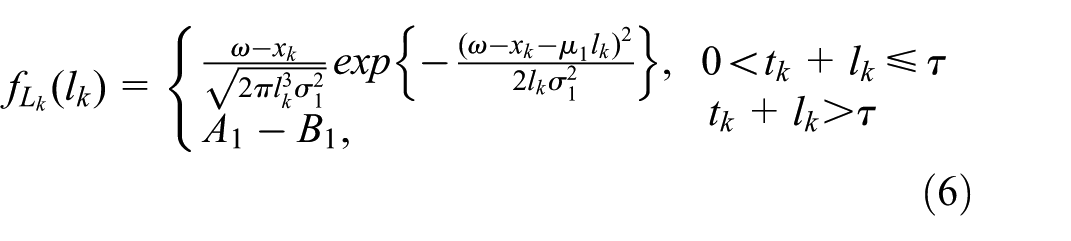
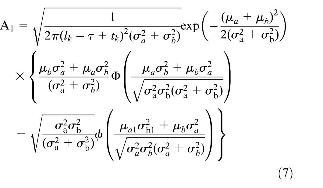
Based on the above assumptions, the RUL Probability Density Function (PDF) of the two-stage degradation process model studied in this paper can be expressed as ²⁰ :

$$f(t)=\{\begin{array}{c}\frac{\omega -x_0}{\sqrt{2\pi t^3{\sigma }_1^2}}\exp (A_0)\hfill \\ \multicolumn{1}{c}{{\int }_{-\infty }^{\omega }\frac{\omega -x_{\tau }}{\sqrt{2\pi {(t-\tau )}^3{\sigma }_2^2}}\exp (B_0)g_{\tau }(x_{\tau })d{x}_{\tau }}\end{array}\begin{array}{c}0<t\le \tau \hfill \\ \multicolumn{1}{c}{\tau <t}\end{array}$$

(4)

Where ${\mathrm{A}}_0=-\frac{{(\omega -x_0-{\mu }_{1}t)}^2}{2t{\sigma }_1^2}$ , ${\mathrm{B}}_0=-\frac{{(\omega -x_{\tau }-{\mu }_2(t-\tau ))}^2}{2(t-{\tau }_1){\sigma }_2^2}$ , $g_{\tau }\left(x_{\tau }\right)$ represent the transition probability ²⁰ of transitioning from 0 to $x_{\tau }$ over time $\tau$ , and its expression is:

$$\begin{array}{c}\multicolumn{1}{c}{g_{\tau }(x_{\tau })=\frac{1}{\sqrt{2\pi \tau {\sigma }_1^2}}\{\exp [-\frac{{(x_{\tau }-{\mu }_1\tau )}^2}{2\tau {\sigma }_1^2}]}\end{array}-\exp \left(\frac{2{\mu }_1\omega }{{\sigma }_1^2}\right)\exp [-\frac{{(x_{\tau }-2\omega -{\mu }_1\tau )}^2}{2\tau {\sigma }_1^2}]\}$$

(5)

The PDF at time $t_k$ is ²⁰ :

$$f_{L_k}(l_k)=\{\begin{array}{c}\frac{\omega -x_k}{\sqrt{2\pi l_k^3{\sigma }_1^2}}\exp \{-\frac{{(\omega -x_k-{\mu }_1{l}_k)}^2}{2l_k{\sigma }_1^2}\},\hfill \\ \multicolumn{1}{c}{A_1-B_1,}\end{array}\begin{array}{c}0<t_k+l_k\le \tau \hfill \\ \multicolumn{1}{c}{t_k+l_k>\tau }\end{array}$$

(6)

Where

$$\begin{array}{c}\multicolumn{1}{c}{{\mathrm{A}}_1=\sqrt{\frac{1}{2\pi {(l_k-\tau +t_k)}^2({\sigma }_a^2+{\sigma }_b^2)}}\exp (-\frac{{({\mu }_a+{\mu }_b)}^2}{2({\mathrm{\sigma }}_{\mathrm{a}}^2+{\mathrm{\sigma }}_{\mathrm{b}}^2)})}\\ \multicolumn{1}{c}{\times \{\frac{{\mu }_b{\sigma }_a^2+{\mu }_a{\sigma }_b^2}{({\sigma }_a^2+{\sigma }_b^2)}\mathrm{\Phi }\left(\frac{{\mu }_a{\sigma }_b^2+{\mu }_b{\sigma }_a^2}{\sqrt{{\mathrm{\sigma }}_{\mathrm{a}}^2{\mathrm{\sigma }}_{\mathrm{b}}^2({\mathrm{\sigma }}_{\mathrm{a}}^2+{\mathrm{\sigma }}_{\mathrm{b}}^2)}}\right)}\\ \multicolumn{1}{c}{+\sqrt{\frac{{\mathrm{\sigma }}_{\mathrm{a}}^2{\mathrm{\sigma }}_{\mathrm{b}}^2}{({\mathrm{\sigma }}_{\mathrm{a}}^2+{\mathrm{\sigma }}_{\mathrm{b}}^2)}}\varphi \left(\frac{{\mu }_{a1}{\mathrm{\sigma }}_{\mathrm{b}1}^2+{\mu }_b{\sigma }_a^2}{\sqrt{{\sigma }_a^2{\sigma }_b^2({\sigma }_a^2+{\sigma }_b^2)}}\right)\}}\end{array}$$

(7)

$$\begin{array}{l}{B}_1=exp\left\{\frac{2{\mu }_{1P}(\omega -x_k)}{{\sigma }_1^2}+\frac{2[{(\omega -x_k)}^2{\sigma }_{1P}^4\tau +{(\omega -x_k)}^2{\sigma }_{1P}^2{\sigma }_1^2]}{[{\sigma }_1^2+(\tau -l_k){\sigma }_{1P}^2]{\sigma }_1^4}\right\}\\ \times \frac{exp(-2\frac{{({\mu }_a-{\mu }_b)}^2}{({\sigma }_a^2+{\sigma }_b^2)})}{2\pi {(l_k-\tau +t_k)}^2({\sigma }_a^2+{\sigma }_b^2)}\\ \times \left\{\frac{{\mu }_c{\sigma }_a^2+{\mu }_a{\sigma }_b^2}{({\sigma }_a^2+{\sigma }_b^2)}\Phi \left(\frac{{\mu }_a{\sigma }_b^2+{\mu }_b{\sigma }_a^2}{\sqrt{{\sigma }_a^2{\sigma }_b^2({\sigma }_a^2+{\sigma }_b^2)}}\right)+\sqrt{\frac{{\sigma }_a^2{\sigma }_b^2}{({\sigma }_a^2+{\sigma }_b^2)}}\varphi \left(\frac{{\mu }_c{\sigma }_a^2+{\mu }_a{\sigma }_b^2}{\sqrt{{\sigma }_a^2{\sigma }_b^2({\sigma }_a^2+{\sigma }_b^2)}}\right)\right\}\end{array}$$

(8)

$\mathrm{\Phi }(·)$ is the cumulative distribution function of the standard normal distribution, $\varphi (·)$ is the probability density function of the standard normal distribution.

Where ${\mu }_a={\mu }_{2P}(l_k-\tau +t_k)$ , ${\mu }_b=\omega -x_k-{\mu }_{1P}(\tau -t_k)$ , ${\mu }_c=-\omega +x_k-{\mu }_{1P}(\tau -t_k)-2\omega (\tau -l_k){\sigma }_{1P}^2/{\sigma }_1^2$ , ${\sigma }_a^2={\sigma }_2^2(l_k-\tau +t_k)+{\sigma }_{2P}^2(l_k-\tau +t_k{)}^2,{\sigma }_b^2={\sigma }_1^2(\tau -t_k)+{\sigma }_{1P}^2(\tau -t_k{)}^2$ .

Offline parameter estimation

Considering that there are a total of $\mathrm{n}$ rolling bearings in the same batch, there are $\mathrm{n}$ sets of degradation data, namely $X=[x_1,x_2,\dots ,x_n]$ , where $x_i=[x_{i,0},x_{i,1},x_{i,2},\dots ,x_{i,m_i}]$ represents the monitoring value of the $\mathrm{i}$ -th bearing at time $[t_{i,0},t_{i,1},t_{i,2},\dots ,t_{i,m_i}]$ , and $m_i$ is the number of monitoring values for the $\mathrm{i}$ -th bearing. Let different bearings collect their degradation data at equal intervals, namely $\mathrm{\Delta }t=t_{i,j}-t_{i,j-1}$ . Assume that the parameters ${\mu }_1$ and ${\mu }_2$ of the two stages follow Gaussian distributions $N({\mu }_{1P},{\sigma }_{1P}^2)$ and $N({\mu }_{2P},{\sigma }_{2P}^2)$ , and the change point ${\tau }_i$ follows the $\mathrm{Gamm}(\alpha ,\beta )$ distribution, with shape parameter and scale parameter being $\mathrm{\alpha }$ and $\mathrm{\beta }$ respectively. ²⁰

Using MLE (Maximum Likelihood Estimation) to estimate its parameters, first let ${\tau }_i$ be the change point of device $\mathrm{i}$ , and construct the likelihood function as shown in equation (9):

$$\begin{array}{c}\mathrm{lnL}({\mu }_{1,i},{\sigma }_1,{\mu }_{2,i},{\sigma }_2,{\tau }_i|x_i)\hfill \\ \multicolumn{1}{c}{=\sum _{j=1}^{{\tau }_i}\ln \frac{1}{{\sigma }_1\sqrt{2\pi \mathrm{\Delta }t}}\exp [-\frac{{(x_{i,j}-x_{i,j-1}-{\mu }_{1,i}\mathrm{\Delta }t)}^2}{2\mathrm{\Delta }t{\sigma }_1^2}]}\\ \multicolumn{1}{c}{+\sum _{j={\tau }_i+1}^{m_i}\ln \frac{1}{{\sigma }_2\sqrt{2\pi \mathrm{\Delta }t}}\exp [-\frac{{(x_{i,j}-x_{i,j-1}-{\mu }_{2,i}\mathrm{\Delta }t)}^2}{2\mathrm{\Delta }t{\sigma }_2^2}]}\end{array}$$

(9)

The maximum likelihood estimate of parameter ${\hat{\Theta }}_i=({\hat{\mu }}_{1,i},{\hat{\mu }}_{2,i},{\hat{\sigma }}_1^2,{\hat{\sigma }}_2^2,{\hat{\tau }}_i),i=1,2,\dots ,n$ is ²⁰ :

$${\hat{\Theta }}_i=\underset{\Theta }{\mathrm{argmax}}\mathrm{lnL}({\mu }_{1,i},{\sigma }_1,{\mu }_{1,i},{\sigma }_2,{\tau }_i|x_i)$$

(10)

Using the values of ${\hat{\theta }}_i$ from multiple devices, the estimate of ${\sigma }_1,{\sigma }_2,{\mu }_{1P},{\mu }_{2P},\tau$ can be obtained.

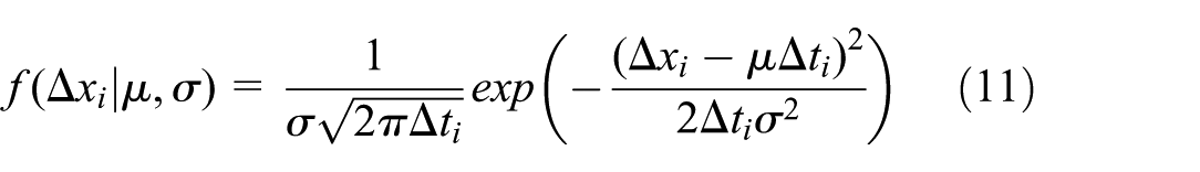
The PDF of degradation increments

For the standard Wiener process $x_0^n=[x_0,x_1,x_2,\dots ,x_n]$ , define its increment sequences, $\mathrm{\Delta }{x}_1^n=[\mathrm{\Delta }{x}_1,\mathrm{\Delta }{x}_2,\dots ,\mathrm{\Delta }{x}_n],\mathrm{\Delta }{x}_i=x_i-x_{i-1}$ , $\mathrm{\Delta }{t}_i=t_i-t_{i-1},i=1,2,\dots n$ . $\mathrm{\Delta }{x}_i$ and $\mathrm{\Delta }{t}_i$ are the performance degradation increments and time increments, respectively. It can be inferred from the normality of the Wiener process that $\mathrm{\Delta }{x}_i~N(\mu \mathrm{\Delta }{t}_i,{\sigma }^2\mathrm{\Delta }{t}_i)$ .

Then PDF of $\mathrm{\Delta }{x}_i$ is:

$$f(\mathrm{\Delta }{x}_i|\mu ,\sigma )=\frac{1}{\sigma \sqrt{2\pi \mathrm{\Delta }{t}_i}}\exp (-\frac{{(\mathrm{\Delta }{x}_i-\mu \mathrm{\Delta }{t}_i)}^2}{2\mathrm{\Delta }{t}_i{\sigma }^2})$$

(11)

Here, the prior distribution of $\theta =(\mu ,{\sigma }^2)$ is a normal-inverse gamma distribution, ²¹ that is, $\theta ~N/\mathrm{IGa}(m,v,a,B)$ .

If the hyperparameters (m, v, a, B) are defined, then:

$$\begin{array}{c}\multicolumn{1}{c}{p(\theta |m,v,a,B)=\exp \{-\frac{v{\mu }^2}{2{\sigma }^2}+\frac{\mathrm{vm}\mu }{{\sigma }^2}-\frac{B}{{\sigma }^2}+\frac{v{m}^2}{{\sigma }^2}}\end{array}+(a-\frac{1}{2})\ln \frac{1}{{\sigma }^2}-\ln Z_{\mathrm{NIG}}(\eta )\}$$

(12)

where $Z_{\mathrm{NIG}}\left(\eta \right)={(2\pi /v)}^{1/2}{\left|B\right|}^{-a}\Gamma \left(a\right)$ , $\Gamma \left(a\right)$ is the gamma function.

Bayesian change point detection

Bayesian change point detection is an online change point detection algorithm, ¹⁸ determining whether a change point $t_c$ has occurred by generating an accurate distribution of the next unseen data in the sequence from the observed data. The increment degradation sequence $\mathrm{\Delta }{x}_1^n$ introduced in Section “Two-stage degradation process model” is used for change point detection.

Change point detection method

Bayesian change point detection models the run length $r_t$ starting from the last change point, ¹⁸ $r_t=[r_{1t},r_{2t},\dots r_{\mathrm{kt}},\dots r_{\mathrm{tt}},{]}^T$ ., with $1\le k\le t,r_{\mathrm{kt}}=1$ indicating the moment $k$ as a change point. Given that the run length for any moment (t−1) is $r_{t-1}$ , the run length $r_t$ at the next moment $t$ can take only two values: when the sequence continues to grow according to the original distribution, the length of the sequence $r_t=r_{t-1}+1$ ; when a change point occurs at moment $t$ , $r_t=1$ .

The probability that the degradation pattern of the device changes (i.e. a change point $r_t=1$ occurs) is $H\left(r_t\right)$ , and when the duration of the degradation pattern follows a certain distribution, $H\left(r_t\right)$ is the hazard function of that distribution, then ¹⁸ :

$$p(r_t\mid r_{t-1})=\{\begin{array}{cc}1-H(r_{t-1}+1),\hfill & r_t=1\hfill \\ \multicolumn{1}{c}{H(r_{t-1}+1),}& r_t=r_{t-1}+1\hfill \\ \multicolumn{1}{c}{0,}& \mathrm{other}\hfill \end{array}$$

(13)

Among them, $H\left(\tau \right)=\frac{P_{\mathrm{qap}}(g=\tau )}{\sum _{t=\tau }^{\infty }{P}_{\mathrm{qap}}(g=t)}$ is its risk function, ¹⁸ in the special case is where $P_{\mathrm{qap}}\left(g\right)$ is a discrete exponential distribution with timescale $\mathrm{\lambda }$ , the process is memoryless and the hazard function is constant at $H\left(\tau \right)=1/\mathrm{\lambda }$ .

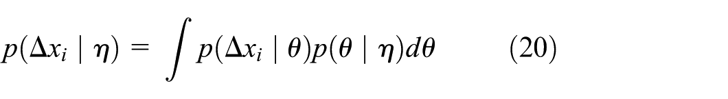
According to the given variable length $r_t$ , the marginal probability summation shows:

$$p(\mathrm{\Delta }{x}_{t+1}\mid \mathrm{\Delta }{x}_1^t)=\sum _{r_t}p(\mathrm{\Delta }{x}_{t+1}\mid r_t,\mathrm{\Delta }{x}_k^t)p(r_t\mid \mathrm{\Delta }{x}_1^t)$$

(14)

Here, $\mathrm{\Delta }{x}_k^t$ represents the nearest $(r_t=t-k+1)$ associated observation points $\mathrm{\Delta }{x}_k,\mathrm{\Delta }{x}_{k+1},\dots \mathrm{\Delta }{x}_{t-1},\mathrm{\Delta }{x}_t$ at time $t$ . The posterior probability $p(r_t\mid \mathrm{\Delta }{x}_1^t)$ here is:

$$p(r_t\mid \mathrm{\Delta }{x}_1^t)=\frac{p(r_t,\mathrm{\Delta }{x}_1^t)}{p\left(\mathrm{\Delta }{x}_1^t\right)}$$

(15)

The joint probability $\mathrm{p}({\mathrm{r}}_{\mathrm{t}},\mathrm{\Delta }{\mathrm{x}}_1^{\mathrm{t}})$ can be expressed in a recursive form:

$$\begin{array}{c}\multicolumn{1}{c}{p(r_t,\mathrm{\Delta }{x}_1^t)=\sum _{r_{t-1}}p(r_t,r_{t-1},\mathrm{\Delta }{x}_1^t)}\\ \multicolumn{1}{c}{=\sum _{r_{t-1}}p(r_t\mid r_{t-1})p(\mathrm{\Delta }{x}_t\mid r_{t-1},\mathrm{\Delta }{x}_k^t)p(r_{t-1},\mathrm{\Delta }{x}_1^{t-1})}\end{array}$$

(16)

From equations (20). and (21), we obtain the recursive formula for posterior probability of $p(r_t\mid \mathrm{\Delta }{x}_1^t)$ ¹⁸ :

$$p(r_t\mid \mathrm{\Delta }{x}_1^t)=\sum _{r_{t-1}}p(\mathrm{\Delta }{x}_t\mid r_t,\mathrm{\Delta }{x}_k^t)p(r_t\mid r_{t-1})p(r_{t-1}\mid \mathrm{\Delta }{x}_1^{t-1})$$

(17)

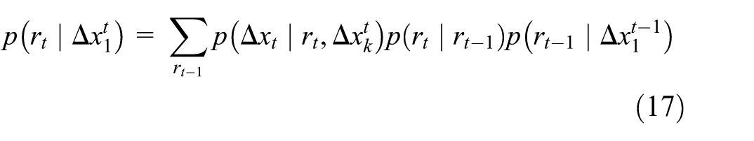
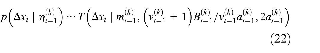
Note that, according to the properties of conditional independence, the predictive distribution $p(\mathrm{\Delta }{x}_t\mid r_{t-1},\mathrm{\Delta }{x}_1^t)$ depends only on the most recent data $\mathrm{\Delta }{x}_k^t$ , and uses the properties of the conjugate exponential distribution family for simplified calculations.

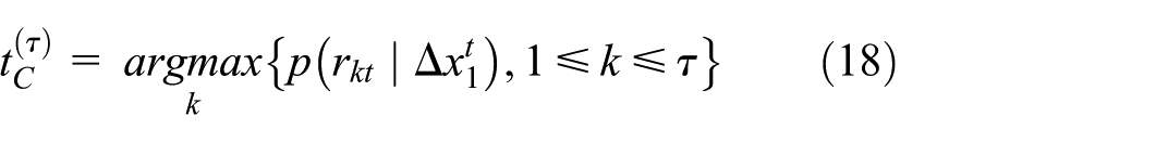
According to equation (22), the current time $\tau$ corresponds to the change point $t_C^{\left(\tau \right)}$ ²¹ :

$$t_C^{\left(\tau \right)}=\underset{k}{\mathrm{argmax}}\{p(r_{\mathrm{kt}}\mid \mathrm{\Delta }{x}_1^t),1\le k\le \tau \}$$

(18)

Conjugate exponential distribution

For the convenience of calculation, assume that the degenerate increment $\mathrm{\Delta }{x}_i$ is generated by an exponential distribution family with a conjugate prior distribution. ¹⁸ The prior distribution $p(\theta \mid \eta )$ and posterior distribution $p(\theta \mid \mathrm{\Delta }{x}_i)$ of parameter $\theta$ have the same form, and the hyperparameters satisfy the following relationship.

$${\eta }_{\mathrm{post}}=\eta +\sum _{t=1}^{n}u\left(\mathrm{\Delta }{x}_i\right)$$

(19)

The likelihood function form of the exponential distribution is:

$$p(\mathrm{\Delta }{x}_i\mid \eta )=\int p(\mathrm{\Delta }{x}_i\mid \theta )p(\theta \mid \eta )d\theta$$

(20)

The calculated marginal distribution is a $\mathrm{T}$ distribution, that is: $\mathrm{\Delta }{x}_i\mid \eta ~T(\mathrm{\Delta }{x}_i\mid m,(v+1)B/\mathrm{va},2a)$ Taking $\mathrm{\phi }\left(\mathrm{\theta }\right)=[-{\mathrm{u}}^2/2{\mathrm{\sigma }}^2,\mathrm{u}/{\mathrm{\sigma }}^2,1/{\mathrm{\sigma }}^2,-\log {\mathrm{\sigma }}^2],\eta =[v,\mathrm{vm},B+v{m}^2/2,a-1/2],\phi \left(\theta \right)$ and $\eta$ as the sufficient statistics and hyperparameters respectively, and $u\left(\mathrm{\Delta }{x}_i\right)=[1,\mathrm{\Delta }{x}_i,\mathrm{\Delta }{x_i}^2/2,1/2]$ . The recursive formula for the posterior hyperparameter is obtained as:

$$\{\begin{array}{cc}{v}_{t+1}=v_t+1,\hfill & B_{t+1}=B_t+\frac{v_t{(m_t-\mathrm{\Delta }{x}_{t+1})}^2}{2(v_t+1)}\hfill \\ \multicolumn{1}{c}{a_{t+1}=a_t+\frac{1}{2},}& m_{t+1}=\frac{v_t{m}_t+\mathrm{\Delta }{x}_{t+1}}{v_t+1}\hfill \end{array}$$

(21)

Thus, the recursive formula for the predicted distribution probability $p(\mathrm{\Delta }{x}_t\mid {\eta }_{t-1}^{\left(k\right)})$ can be obtained:

$$\begin{array}{c}\multicolumn{1}{c}{p(\mathrm{\Delta }{x}_t\mid {\eta }_{t-1}^{\left(k\right)})~T(\mathrm{\Delta }{x}_t\mid m_{t-1}^{\left(k\right)},(v_{t-1}^{\left(k\right)}+1)B_{t-1}^{\left(k\right)}/v_{t-1}^{\left(k\right)}{a}_{t-1}^{\left(k\right)},2a_{t-1}^{\left(k\right)})}\end{array}$$

(22)

In the equation, ${\eta }_{t-1}^{\left(k\right)}$ represents the posterior distribution hyperparameters calculated based on $\mathrm{\Delta }{x}_k^t$ .

Bayesian change point detection algorithm

Algorithm 1: Bayesian Change Point Detection Algorithm:

• Step 1: Initialize $p\left(r_1\right)=1$ , determine its offline parameter estimation using equation (10) based on offline data, and use the offline parameter to estimate its hyperparameters value $m_0,v,a_0,B_0$ ;

• Step 2: Obtain a new set of degraded incremental data $\mathrm{\Delta }{x}_t$ ;

• Step 3: Calculate the predicted distribution probability ${\pi }_t^{\left(r_t\right)}=p(\mathrm{\Delta }{x}_t\mid {\eta }_t^{\left(k\right)})$ for $\mathrm{\Delta }{x}_t$ according to equation (22);

• Step 4: Calculate the growth probability $p(r_t=r_{t-1}+1,\mathrm{\Delta }{x}_1^t)$ for $(r_t=r_{t-1}+1)$ according to equation (17);

• Step 5: Calculate the change point probability $p(r_t=1,\mathrm{\Delta }{x}_1^t)$ for $(r_t=1)$ according to equation (17);

• Step 6: Calculate the evidence $p\left(\mathrm{\Delta }{x}_1^t\right)=\sum _{r_t}p(r_t,\mathrm{\Delta }{x}_1^t)$ using integration according to equation (14);

• Step 7: Determine the posterior distribution $p(r_t\mid \mathrm{\Delta }{x}_1^t)=p(r_t,\mathrm{\Delta }{x}_1^t)/p\left(\mathrm{\Delta }{x}_1^t\right)$ of runtime $r_t$ ;

• Step 8: Determine the change point according to equation (18) $t_C^{\left(t\right)}$ ;

• Step 9: Update the hyperparameters according to equation (21), switch to Step 2.

Bayesian change point detection based RUL prediction

RUL prediction flowchart

Figure 3 illustrates the flowchart of the Bayesian change point detection-based RUL prediction method for rolling bearings. The process begins with offline historical data from multiple homogeneous bearings to construct a multi-stage degradation model, where prior parameters are estimated via maximum likelihood estimation (MLE).

Figure 3.

Flowchart of Bayesian change point detection-based RUL prediction.

For online prediction, real-time monitoring data from a target bearing is used to compute degradement increments. The Bayesian framework then evaluates whether a change point (e.g. degradation stage transition) occurs by calculating posterior probabilities and separating growth and change point probabilities. If detected, model parameters are updated in real-time. Finally, the RUL is predicted as a PDF based on the first passage time of the degradation trajectory crossing a failure threshold. This approach integrates offline learning with online adaptation, enhancing RUL prediction accuracy for rolling bearings.

Online parameter update

For real-time RUL prediction of a single rolling bearing, to fully utilize the online collected data, Bayesian theory can be employed for online parameter updating, with the bearing monitoring at the current time $t_k$ , and the collected data from time 1 to $t_k$ being $x_1^k$ .

Let ${\Theta }_0=[{\mu }_{1,0},{\sigma }_{1,0},{\mu }_{2,0},{\sigma }_{2,0},\tau ]$ be the prior information learned offline. Let the current device change point be $\tau$ . When $t_k<\tau$ , it indicates that the device is in the first degradation stage, and there is no degradation data for the second stage yet, thus the model parameters for the first stage $({\mu }_{1P,0},{\sigma }_{1P,0})$ can be updated at this point. If $t_k>\tau$ , then the change point has occurred, requiring only the update of the second stage parameters $({\mu }_{2P},{\sigma }_{2P})$ .

When $t_k<\tau ,\Theta ~N({\mu }_{1P,0},{\sigma }_{1P,0}^2)$ , the posterior estimation of $\Theta ,p\left(\Theta \mid x_1^k\right)$ is computed as follows:

$$p({\mu }_1\mid x_1^k)=\frac{1}{{\sigma }_{1P,0}\sqrt{2\pi }}\exp \left\{\frac{{({\mu }_1-{\mu }_{1P})}^2}{2{\sigma }_{1P}^2}\right\}$$

(23)

Where,

$$\{\begin{array}{c}{\mu }_{1P}=\frac{{\mu }_{1P,0}{\sigma }_1^2+(x_k-x_0){\sigma }_{1P,0}^2}{(t_k-t_0){\sigma }_{1P,0}^2+{\sigma }_1^2}\hfill \\ \multicolumn{1}{c}{{\sigma }_{1P}^2=\frac{{\sigma }_1^2{\sigma }_{1P,0}^2}{(t_k-t_0){\sigma }_{1P,0}^2+{\sigma }_1^2}}\end{array}$$

(24)

When $t_k>\tau$ , only the parameters of $p({\mu }_2\mid x_1^k)$ need to be updated ²⁰ :

$$p({\mu }_2\mid x_{\tau }^k)=\frac{1}{{\sigma }_{2P,0}\sqrt{2\pi }}\exp \left\{\frac{{({\mu }_2-{\mu }_{2P})}^2}{2{\sigma }_{2P}^2}\right\}$$

(25)

Where

$$\{\begin{array}{c}{\mu }_{2P}=\frac{{\mu }_{2P,0}{\sigma }_2^2+(x_k-x_{\tau }){\sigma }_{2P,0}^2}{(t_k-t_{\tau }){\sigma }_{2P,0}^2+{\sigma }_2^2}\hfill \\ \multicolumn{1}{c}{{\sigma }_{2P}^2=\frac{{\sigma }_2^2{\sigma }_{2P,0}^2}{(t_k-t_{\tau }){\sigma }_{2P,0}^2+{\sigma }_2^2}}\end{array}$$

(26)

RUL prediction algorithm

Algorithm 2: Multi-stage Degradation RUL Prediction Algorithm:

• Step 1: Based on multiple sets of historical data, use equation (10) to determine the prior distribution of the hyperparameters where the common parameters (including change point $\tau$ ) have a distribution of ${\sigma }_1,{\sigma }_2,{\mu }_{1P},{\mu }_{2P},\tau$ as $\mathrm{Gamm}(\alpha ,\beta )$ .

• Step 2: For a specific degrading device, observe the latest data $x_k$ at the current time $t_k$ . All observation time series are $x_0^k$ ; construct the differential time series $\mathrm{\Delta }{x}_1^k$ .

• Step 3: Use Algorithm 1 to calculate $p(r_t\mid \mathrm{\Delta }{x}_1^t)$ , determine whether the current time $t_k$ is the latest change point, and process according to the change point:

If there are no change points, handle it in two cases:

• Case 1: When $t_k<\tau$ , take the prior information expected value $\mathrm{E}\mathrm{\tau }$ as the change point, which is $\mathrm{\alpha }$ ;

• Case 2: When $t_k\ge \tau$ ,update the change point to $t_k$ , and use formula (24) to perform the first phase parameter update with the ${\mathrm{x}}_1^{\mathrm{k}}$ sequence, calculating the first phase parameters ${\mu }_{1P}$ and ${\sigma }_1$ .

If a change point occurs at the current time ${\mathrm{t}}_{\mathrm{k}}$ , proceed to Step 4.

• Step 4: Use the latest change point $t_C^{\left(t\right)}$ as the new starting point of the degradation trend, and update the stage 2 model parameters $({\mu }_{2P},{\sigma }_2)$ using formula (26).

• Step 5: According to formula (25), use all obtained parameters to calculate the remaining life PDF of the device.

• Step 6: Return to Step 2 until the prediction process is complete.

Simulation validation

The numerical simulation model is as shown in equation (3), where ${\mu }_1,{\mu }_2,{\sigma }_1,{\sigma }_2$ represents the drift coefficient and diffusion coefficient of stage 1, 2, and $\tau$ is the random change point.

During numerical simulation, consider that the drift coefficient exhibits random effects, with parameters ${\mu }_1$ and ${\mu }_2$ following Gaussian distributions $N({\mu }_{1P},{\sigma }_{1P}^2)$ and $N({\mu }_{2P},{\sigma }_{2P}^2)$ . The true parameters at different stages are shown in Table 1, and the change point $\tau$ also has random effects, following a $\mathrm{Gamm}(\alpha ,\beta )$ distribution, and $\alpha =150,\beta =1$ . The diffusion coefficient is a constant value of ${\sigma }_1=0.5,{\sigma }_2=0.8$ , generally speaking, the second stage has greater uncertainty compared to the first stage. Set the degradation threshold to $\omega =200$ .

Table 1.

Offline parameter estimation results.

Parameter	True value	Estimated value	Parameter	True value	Estimated value
${\mu }_{1P}$	0.80	0.81	${\sigma }_{2P}$	0.12	0.11
${\sigma }_{1P}$	0.12	0.14	${\sigma }_2$	0.80	0.78
${\sigma }_1$	0.50	0.42	$\alpha$	150	148.2
${\mu }_{2P}$	2.50	2.31	$\beta$	1	1.03

Figure 4 shows the simulation sample trajectories with a sample size of $n=150$ , and Figure 5 shows the statistical distribution of change points, The model parameters $\alpha =148.2\mathrm{and}\beta =1.03$ were obtained by fitting a Gamma distribution to the simulated samples.

Figure 4.

Simulated degradation data (150 groups).

Figure 5.

Change point distribution.

First, the remaining 149 samples except for sample 6 were used as offline data for prior parameter estimation, and the results are shown in Table 1. Figure 6 shows the degradation trend of sample 6, and Figure 7 displays the $\mathrm{\Delta }\mathrm{x}$ incremental trajectory obtained after the first difference of sample 6. The prediction results using the Bayesian change point detection method are shown in Figure 8, with the actual change points and predicted change points being 132 and 134, respectively, leading to an error of 2.

Figure 6.

Degradation trajectory of sample 6.

Figure 7.

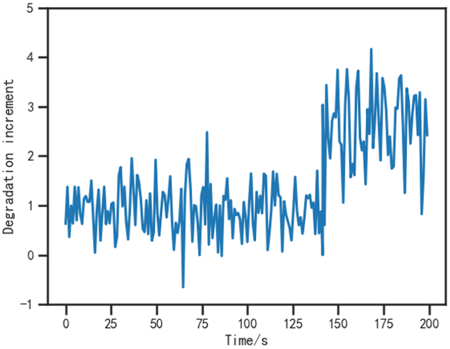
The degradation increment trajectory of sample 6.

Figure 8.

Prediction results of change points for sample 6 $[\tau =132\mathrm{s}]$ : (a) predicted mean and variance and (b) probability of change point.

To validate the superiority of the proposed change-point detection method, we conducted comparative experiments on the aforementioned 150 simulated sample groups using three different change-point detection methods: Method A (Bayesian approach), Method B (Pettitt’s non-parametric method), and Method C (CUSUM). Notably, Methods A and C were implemented with optimized parameters as specified in Table 2.

Table 2.

Change point detection results comparison.

Method	Initial parameters	[Maximum lead error, maximum lag error]Maximum error range	Improvement over B	Improvement over C
A: Bayesian	${\mu }_1=0.81,{\mu }_2=2.31,{\sigma }_1=0.42$ , ${\sigma }_2=0.78,\tau =148$ .2	[0, 6] 6	78.5%	85%
B: Pettitt	/	[28, 0] 28	/	/
C: CUSUM	warmup_period = 25, delta=20, threshold = 5	[−20, 20] 40	/	/

Figure 9 presents the accuracy comparison of the three methods. In terms of prediction error ranges, the proposed Bayesian change-point detection method (Method A) demonstrated the highest precision with errors confined between 0 and −6. The Pettitt method (Method B) showed errors ranging from 0 to 28, while the CUSUM method (Method C) exhibited fluctuating errors between −20 and 20. Quantitatively, the Bayesian method achieved approximately 78.5% and 85% accuracy improvements over the Pettitt and CUSUM methods, respectively. Furthermore, Figure 9 reveals that as change-points occur later in longer time series, both Pettitt and CUSUM methods tend to produce larger prediction errors.

Figure 9.

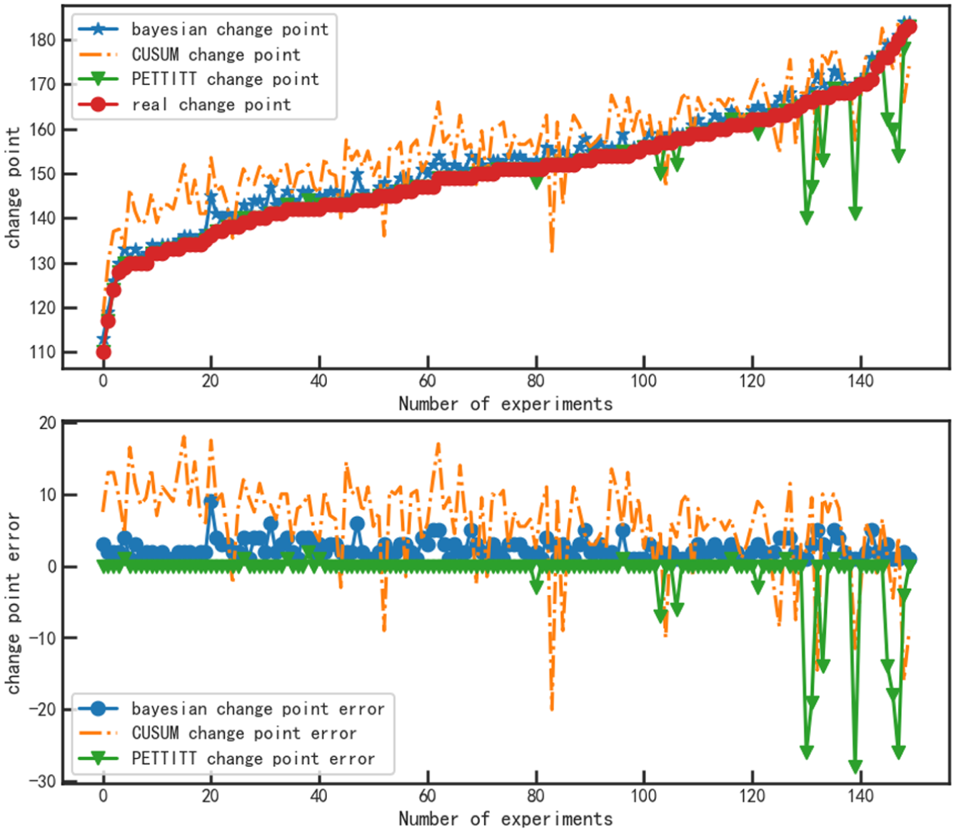
Error analysis of three change-point detection methods.

Figure 10 analyzes the impact of change-point prediction errors on remaining useful life (RUL) estimation. The results demonstrate that: (1) RUL prediction errors increase with larger change-point detection errors, and (2) negative change point prediction errors (indicating premature detection) lead to more significant RUL estimation inaccuracies.

Figure 10.

Impact of change point errors on RUL predictions.

Combining the analyses from Figure 9, we observe that the Bayesian method consistently produces smaller lagging errors in change-point detection. Compared to the Pettitt method, this characteristic enables the Bayesian-based approach to significantly enhance RUL prediction accuracy.

Figure 10 analyzes the impact of change point prediction errors on RUL predictions. When the change in predicted change point error ranges from −12 to 12, the figure shows:

• (1) The error in RUL predictions increases with the change point prediction error;

• (2) When the change point prediction error is negative (predicted change points ahead of actual change points), the error in life predictions is more significant. Combining the analysis of Figure 9, it can be concluded that the Bayesian change point detection method, due to its lagging errors and relatively small error values, helps improve the accuracy of RUL predictions compared to the Pettitt and CUSUM method.

For sample 6, the degradation threshold is $\omega =200$ . According to Algorithm 2, real-time updates of parameters are performed. Substituting into the remaining life PDF formula, the RUL prediction results at each moment and the PDF distribution are shown in Figures 11 and 12, respectively. From the results, after accurately predicting the change points, the RUL predictions achieved satisfactory results.

Figure 11.

RUL results of sample 6.

Figure 12.

RUL PDF of sample 6.

Case study

The sample data comes from the bearing dataset XJTU-SY, ²² which contains vibration signal data of 15 rolling bearings over their full life cycle under three different operating conditions. The test setup comprises an AC motor, a motor speed controller, a shaft, supporting bearings, a hydraulic loading system, and the test bearings. The model of the experimental bearing is LDK UER204 rolling bearing. In the test setup, the bearing vibration sampling frequency is $25.6\mathrm{kHz}$ , the sampling interval is 1 min, and the duration of each sample is 1.28 s.

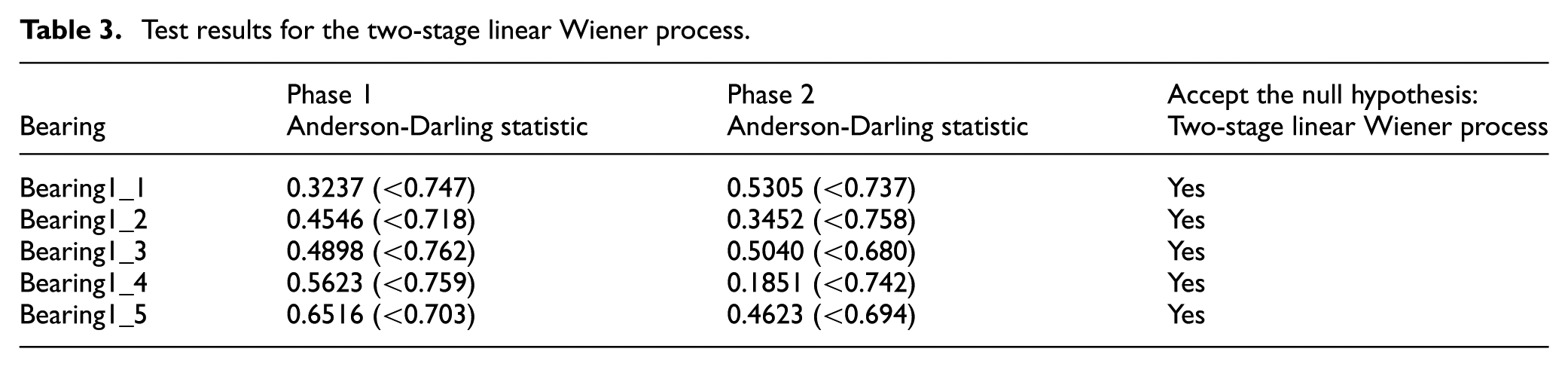
Five sets of full-lifecycle degradation data (Bearing1_1, Bearing1_2, Bearing1_3, Bearing1_4, and Bearing1_5) were selected from the degradation database. The kurtosis index was chosen as the degradation indicator. After defining a dimensionless maximum kurtosis value of 30, the indicator was normalized to a 0–1 scale. Data from the latter two stages of the bearing degradation lifecycle (i.e. the medium-term degradation and late-term degradation stages) were retained, and the resulting degradation curves are shown in Figure 13. Next, we examined whether the degradation data conform to the two-stage linear Wiener process model (as shown in equation (3)). The method for testing whether a process fits a linear Wiener process is as follows: first, difference the degradation curve, and then, at a significance level of 0.05, verify whether the differenced signal satisfies the normality assumption. Initially, the five sets of degradation curves were assumed to follow a single linear Wiener process. The Anderson-Darling (AD) test was applied to the entire set of five curves. The AD test statistics for the five datasets were [13.8657, 5.4448, 6.9816, 17.8811, 6.9216], all exceeding the 5% critical values [0.762, 0.765, 0.765, 0.742, 0.733]. This indicates that the curves do not conform to the assumption of a single linear Wiener process. Using any of the three aforementioned methods (Bayesian, Pettitt, or CUSUM), optimal change points were detected for the five datasets. Each curve was segmented into two phases based on the detected change point. The two segments (Phase 1 and Phase 2) were then separately tested for adherence to a linear Wiener process. The change point locations and AD test results are summarized in Table 3. The results show that after segmentation, the AD test statistics for both segments of each curve are lower than the 5% critical values, meaning the null hypothesis cannot be rejected. This confirms that both segments of the degradation curves after segmentation conform to a linear Wiener process.

Figure 13.

Degradation trend of rolling bearings (bearing1_1–bearing1_5).

Table 3.

Test results for the two-stage linear Wiener process.

Bearing	Phase 1Anderson-Darling statistic	Phase 2Anderson-Darling statistic	Accept the null hypothesis: Two-stage linear Wiener process
Bearing1_1	0.3237 (<0.747)	0.5305 (<0.737)	Yes
Bearing1_2	0.4546 (<0.718)	0.3452 (<0.758)	Yes
Bearing1_3	0.4898 (<0.762)	0.5040 (<0.680)	Yes
Bearing1_4	0.5623 (<0.759)	0.1851 (<0.742)	Yes
Bearing1_5	0.6516 (<0.703)	0.4623 (<0.694)	Yes

To validate the effectiveness of the proposed method, two state-of-the-art lifespan prediction approaches were selected for comparison. Method 1, proposed in Gebraeel et al., ¹⁰ employs a Bayesian updating approach based on a Brownian motion with error process to predict the remaining useful life distribution of equipment using real-time degradation signals. Method 2, introduced in Zhang et al., ¹⁹ is a multi-stage stochastic degradation modeling approach for lifespan prediction that utilizes CUSUM-based change point detection. The proposed Bayesian change point detection method in this paper is designated as Method 3. The model error is defined as the Maximum Absolute Error (MAE), which is the sum of the absolute values of multiple lifespan prediction errors.

For the comparative experiments involving the three methods, four sets of degradation bearing data (Bearing1_2, Bearing1_3, Bearing1_4, and Bearing1_5) were selected as offline data, with Bearing1_1 used as the online bearing. Based on the monitored data up to each time point (t _k ), the probability density function (PDF) of the remaining useful life (RUL) and the point estimate of the lifespan were predicted.

The degradation curve (excluding the early slow degradation data of the rolling bearing) is shown in Figure 13, and the failure threshold is set to 0.9.

In method 3, the prior parameters of the model were estimated to be: ${\mu }_1=0.003,{\mu }_2=0.034,{\sigma }_1=0.01,{\sigma }_2=0.05,\tau =75$ , according to the method in Section “Offline parameter estimation.” Using the offline estimated prior parameters as the hyperparameters for the Bayesian change point detection method, which are $m_0=0.003,v_0=10,a_0=5,B_0=0.0004$ , the differential curves and change point probability graphs are shown in Figure 14. Real-time change point prediction indicates that the change point location is 61. The corresponding remaining life prediction results and PDF distribution are shown in Figures 15 and 16, with fairly accurate remaining life predictions obtained at various prediction points throughout the entire life cycle.

Figure 14.

Bayesian change point detection result (bearing1_1): (a) predicted mean and variance and (b) probability of change point.

Figure 15.

RUL prediction results.

Figure 16.

RUL PDF of Method 1.

For the remaining useful life (RUL) prediction of Bearing1_1, a comparison of the results from the three methods is shown in Table 3, with visualizations provided in Figures 15 to 18. Analysis of the outcomes reveals that Method 1, based on a single-stage model, produces substantial errors in RUL prediction, with forecasts at certain time points reaching unacceptable levels. In contrast, both Method 2 and Method 3, which incorporate change point detection, generally achieve smaller prediction errors. However, the change point identified by the CUSUM-based Method 2 occurs at 68 (with an 8-point lag), resulting in overall larger prediction errors. As can be seen from Table 4, its MAE value is 907, whereas the MAE of the proposed method is 408, demonstrating the best prediction performance.

Figure 17.

RUL PDF of Method 2.

Figure 18.

RUL PDF of Method 3 (Proposed).

Table 4.

Prediction errors and comparison of the three methods.

Method	Method 1	Method 2	Method 3 (Proposed)
MAE	3625	907	408

Conclusion

In response to the multi-stage characteristics of random change points in the operational degradation process of rolling bearings, this paper proposes a novel multi-stage RUL prediction method based on Bayesian change point detection. Through analysis and experimental validation, the following conclusions are drawn:

• (1) The proposed life prediction method employs Bayesian change point detection, which improves the accuracy of change point detection by 85% compared to other methods, thereby enabling high-precision multi-stage RUL prediction.

• (2) his method is applicable throughout the entire lifecycle of bearing degradation, including both before and after the occurrence of change points. Particularly in the first stage (before the change point), it leverages prior estimates of change points and second-stage parameters derived from offline data to achieve relatively accurate RUL predictions.

• (3) The proposed method adopts online inference for prediction, where change points are detected by generating the precise distribution of the next unobserved data point given the observed sequence. This approach belongs to real-time online change point detection and, when combined with real-time parameter updating, can be applied to online RUL prediction.