Development of an innovative framework for the simulation of freight trains longitudinal dynamics

Abstract

This paper presents SIMTRAD or SIMulation of TRAin Dynamics, an innovative framework for simulating longitudinal dynamics of freight trains. The framework integrates detailed sub-models of locomotives, wagons, couplers, and adhesion dynamics inside a modular Simulink environment, thus enabling flexible and accurate simulation of train operations. In contrast to multibody software—which mainly address the overall dynamic behaviour of railway vehicles—SIMTRAD is tailored to capture the longitudinal interactions within the train. SIMTRAD enables detailed modelling of locomotives, wagons, braking systems, and couplers, offering broad and flexible application possibilities. The proposed methodology has been validated against established software, demonstrating consistency in predicting longitudinal compressive and tensile forces acting on train couplers. A case study has also been then conducted, with the aim to optimize freight train composition by minimizing in-train forces through the optimal placement of locomotives and payload distribution. The results highlighted reductions of 53% in the values of Longitudinal Tensile Forces (LTFs) and of 7% for the Longitudinal Compression Forces (LCFs), contributing to enhanced train performance and operational efficiency. This framework also supports future integration with Hardware-in-the-Loop systems, broadening its application to different scenarios across academic research and the industrial domain related to the railway sector.

Introduction

Railway transportation is pivotal to enhancing the environmental and logistical efficiency of Europe’s freight sector, offering a sustainable solution to reduce the carbon footprint while increasing the volume of goods transported. To fully harness these benefits, better utilization of existing infrastructure is essential, which has led to a push for accommodating longer and heavier freight trains. Currently, European railways are designed for trains up to 750 m in length, but discussions are underway regarding the possibility to upgrade key corridors to allow convoys of up to 1500 m, thus aligning infrastructure capabilities with the growing demand for more efficient and sustainable logistics. ¹

Heavier trains often require the presence of a second or third locomotive to deliver the required tractive effort. The placement of additional locomotives is not a straightforward task, since it influences the tensile and compressive forces acting on the whole length of the trainset and can, in certain limit scenarios, even cause couplers to fail or vehicles to derail. ² Moreover, longer trains may pose higher stresses on their drivers, thus requiring additional training and technological aid. ³ Finally, additional requirements related to other aspects of rail transportation (such as terminal operations, train assembly and disassembly, etc.) can impose further constraints on the optimal placement of additional locomotives within the trainset. ⁴

A set of optimal solutions for the placement of the additional locomotives can be obtained using longitudinal simulation of train dynamics. ⁵ These tools allow to predict the maximum compressive and tensile forces developed by the couplers during operations. An example of the application of this procedure can be found in Krishna et al. ⁶ : here, statistically significant populations of freight trains are tested during braking maneuvers, finding that that the best position for a second locomotive to minimize longitudinal compressive and tensile forces is roughly at two thirds of the trainsets.

Such an optimization procedure can be extended to the payload distribution along the whole trainset: being the arrangement of vehicles one of the operational parameters which can greatly influence the forces exchanged along the couplers during trainset maneuvers, ⁷ an optimal distribution of laden and empty wagons along the train can significantly affect both Longitudinal Compressive and Tensile Forces. An investigation regarding the effects of payload and locomotive placement on in-train forces has also been performed by Di Gialleonardo et al. ⁸ and Mazzeo et al. ⁹ : a statistically significant set of trains, each having a different payload distribution, is generated and the order of vehicles or position of locomotives is optimized with the aim of minimizing longitudinal forces during a brake application manoeuvre. Moreover, Arcidiacono et al. ¹⁰ has developed a statistical to optimize payload distribution in freight trains, significantly reducing the number of simulations required to analyze critical longitudinal forces (compression and tension) during maneuvers, ensuring improved safety and operational efficiency.

Several software for longitudinal train dynamics analysis have been developed.^11,12 Unlike established multibody software tools such as GENSYS, VAMPIRE, and SIMPACK—which primarily focus on the comprehensive dynamic behavior of railway vehicles—these are primarily dedicated to capturing the forces that are exchanged within the entire trainset as consequences or different maneuvers. A notable mention is represented by the approach highlighted in Pugi et al., ¹³ where a library of several sub-models of a UIC freight braking system is developed and validated against experimental data. A similar modeling approach was thus selected for this work.

Finally, the introduction of the Digital Auto Coupler or DAC has the potential to radically streamline the process of freight trains composition, diagnostic and operations. The addiction of Electro-Pneumatic braking and the possibility to enable a continuous verification of train integrity has the potential of becoming a disruptive technology in the railway field. However, the introduction of a new coupler into the European railway fleet requires studying the mechanical dynamics and behavior differences compared to traditional couplings, especially in the crucial transitional period. ¹⁴ To properly model the new features of the DAC, such as the possibility of EP braking or its possible interaction with other train components, a more flexible suite is thus needed.

This work aims to contribute to the field of longitudinal dynamics of freight trains by achieving two main objectives. First, it introduces SIMTRAD or SIMulation of TRAin Dynamics, an innovative methodology for simulating the longitudinal dynamics of freight trainsets, detailing its key features and validating its accuracy against an established train dynamics software. It then applies the proposed framework with the aim to optimize freight train composition, focusing on both locomotive placement and payload distribution, with the goal of minimizing in-train forces and enhancing operational efficiency. Some final conclusions on the obtained are then drawn.

Methodology

The methodology used for this work is based on the simulation of longitudinal dynamic of a freight train via a Simulink toolbox. Its focus is similar to that of TSDYN (Train-Set DYNamics simulator), a detailed model developed by the Department of Mechanical Engineering of Politecnico di Milano to study longitudinal dynamics of freight trains.^15,16 However, SIMTRAD distinguishes itself by offering a higher level of detail in the modeling of the inner functioning of key train components, such as wagons, locomotives, braking systems, and couplers.

Simulink is chosen as it simplifies the visual representation of system components and their interactions through its user-friendly graphical interface. Moreover, it allows the assembly of a trainset so that each subsystem can be directly correlated with the physical component it models.

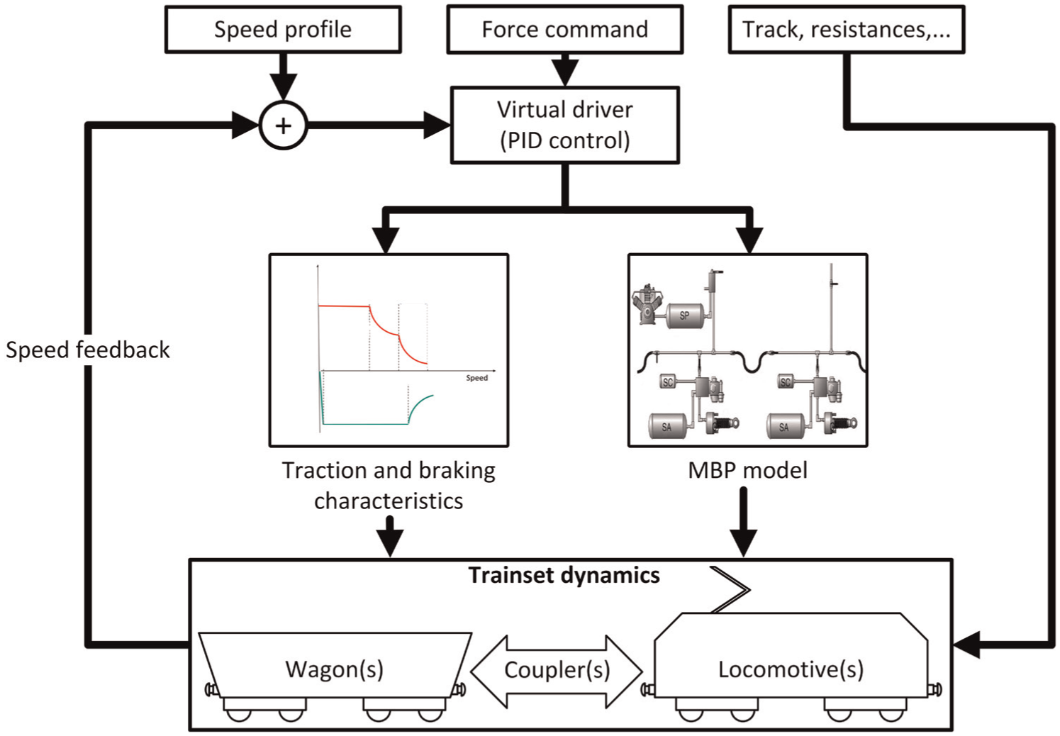
The main objectives of the simulation are to model the braking and traction systems, the connection between wagons as well as the exchange of traction and braking forces. The wheel-rail interaction and the adherence are also introduced. A general representation of the model layout is given in Figure 1. The assembly process followed in this work, as well as a description of the main components, is given in the following paragraphs.

Figure 1.

General architecture of the Simulink model

The toolbox comprehends a main Simulation environment as well as a library of Submodels, each representing a specific component (a locomotive model, a wagon, a coupler) or a subcomponent (the adhesion model, a specific type of brake regulator). Finally, a set of routines allow the assembly of a functioning trainset starting from the said library and the analysis of the simulation results.

The toolbox and the models are designed to have modularity and compatibility as key requirements. This approach facilitates iteration and optimization of the model, enabling more efficient design and better understanding of system dynamics.

Additionally, the toolbox architecture enables the integration of subsystems developed by independent entities, including models whose internal characteristics are proprietary or protected for industrial confidentiality, by incorporating them as black-box components. Finally, it allows the future implementation of Hardware in the Loop or HiL components within the simulation environment. This feature broadens the application range of this methodology and allows for more precise results by accurately replicating the authentic behavior of specific components.

Self-assembly model

The creation and assembly of the various sub-models which compose the trainset model are performed by means of automatic programming through MATLAB scripts. This aims at providing enhanced flexibility, control, and reproducibility, as well as an easy reconfiguration of the sub-models when assembling trainset with different characteristics. Moreover, this approach facilitates iteration and optimization of the model.

All the relevant data related to the simulation is stored in a single input file, which is processed by means of a set of MATLAB routines to automatically assemble the trainset starting from the sub-components library within the framework. The approach of using a single input file offers numerous advantages in terms of flexibility and ease of model customization. Users can easily modify system parameters and configurations by simply updating the input file, without the need to make direct changes to the Simulink model. This greatly simplifies the process of adapting the system to specific requirements or variations. All the relevant data then is passed down to the sub-models by means of a struct type data structure, which contains all the information related to the trainset composition, placement, and type of each vehicle within the convoy. This structure also includes essential data such as mass, inertia, geometry, suspensions which characterize each sub-component, as well as data regarding track’s geometry.

Suite components

The following paragraphs describe the main suite models implemented within the proposed suite.

Couplers

The force generated by the coupler is computed as the sum of the forces developed by the two buffers and the central hook. The hook is composed by an elastomer which can be modelled with a nonlinear spring in parallel with a nonlinear damper. If the distance between two adjacent wagons is such that it counterbalances the pre-tension of the coupling, the force exerted by the coupling itself is nullified.

The model used for the two buffers is based on the work and data collected by Cheli and Melzi ¹⁷ represented in Figure 2 and Figure 3: here, the buffer is modelled as the sum of the following contributions:

$$\begin{array}{c}{F}_b=F_p+F_s+F_{m,1}+F_{m,2}+F_f\hfill \end{array}$$

(1)

In this equation, the term F_s represents the contribution of the buffer’s linear spring, the two terms F_m,1 and F_m,2 consider the effects of two Maxwell elements, the term F_p represents the buffer’s preload and the term F_f represents the contribution of the internal buffer friction if the coupler is subjected to a misaligned load. This model allows to better reproduce the buffer’s dynamic behavior. Finally, the effects of preload or slack can also be added to the couplers.

Figure 2.

Forces exchanged along each coupler

Figure 3.

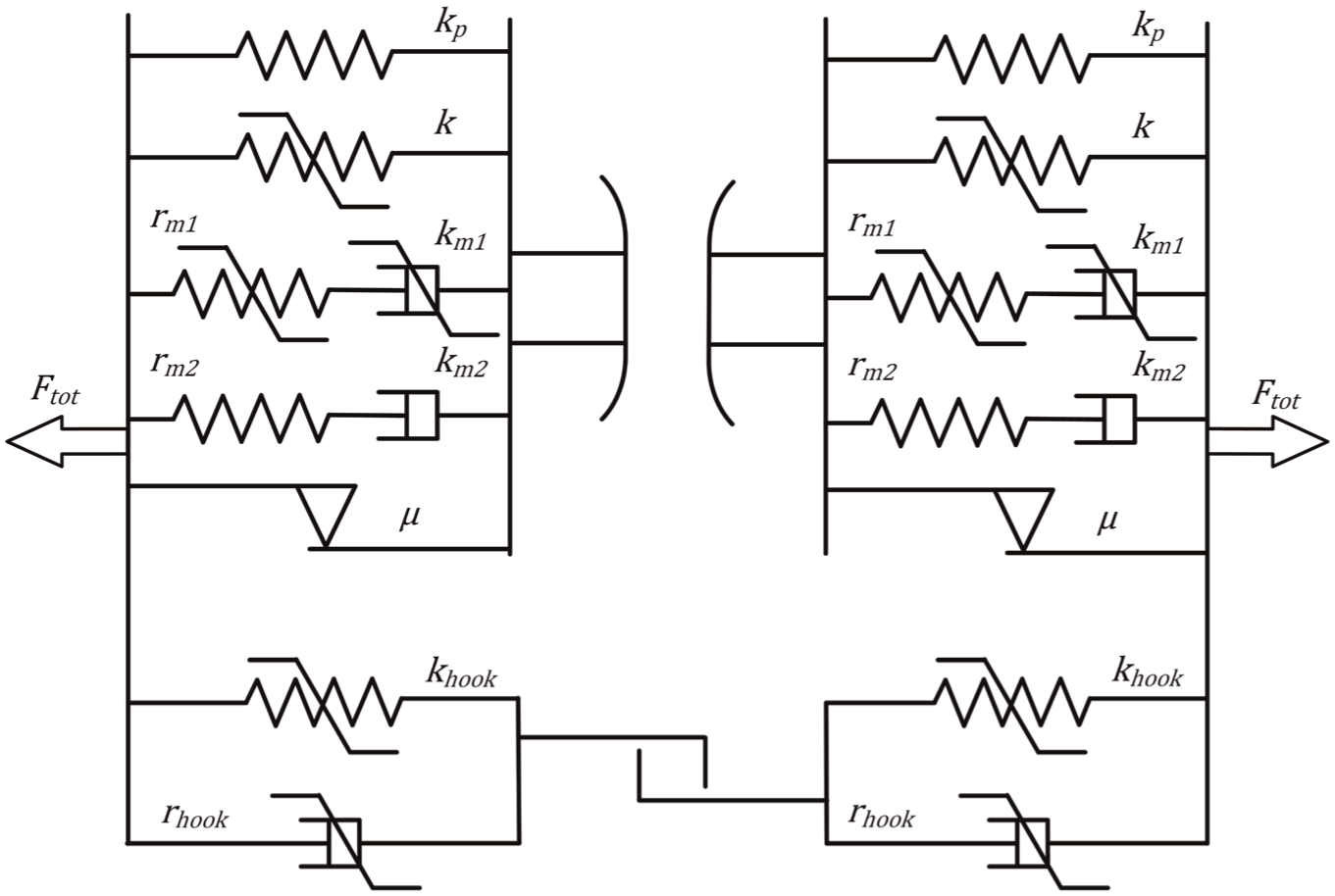
Complete coupler model used in the Simulink suite

Locomotive and adhesion

The locomotive submodel receives the mission profile and the forces acting on its buffers as inputs. Traction and braking commands, as well as the maximum velocity target, are the input to each locomotive during the simulation. From the mission profile and the current position and velocity of the locomotive, a virtual driver model based on a PID control regulates the traction or braking requests in order to respect the imposed input. In case of remote control of a second (or third) slave locomotive physically disconnected from the trainset head, a delay in the control loop is introduced to take into account the time required by the wireless control logic of the slave locomotives more realistically. ⁶

A generalized architecture of the forces acting on the locomotive is given in Figure 4, while the speed control model, used to evaluate the traction and braking forces of the total vehicle is showed in Figure 5.

Figure 4.

Longitudinal forces acting on each locomotive

Figure 5.

Locomotive speed control architecture

The traction creep forces are computed for each wheelset independently using the Polach tangential model. ¹⁸ More in detail, starting from the vertical load on each wheelset (in the 1D model the vertical load on each wheelset is calculated starting from the total locomotive mass which is then distributed over the four wheelset equally as in static conditions, although the model retains the possibility of modelling load redistribution on locomotive axles) it is possible to use the Hertz Theory ¹⁹ to evaluate the size of the contact patch semi-axis as function of the wheel, rail material and geometrical characteristics.

At the current stage of the modelling process, starting from the output of the Hertz model and the angular and longitudinal velocities of each wheelset, it is possible to evaluate the creep forces on each wheel-rail contact patch as function of the tangential stress gradient, according to Polach theory, as shown in equation (2).

$$\begin{array}{c}F=-\frac{2\mathrm{Qf}}{\pi }(\frac{\epsilon }{1+{\epsilon }^2}+{\tan }^{-1}\epsilon )\hfill \end{array}$$

(2)

where $Q$ is the vertical load, $f$ is the friction coefficient and $\epsilon$ is the gradient of the tangential stress in the area of adhesion and it has been calculated as follow:

$$\begin{array}{c}\epsilon =\frac{2}{3}\frac{C\pi a^{2}b}{\mathrm{Qf}}·s\hfill \end{array}$$

(3)

with $a$ and $b$ that represent the semi-axis of the contact patch, s which is the creep and $C$ which represents the proportionality coefficient characterizing the contact elasticity. ¹⁸

Furthermore, traction and braking efforts are exchanged between vehicle and track at the wheel/rail interface, and it is fundamental to consider the available adherence, which depends on different parameters, such as the vehicle speed. From the other side, starting from the real traction curve of each electric motor it is possible to evaluate the traction torque applied on the wheelset axle and then by also knowing the creep force it is possible to evaluate the angular acceleration and velocity (by means of the time integration block in Simulink) of each wheelset.

The longitudinal dynamic equilibrium of the resistance, traction, braking and coupling forces are then used to compute the total forces acting on the locomotive, which can be in turn divided by the equivalent mass (that is the equivalent inertial mass and also includes the contribution of rotating masses as wheelsets, motors and transmission systems) to obtain its instantaneous acceleration. Finally, by using time integration Simulink blocks it is even possible to evaluate the longitudinal velocity and the position along the prescribed track of the vehicle. The updated position of the locomotive, as well as the position of the adjacent wagons, is finally used to compute the forces acting on its couplers at the next integration step.

Wagons

From the point of view of the wagons sub-model architecture, each wagon characteristics are listed in the input file. Furthermore, each wagon sub-model, based on its position along the input track and velocity, can compute all the resistance values (gradient resistance, curve resistance, aerodynamic and friction losses, …). Appropriated formulas for these values are computed according to Iwnicki. ²⁰

The dynamic equilibrium of the resistance, braking and coupling forces are then used to compute the total forces acting on the vehicle, which can be in turn divided by the mass to obtain its instantaneous acceleration and hence its subsequent speed and position. A reference diagram of all the forces acting on each wagon is depicted in Figure 6.

Figure 6.

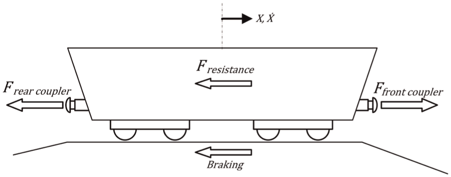
Longitudinal forces acting on each wagon

The payload carried by each wagon can be adjusted based on the input file: it contains a vector containing percentages of the maximum payload capacity of the whole train. Each wagon block then computes its own total adhesive mass, which is used for all dynamic computations. This approach allows to deal with simulations involving several identical vehicles with different payloads, a typical situation in railway operations.

At the current stage of the modelling process, a relatively simplified braking system has been implemented in each wagon model. At first, the dynamics of the braking pipe is solved off-line on a separate code based on the equations detailed in Melzi and Grasso. ¹⁵ The time series of the brake cylinders’ pressures is then used to compute the braking force on each vehicle.

Possibility of combining the methodology with HiL devices

A Hardware-in-the-Loop (HiL) system enables real-time simulation by integrating physical hardware components with a virtual model, providing a robust platform for testing and validation. These platforms have been successfully employed in a number of different fields, ranging from the study of catenary-pantograph interaction, pneumatic air brakes and traction equipment.^21–24 The Simulink suite described in this work is capable of interfacing seamlessly with various Real-Time Target machines (such as Speedgoat P3) which in turn can communicate with HiL test benches via both EtherCAT or analog inputs/outputs, allowing for the simulation of multiple aspects of a freight train, such as braking systems, connectors, and other critical subsystems. These goals are achieved through fixed-time step integration, the use of closed-form equations and the possibility to simplify the non-necessary submodels to ease the computation load on RTT machines.

Model validation

The proposed methodology is validated via a comparison with the software TSDYN (Train-Set DYNamics simulator), a detailed model developed by the Department of Mechanical Engineering of Politecnico di Milano to study longitudinal dynamics of freight trains. A detailed overview of TSDYN is given in Melzi and Grasso ¹⁵ and Belforte et al. ¹⁶

To accomplish this, a set of 1000 trainset having different characteristics is generated. Each trainset is composed by three E402B locomotives (commonly employed in Italian railways for freight transport) and several SGMNSS railcar, each of them having a random payload so that the trainset reaches either the maximum allowed mass (3200 t) or the maximum allowed length (1500 m). Data regarding the two vehicles is summarized in Tables 1 and 2. Two locomotives are placed at the head of the trainset, while the third one is placed at the back. This dataset can therefore be assumed as a statistical representation of the possible spectrum of trainsets which might be allowed to circulate on European railways. The following tables recall the main parameters of both locomotives and SGMNSS cars.

Table 1.

Principal characteristics of the E402B locomotive.

Variable	Value	Unit of measurement
Mass	88,080	kg
Length	19.42	m
Maximum speed	220	km/h
Maximum traction effort	265	kN

Table 2.

Principal characteristics of the SGMNSS wagon.

Variable	Value	Unit of measurement
Maximum payload	73,500	kg
Tare mass	16,500	kg
Length	17.25	m

For each member of the population, the Simulink model of the trainset is generated and is commanded to start from a standstill with an acceleration of 0.1 m/s² for a time of 60 s on straight track. This first scenario in chosen to validate the framework’s ability to investigate scenarios where extremely high coupler forces are imposed by locomotives during starting.

Subsequently, the Simulink model is commanded to execute an emergency braking maneuver from a velocity of 30 km/h up to the complete arrest of the trainset. The second scenario is chosen to validate the framework’s ability to investigate the behavior of couplers during large deceleration typical of emergency braking.

After each simulation, the maximum tensile and compressive force acting on the whole trainset are recorded. Each member of the population is also analyzed through TSDYN and asked to perform the same maneuver.

The analysis is extended to the whole population: for each trainset, the maximum longitudinal forces computed via Simulink and TSDYN during the simulation are computed. In Figure 7, each circle represents the values obtained via Simulink (on the Y axis) and on TSDYN (on the X axis), during both maneuvers (start from a standstill and emergency braking).

It is possible to appreciate how maximum LTFs and LCFs computed during acceleration are highly clustered together and close to the maximum (or a multiple of the) traction effort of a single locomotive. This can be explained by the fact that the maximum compressive or tensile force is exercised on the coupler closest to one of the locomotives. On the contrary, LTFs computed during braking are close to zero and LCFs exhibit a larger dispersion, both in terms of values and differences among the two methodologies. This can be explained from the different modelling of the buffers: TSDYN uses a simpler coupler model, neglecting any velocity-varying stiffness and damping.

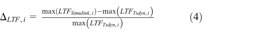
In order to better quantify the error between the Simulink and TSDYN results, the average non-dimensional difference of both LFCs and LTFs are computed as:

$$\begin{array}{c}{\mathrm{\Delta }}_{\mathrm{LTF},i}=\frac{max\left(\mathrm{LT}{F}_{\mathrm{Simulink},i}\right)-max\left(\mathrm{LT}{F}_{\mathrm{Tsdyn},i}\right)}{max\left(\mathrm{LT}{F}_{\mathrm{Tsdyn},i}\right)}\hfill \end{array}$$

(4)

$$\begin{array}{c}{\mathrm{\Delta }}_{\mathrm{LCF},i}=\frac{max\left(\mathrm{LC}{F}_{\mathrm{Simulink},i}\right)-max\left(\mathrm{LC}{F}_{\mathrm{Tsdyn},i}\right)}{max\left(\mathrm{LC}{F}_{\mathrm{Tsdyn},i}\right)}\hfill \end{array}$$

(5)

Figure 7.

Maximum LTF and LCF obtained on the same trainset performing the same manoeuvre both on Simulink (y axis) and on TSDYN (x axis)

Figure 8 depicts both the mean and the standard deviation of the error between the two methodologies computed across the whole population for both LTFs and LCFs using the boxplot analysis: the median of the population is represented with the red lines, the 25-th and 75-th percentile are represented by the lower and upper base of the rectangles and the extreme values of the distributions are indicated by the horizontal lines at the top and the bottom of each plot (called whiskers).

Figure 8.

Mean and standard deviation of the error on between the LTF and LCF computed on both Simulink and TSDYN

The error computed during the acceleration scenario shows remarkably low values (Mean absolute error of 0.2% and root mean square error of 0.8% for LTFs, MAE of—1.23% and RMSE of 0.7% for LCFs), while errors became slightly larger—but still acceptable—for braking manoeuvres (MAE of 3.8%, RMSE of 11.3% for LCFs and MAE of 11.2% and RMSE of 11.1% for LTFs). While the larger error seen in LCFs for braking manoeuvres can be explained by the different model used for couplers, a simpler reason causes an increase in the LTF error: during the braking manoeuvre, hooks are subjected to very small forces: Figure 7 confirms this hypothesis. Thus, even minor differences of traction forces can create, in relative terms, large absolute errors.

The overall performance of the methodology is deemed satisfactory, and the optimization procedure can thus be performed.

Case study: Payload and locomotive position in a freight trainset

The following chapter presents a detailed examination of the optimization process, utilizing the Simulink suite as the primary computational tool.

Statement of the optimization procedure

When dealing with optimization problem, the most reliable and common approach would be the evaluation of the objective function on all the possible combinations within the search space. However, this approach becomes impractical when the search space is large due to the significant computational cost. Therefore, employing an optimization algorithm that accelerates the search process and delivers high-quality solutions (even if not guaranteed to be optimal) within a reasonable timeframe is a more practical approach. Meta-heuristic algorithms have been designed to address such optimization problems, particularly when conventional methods prove less effective or efficient. Among all the possible meta-heuristic algorithms, the methodology presented and validated in Alazzam and Iii ²⁵ is chosen as the optimization strategy, since it allows for a general-purpose stochastic search method based on derivative-free simulations similar to other evolutionary algorithms like, for example, genetic algorithm (GA). ²⁶ A representation of the operating procedure of the chose algorithm can be appreciated in Figure 9.

Figure 9.

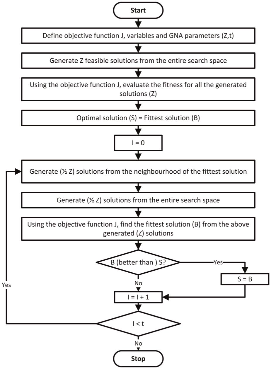
Scheme of the GNA algorithm used in the optimization procedure

Two different objective functions were defined to evaluate the fitness of each given train: the first objective function J₁ aims at representing the effect of the sole Longitudinal Tensile Forces

$$\begin{array}{c}{J}_1=max\left(\mathrm{LT}{F}_{i,j}\right)\hfill \end{array}$$

(6)

This fitness function neglects the effects of the compressive forces acting on the trainset. These forces can be critical to assess the derailment risk of a convoy. Thus, a second fitness function is also used, which takes into account both LTFs and LCFs as done in Di Gialleonardo et al. ⁸ :

$$\begin{array}{c}{J}_2=\sqrt{max{\left(\mathrm{LT}{F}_{i,j}\right)}^2+\max {\left(\mathrm{LC}{F}_{i,j}\right)}^2}\hfill \end{array}$$

(7)

Each of the two trainsets population is therefore optimized according to both J₁ and J₂.

The optimization process for arranging a train with n vehicles (where the leading locomotive’s position is fixed at the head of the train) is based on the following procedure. At first, a population of Z vehicle is randomly generated. Z is set at:

$$\begin{array}{c}Z=2\mathrm{floor}\left(\frac{n-1}{2}\right)\hfill \end{array}$$

(8)

A set of Z convoys is therefore generated, the maneuver is simulated, and the fitness J is computed based on the coupling forces. Two offspring sets of Z/2 elements each are then generated: one randomly selected from the global search space, and the other derived by modifying the positions of two wagons near the best-known solution. For each of the elements of this new set, the fitness is computed and evaluated as before. The process repeats until one of the stopping criteria is met: either the improvement in fitness is below a threshold of 0.01% (indicating convergence) or the maximum number of iterations (100) is reached.

Results

For the optimization problem, two populations of 1000 trains each are considered. Each train consists of three E402B locomotives, commonly used in Italian railways for freight transport, and a variable number of SGMNSS railcars. The payload of each railcar is randomized such that the trainset reaches either the maximum permitted mass of 3200 tons or the maximum allowable length of 1500 m.

Both populations are constructed with a homogeneous mass distribution along the trainset length. The first set will be optimized by freely moving all the locomotives and wagons along the trainset, to reduce the forces exchanged between wagons. The second set undergoes the same optimization procedure, with the additional constrain of the third locomotive to be fixed at the end of the trainset. This additional constraint is intended to reflect the operational limitations of train services, where payload capacity and trainset composition must be balanced against the practicality of assembly and configuration.

During the optimization, the average number of iterations required to reach convergence among all the population was 26, with a standard deviation of 15 iterations.

Population 1: LTF minimization

Figure 10 shows the optimized mass distribution of the first train population when only the Longitudinal Tensile Forces are targeted for optimization. It is possible to appreciate how the resulting mass distribution results in loaded wagons being immediately behind each locomotive, while the empty wagons collect themselves in the first quarter of the trainset, halfway between the first and second locomotive. The third locomotive is placed at roughly 90% of the trainset length.

Figure 10.

Original trainset and optimal composition when minimizing only LTFs, no constrain in pushing locomotive

When looking at the maximum LTF and LCF data of both the original and optimized composition detailed in Figure 11, a strong decrease in Tensile Forces (which are now a fraction of the minimum breaking load of the screw-coupling as given by the standard EN 1566:2022) ²⁷ is accompanied by a sharp dispersion of Longitudinal Compression Forces.

Figure 11.

Maximum LTFs and LCFs in both original and optimized population when minimizing only LTFs, no constrain in pushing locomotive

Population 1: LTF and LCF minimization

The same train population is then optimized using equation (7) as the fitness function, thus aiming at the reduction of both LTFs and LCFs. The optimized payload distribution depicted in Figure 12 now exhibits three distinct “humps”, in the middle and near the extremities of the train. This is also where the two slave locomotives have been moved: each locomotive push and pulls the heaviest cars now in their proximity, while the empty wagons are clustered near the first and third quarter of the train.

Figure 12.

Original trainset and optimal composition when minimizing both LTFs and LCFs, no constrain in pushing locomotive

While Figure 13 shows the same decrease of LTFs encountered in the first optimization, the additional contribution of LCFs in the fitness computation allows for a significant decrease in both the magnitude and dispersion of LCFs. This improvement substantially reduces the overall stress experienced by the train population.

Figure 13.

Maximum LTFs and LCFs in both original and optimized population when minimizing both LTFs and LCFs, no constrain in pushing locomotive

In order to better understand the evolution of the coupler forces before and after the optimization procedure, the time histories of both LCFs and LTFs of one of the members of the population are extracted and represented in Figure 14. In this trainset, the new position of the second and third locomotive is set at 41% and 79% of the trainset respectively.

Figure 14.

Time histories of both LTFs and LCFs for the same trainset, before and after the optimization procedure

It is possible to appreciate how the new position of the locomotives along the trainset, as well as the payload redistribution, greatly influence the behavior of coupler forces over time. Both LTFs and LCFs are now distributed more evenly along the trainset and magnitude of their oscillation has declined.

Population 2: LTF minimization

Unfortunately, the complex arrangements required for the interposition of two locomotives within a freight trainset make the results of the first optimization round difficult to apply to real world application. The additional constraint of placing the third locomotive at the back of each train makes eventual trainset splitting and the insertion of the middle locomotive easier, since it can be accomplished with a single maneuver.

The additional constraint does not change the overall distribution of mass and the position of locomotives, as shown in Figure 15. However, Figure 16 highlights a decrease in the variability of the LCFs accompanied with a slight increase in its magnitude up to 260 kN.

Figure 15.

Original trainset and optimal composition when minimizing only LTFs, pushing locomotive kept at the train back

Figure 16.

Maximum LTFs and LCFs in both original and optimized population when minimizing only LTFs, pushing locomotive kept at the train back

Population 2: LTF and LCF minimization

Figure 17 depicts the results of the optimized mass distribution and locomotive placement of the second trainset population, with the additional constraints of the third locomotive being placed at the back of the train. In this configuration, the central cluster of heavily loaded wagons is broader, with the second locomotive situated near its leading edge. Similarly, the final cluster of heavy wagons is positioned directly in front of the rear locomotive.

Figure 17.

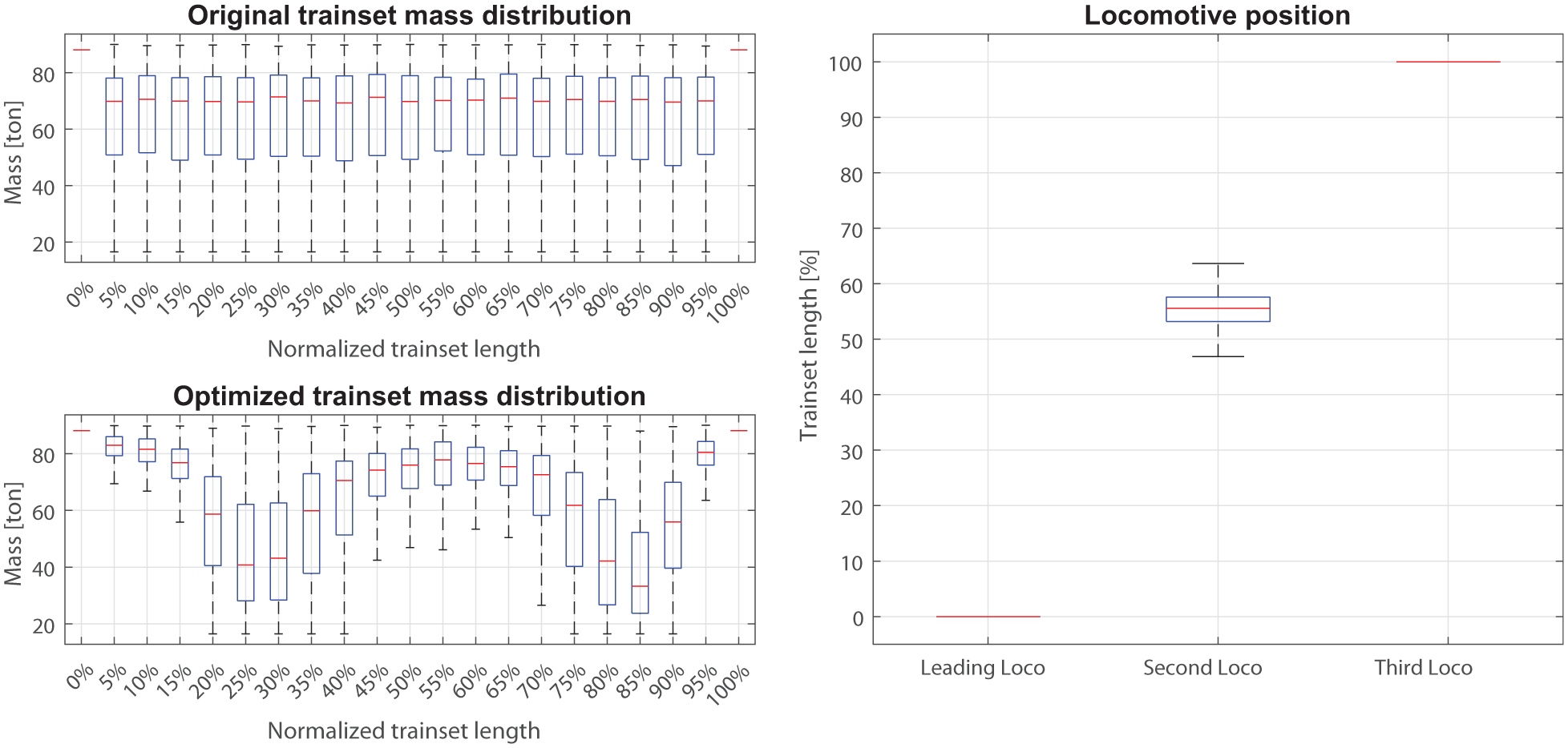
Original trainset and optimal composition when minimizing both LTFs and LCFs, pushing locomotive kept at the train back

From an operational perspective, this arrangement can be interpreted as the combination of three separate trains, each assembled independently and subsequently joined at a designated shunting yard to form a single, extended trainset for the remainder of the journey.

The magnitude of LCFs obtained with this analysis (and depicted in Figure 18) is slightly higher than the corresponding forces obtained without the third locomotive constrain. However, the total LTFs are drastically reduced and there is only a minor increase in the variability of LCFs.

Figure 18.

Maximum LTFs and LCFs in both original and optimized population when minimizing both LTFs and LCFs, pushing locomotive kept at the train back

All reductions in traction forces reported in the results are statistically significant, as confirmed by t-tests performed on the trainset populations before and after the composition optimization (maximum p-value = 1e−23; α = 1%).

Conclusions

This study introduces SIMTRAD or SIMulation of TRAin Dynamics, a novel simulation framework for analyzing the longitudinal dynamics of freight trains, leveraging a modular and customizable Simulink-based toolbox. The framework is validated against an established simulation suite, demonstrating accuracy in predicting longitudinal tensile and compressive forces during an acceleration maneuver. After validation, SIMTRAD is applied with the aim to find the optimal load distribution and locomotive placement of a population of overlong freight trains, obtaining solutions when targeting the optimization of longitudinal tensile forces only and of both tensile and compressive forces acting along the trainset. The composition of a second population is then performed, with the additional constraint of a fixed third locomotive at the end of each trainset. The results of the two optimization procedures show average reductions of 53% in the values of Longitudinal Tensile Forces (LTFs) and of 7% for the Longitudinal Compression Forces (LCFs) between the original and the optimized train population, thus enhancing safety. While the optimized solutions may in some cases require a redistribution of payload that does not always fully exploit the maximum capacity of every wagon, they provide a quantitative foundation for evaluating the trade-offs between payload maximization and the reduction of mechanical stresses on couplers and other critical components. Such trade-offs, although involving certain operational compromises, can yield benefits in terms of enhanced safety, reduced maintenance costs, and greater reliability.