Integrating experimental and mathematical approaches for AI-driven health monitoring of surface grinding machine

Abstract

High-precision surface finishing in manufacturing relies heavily on the condition of the grinding wheel, where any imbalance, cracks, or wear can degrade quality. This research aims to develop an AI-driven health monitoring framework by integrating experimentally acquired vibration data with a validated mathematical model, enabling accurate detection of grinding wheel conditions in real time. The study introduces a dual-framework approach combining statistical feature extraction from vibration signals with a physics-based model rooted in Newtonian mechanics and Fourier analysis. This integration enhances both the interpretability and robustness of fault classification, providing a novel, data-validated solution for predictive maintenance. Vibration signals were recorded for four wheel states—good, unbalanced, cracked, and worn—under controlled operational conditions. Ten statistically significant features, ranked using a Random Tree algorithm, were classified using a Random Forest model. Parallelly, a dynamic response model of the grinding wheel was developed and validated against experimental results. The Random Forest classifier achieved a 98.5% overall accuracy (Kappa = 0.98) using the top 10 features, with minimal misclassification (1.5%, primarily between cracked and unbalanced wheels). Mean vibration amplitudes ranged from 0.014g (good condition) to 0.078g (unbalanced), with one-way ANOVA confirming significant differences (p < 0.001). The mathematical model reproduced experimental accuracy trends, with classification performance stabilizing at 98.5% when ≥9 features were used, and maintained 96.8% accuracy under ±5% Gaussian noise. The proposed integrated approach enables high-fidelity, real-time condition monitoring of grinding wheels, reducing downtime and enhancing reliability. By coupling experimental validation with a physically grounded model and quantitative AI-based classification, this work surpasses conventional black-box approaches, offering an interpretable and industrially scalable predictive maintenance solution.

Introduction

In modern manufacturing, precision in surface finishing is paramount for producing high-quality machined components. ¹ Among various machining processes, surface grinding holds a crucial position due to its ability to deliver superior dimensional accuracy and surface finish.^2,3 This performance largely depends on the efficiency and condition of the grinding wheel. Any deterioration—such as wear, imbalance, or damage—can compromise the process outcome, leading to increased surface roughness, dimensional inaccuracies, and elevated rejection rates. Consequently, the grinding wheel’s efficiency significantly influences not just the surface quality but also the overall productivity and cost-effectiveness of the manufacturing operation.^4,5 Hence, the need for real-time health monitoring systems for grinding machines is more critical than ever.^4,6

The current investigation focuses on integrating experimental findings with mathematical modeling to develop an AI-based system capable of monitoring the health of surface grinding machines (Figure 1). The aim is to predict faults early by analyzing vibration signals and other physical phenomena associated with grinding wheel performance.

Figure 1.

Flowchart for AI-driven health monitoring integrating mathematical and experimental approaches.

Problem definition

Surface grinding is a highly sensitive process where wheel wear, imbalance, or damage can degrade the machining outcome.^7–9 Surface grinding is widely recognized for its ability to produce superior dimensional accuracy and excellent surface finish, especially when compared to conventional machining operations such as turning and milling. This capability stems from the fine abrasive interaction between the grinding wheel and the workpiece, which allows for minimal material removal with tight tolerances. As noted by Malkin and Guo, ¹⁰ grinding processes are capable of achieving surface roughness values in the nanometer range, making them ideal for precision finishing in industries such as aerospace, toolmaking, and automotive. Additionally, surface grinding offers improved geometrical control and consistency across batches, further supporting its role in high-precision manufacturing applications.^11,12

Recent studies have further highlighted the growing integration of machine learning and sustainability in grinding operations. For example, hybrid approaches have been proposed for optimizing minimum quantity lubrication (MQL) grinding conditions of Inconel 625, demonstrating the strong predictive power of machine learning techniques in modeling and process optimization. ¹³ Likewise, comprehensive reviews of the grinding process emphasize both technological advancements and challenges, including sustainability, hybrid cooling, and the increasing role of AI in fault detection and process optimization. ¹⁴ In parallel, environmentally benign grinding studies have shown the benefits of combining machine learning with eco-friendly lubrication methods, reinforcing the need for intelligent monitoring systems that balance efficiency with sustainability. ¹⁵

Despite these advantages, current predictive maintenance strategies often rely exclusively on either experimental trials or mathematical simulations. For instance, experimental approaches using vibration signals or acoustic emissions can detect wear patterns but often lack generalizability, especially under varying operating conditions or material types. Currently, predictive maintenance strategies ¹⁶ rely on either experimental data alone or mathematical models in isolation, neither of which provides comprehensive insight into the grinding wheel’s condition. ¹⁷

Such integration enhances robustness, improves predictive accuracy, and allows adaptive learning from diverse operational scenarios. To fill this gap, combining experimental and mathematical approaches with artificial intelligence (AI) offers a novel and robust solution for real-time monitoring and fault diagnosis.^18–20

An insight

Extensive research has been conducted on health monitoring systems for grinding processes.^20,21 Vibration analysis^22,23 has been a primary focus, as it provides insights into the dynamic behavior^24,25 of grinding machines under different conditions. ²⁶ Studies such as^2,7,18,21 have demonstrated the effectiveness of vibration signals in detecting wheel imbalance, while others have focused on employing machine learning algorithms for fault classification.^27,28

However, many studies rely solely on experimental trials^29–32 without validating these results with mathematical models,^9,26 limiting the accuracy and robustness of their conclusions. Moreover, previous works have not integrated AI-driven systems^19,20,28 with a dual approach of mathematical modeling and experimental data, leaving a gap in the development of a holistic predictive maintenance system.

Recent advances in AI-driven health monitoring of mechanical systems

In recent years, mechanical and structural health monitoring has increasingly relied on intelligent fault detection methods that remain effective even when data is incomplete or affected by noise. A notable example includes the implementation of bounded neural networks (BNNs), which have demonstrated their ability to manage uncertainty in labeled data, especially in fast-moving mechanical setups. ³³

In parallel, vibration signal-based health monitoring, which was earlier focused on infrastructure like bridges, is now being adapted for more economical and smaller-scale applications. This includes systems using simplified models and affordable sensors, making them accessible without compromising reliability. ³⁴ Such strategies directly relate to the present work, where vibration signals from a surface grinding machine are used to identify wear and performance states.

Additionally, research into the fine-tuning of signal processing techniques—such as the Stochastic Subspace Identification method with Covariance-driven formulation (SSI-COV)—has shown how optimizing input conditions can improve feature extraction even in environments where noise is prominent. ³⁵ This understanding aligns well with this study’s method of refining feature sets through statistical evaluation.

Furthermore, investigations on long-term monitoring of lightweight structures like footbridges have pointed toward the necessity of using sensor networks that are both cost-effective and scalable. These studies emphasize the importance of combining physical sensor data with analytical models to create robust health assessment systems. ³⁶ The current work follows a similar direction by integrating experimental findings with mathematical modeling to support AI-based decision-making for surface grinding machine maintenance.

Research gap

While research has highlighted the importance of real-time health monitoring of grinding machines, ³⁷ a gap remains in the comprehensive integration of experimental findings and mathematical models for fault diagnosis. This gap, combined with the emerging potential of machine learning algorithms,^27,38 particularly Random Forest classifiers^3,27,39 presents an opportunity to create a more accurate and reliable health monitoring system for grinding wheels. ⁴

Novelty of the current research

The unique contribution of this research lies in the integration of experimental vibration signal analysis with rigorous mathematical modeling and AI-based classification, specifically applied to the health monitoring of surface grinding machines. Unlike conventional approaches that predominantly rely on either experimental feature extraction or purely data-driven machine learning models, our study innovatively combines:

• Experimental validation: We capture and analyze vibration signals under multiple real-world grinding wheel conditions—good, unbalanced, cracked, and worn—to generate reliable, labeled datasets.

• Mathematical modeling: Grounded in fundamental mechanical principles such as Newton’s Second Law and Fourier analysis, our mathematical model simulates grinding wheel behavior under various fault conditions. This model is independently validated against the experimental data, ensuring a strong physical basis and interpretability that purely black-box AI models often lack.

• AI-driven classification: Using the Random Forest algorithm, the study achieves a high classification accuracy of 98.5% by selecting the most significant vibration features. This AI model is cross-validated and supported by statistical analyses such as ANOVA, enhancing the reliability of fault detection.

• The novelty is thus twofold: First, the integration of mathematical physics-based modeling with machine learning, which provides both accuracy and physical interpretability. Second, the comprehensive validation framework that correlates experimental results, theoretical predictions, and AI classification outcomes, surpassing typical accuracies (90%–95%) reported in prior literature.

Summary of the work

This study presents a hybrid system combining experimental vibration analysis with mathematical modeling for predictive maintenance of surface grinding machines. Vibration signals were collected under various operating conditions, and statistical features were extracted. A Random Tree algorithm was used to rank feature importance, and the top 10 features were classified using a Random Forest algorithm. In parallel, a physics-based mathematical model based on Newton’s Second Law and Fourier analysis was developed to simulate grinding wheel dynamics (Figure 1). This model was validated against experimental data. The integrated approach ensures accurate, real-time monitoring and supports effective decision-making in maintenance strategies. Figure 1 presents a flowchart that outlines the integrated methodology adopted in this research for health monitoring of a surface grinding machine. It illustrates how vibration signals are collected and analyzed experimentally, followed by feature extraction and classification using machine learning, while also showing the parallel development of a mathematical model. Both experimental and modeling results are then validated together to ensure reliable and accurate fault diagnosis.

Mathematical modeling for health monitoring of surface grinding machine using artificial intelligence

By reducing the problem into basic physics laws and then relating them to the machine learning approach, we can develop the mathematical framework for employing Artificial Intelligence (AI) to monitor the health of a surface grinding machine. The investigation is primarily focus on the grinding wheel’s vibrations along with the way these vibrations relate to the physical condition of the wheel. Due to its ability to forecast and identify defects early, the AI-driven solution will enable real-time monitoring and could possibly prevent failures.

Signal acquisition and vibration analysis

Vibrations in the grinding wheel are induced by a variety of dynamic forces during operation. These vibrations provide valuable information about the machine’s condition and can be mathematically modeled using Newton’s second law and vibration theory. Several forces operating on the grinding wheel cause vibrations, which can be modeled using dynamics concepts and Newton’s second law.

Newton’s second law

The equation of motion for a damped harmonic oscillator can be used to explain the vibration of the grinding wheel (equation (1)):

$$m\frac{d^{2}x\left(t\right)}{d{t}^2}+c\frac{\mathrm{dx}\left(t\right)}{\mathrm{dt}}+\mathrm{kx}\left(t\right)=F\left(t\right)$$

(1)

In above equation (1),

• The grinding wheel’s mass is represented by $m$ .

• c is the damping coefficient representing energy losses (e.g. due to internal friction or air resistance).

• k is the stiffness of the grinding wheel system, representing its resistance to deformation.

• The grinding wheel’s displacement at time $t$ is represented by $x\left(t\right)$ .

• The external force operating on the system is denoted by $F\left(t\right)$ .

• In a real-world scenario, $F\left(t\right)$ could include forces from imbalances, friction with the workpiece, and any flaws in the wheel (such as wear or cracks).

Physical interpretation of equation (1):

• An increase in damping $\left(c\right)$ generally reduces the amplitude of vibrations and helps stabilize the system but can also mask early signs of wear.

• An increase in stiffness $\left(k\right)$ shifts the system’s natural frequency higher, affecting how the wheel responds to external excitation.

• Any change in $m,$ $c$ , or $k$ due to mechanical degradation alters the vibrational signature, making it detectable via signal analysis.

Limitations of the mathematical model

This simplified model assumes linearity, constant material properties, and a single-degree-of-freedom system. However, real-world grinding involves:

• Nonlinear contact forces between wheel and workpiece,

• Time-varying parameters (e.g. changing stiffness due to wear),

• Multi-modal vibrations and structural interactions

To address these limitations, the model is validated against real vibration data. Future work may include finite element analysis (FEA) and adaptive modeling to better capture system complexity.

Fourier transform and frequency response

It is common to use the Fourier transform to convert the time-domain signal into the frequency domain in order to analyze the vibration signal $x\left(t\right)$ . This is because different types of grinding wheel failures exhibit distinctive frequencies. The expression for the Fourier transform of $x\left(t\right)$ is shown in equation (2):

$${\left(X\left(f\right)\right)}_{\mathrm{spect}.}={\int }_{-\infty }^{\infty }{\left(x\left(t\right)\right)}_{\mathrm{vib}.}{e}^{-j2\pi \mathrm{ft}}\mathrm{dt}$$

(2)

In above equation (2),

• $X\left(f\right)$ represents the signal’s frequency spectrum, which shows how the vibrations’ amplitude is spread out throughout various frequencies $\left(f\right)$ .

Fault-specific frequency characteristics:

• Imbalance leads to a prominent peak at the system’s rotational frequency.

• Cracks introduce high-frequency components due to localized stiffness changes and impacts.

• Wear manifests as broader frequency content and increased RMS values due to distributed surface degradation.

These spectral signatures enable fault classification by highlighting specific changes in amplitude and frequency associated with different types of damage.

Retrieving features from vibration signals

Key features extracted from vibration signals for fault diagnosis

The following are the primary features that must be identified from the vibration signals:

• Amplitude: This represents the vibration magnitude at various frequencies and indicates the overall intensity of vibrations, which can be amplified by faults like imbalance or misalignment.

• Dominant frequency: The frequency at which the vibration signal exhibits maximum amplitude. It is influenced by specific wheel faults such as imbalance (dominant low-frequency) or wear/cracks (higher-frequency components).

• Phase shift: A phase shift in the vibration signal can indicate an imbalance or misalignment in the grinding wheel, affecting the regularity of the vibration.

Mathematical features for machine learning input in fault diagnosis

Following features serve as the machine learning model’s input and can be obtained mathematically as:

• Peak amplitude: The highest value reached by the vibration signal. Higher peak amplitudes are associated with faults like imbalance or wear, where irregular forces lead to larger deviations in the signal. It represents the maximum deviation from the baseline or equilibrium point (equation (3)).

$$A_{\mathrm{peak}}=max\left|\mathrm{X}\left(f\right)\right|$$

(3)

• Dominant frequency: The frequency with the highest signal amplitude, often corresponding to specific faults. Imbalance in the grinding wheel typically results in a dominant low-frequency vibration, while cracks or wear generate higher-frequency disturbances. It indicates the most prominent oscillation within the signal (equation (4)).

$$f_{\mathrm{dom}}=\arg max\left|\mathrm{X}\left(f\right)\right|$$

(4)

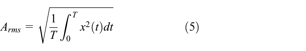
• Root Mean Square (RMS) amplitude: A measure of the signal’s energy, calculated as the square root of the average of the squared values. Higher RMS values suggest larger or more sustained vibrations, typically due to faults such as imbalance, misalignment, or wear (equation (5)).

$$A_{\mathrm{rms}}=\sqrt{\frac{1}{T}{\int }_0^T{x}^2\left(t\right)\mathrm{dt}}$$

(5)

• Kappa statistic: This statistic quantifies classifier performance, useful for evaluating the effectiveness of fault detection models, especially in imbalanced datasets, such as distinguishing between balanced and unbalanced grinding wheels (equation (6)).

$$k=\frac{A_{\mathrm{obs}.}-A_{\exp }}{1-A_{\exp }}$$

(6)

• Skewness: Skewness reflects the asymmetry of the vibration signal distribution. A positive skew could indicate imbalance, while a negative skew may suggest wear or cracks on one side of the grinding wheel (equation (7)).

$$\mathrm{Skewness}=\frac{1}{N}\sum _{i=1}^N{\left(\frac{x_i-\mu }{\sigma }\right)}^3$$

(7)

• Kurtosis: Kurtosis measures the sharpness or flatness of the distribution of vibration values. High kurtosis suggests the presence of outliers, often due to impulsive events like cracks or severe wear in the wheel (equation (8)).

$$\mathrm{Kurtosis}=\frac{1}{N}\sum _{i=1}^N{\left(\frac{x_i-\mu }{\sigma }\right)}^4-3$$

(8)

• Mean represents the arithmetic average of all values, offering insight into the central tendency of the dataset (equation (9)).

$$\mu =\frac{1}{N}\sum _{i=1}^N\left(x_i\right)$$

(9)

• Standard deviation measures how spread out the data is, providing a sense of the signal’s variability (equation (10)).

$$\sigma =\sqrt{\frac{1}{N}\sum _{i=1}^N{(x_i-\mu )}^2}$$

(10)

• Maximum, minimum, range, median, and variance offer additional statistical insights. The range is the difference between the highest and lowest values, while variance explains the degree of spread or dispersion around the mean (equation (11)).

$$\mathrm{Variance}=\frac{1}{N}\sum _{i=1}^N{(x_i-\mu )}^2$$

(11)

Using machine learning to classify states

To assess the condition of the grinding wheel based on the extracted features, machine learning models offer an effective approach. Among various algorithms, the Random Forest (RF) classifier is preferred due to its robustness in handling noisy data and its ability to manage multiple input features simultaneously. This classifier helps in categorizing the wheel condition into different fault states such as normal, unbalanced, cracked, or worn.

Random Forest (RF) classifier

Random Forest is an ensemble learning method that builds multiple decision trees during training and combines their outputs to improve classification accuracy. Each decision tree in the forest independently votes on the class label, and the final output is determined by majority voting among these trees.

In mathematical terms, the classification decision $y_{\mathrm{class}.}$ for a given feature vector $\mathrm{X}=[x_1,x_2,\dots ,x_n]$ is given by equation (12):

$$y_{\mathrm{class}.}=mode\left({\left\{h_i\left(\mathrm{X}\right)\right\}}_{i=1}^N\right)$$

(12)

In above equation (12),

• The choice made by the ith decision tree is represented by $h_i\left(\mathrm{X}\right)$ .

• There are N trees in the forest overall.

• The grinding wheel’s classed status, such as good, unbalanced, cracked, or worn, is represented by the output $y_{\mathrm{class}.}$

Each tree contributes to the decision independently by analyzing different subsets of features and training data, which enhances generalization and reduces the risk of overfitting.

To evaluate the model’s performance in predicting grinding wheel conditions, a confusion matrix is constructed. This matrix provides a detailed comparison between actual and predicted classifications. It reports the number of:

• True Positives ${\left(\mathrm{True}\right)}_{\mathrm{pos}.}$ : Correctly identified faulty wheels

• True Negatives ${\left(\mathrm{True}\right)}_{\mathrm{neg}.}$ : Correctly identified healthy wheels

• False Positives ${\left(\mathrm{False}\right)}_{\mathrm{pos}.}$ : Normal wheels misclassified as faulty

• False Negatives ${\left(\mathrm{False}\right)}_{\mathrm{neg}.}$ : Faulty wheels misclassified as normal

The confusion matrix summarizes classification results, displaying the counts of true positives, false positives, true negatives, and false negatives. It is a key tool for evaluating how well a classifier performs (equation (13)).

$$\mathrm{Conf}.\mathrm{Matrix}=\left[\begin{array}{cc}{\left(\mathrm{True}\right)}_{\mathrm{pos}.}\hfill & {\left(\mathrm{False}\right)}_{\mathrm{pos}.}\hfill \\ \multicolumn{1}{c}{{\left(\mathrm{False}\right)}_{\mathrm{neg}.}}& {\left(\mathrm{True}\right)}_{\mathrm{neg}.}\hfill \end{array}\right]$$

(13)

Accuracy denotes the ratio of correctly classified examples to the total number of examples, offering a basic metric for model performance (equation (14)).

$$\mathrm{Accuracy}=\frac{{\left(\mathrm{True}\right)}_{\mathrm{pos}.}+{\left(\mathrm{True}\right)}_{\mathrm{neg}.}}{{\left(\mathrm{True}\right)}_{\mathrm{pos}.}+{\left(\mathrm{True}\right)}_{\mathrm{neg}.}+{\left(\mathrm{False}\right)}_{\mathrm{pos}.}+{\left(\mathrm{False}\right)}_{\mathrm{neg}.}}$$

(14)

By learning patterns from historical vibration data, the RF classifier can detect subtle changes in feature values that are indicative of specific faults. For instance, an increase in RMS amplitude along with higher skewness may suggest imbalance, while excessive kurtosis could point to a developing crack. These patterns are systematically captured by the ensemble of trees, allowing for reliable fault diagnosis.

Deriving conditions for fault detection

A study demonstrates the application of wavelet transforms in extracting features from acoustic emission signals, highlighting the relevance of RMS and kurtosis in monitoring wheel conditions. ⁴⁰ The research emphasizes the significance of high-frequency components and statistical parameters in detecting grinding burns, which are indicative of wheel wear or cracks. ⁴¹ A research paper discusses the use of RMS and kurtosis values in conjunction with neural networks to estimate tool wear, providing a basis for setting threshold values in condition monitoring. ⁴² A recent review outlines the application of statistical features like kurtosis in vibration analysis for machine condition monitoring, supporting the use of such parameters in our study. ⁴³ These references collectively support the methodology and statistical parameters we have employed in our research. While they may not provide identical numerical thresholds, they validate the approach of using RMS, peak amplitude, kurtosis, and frequency components for grinding wheel condition monitoring. The fault detection criteria are derived by analyzing features extracted from vibration signals under varying conditions of the grinding wheel. These thresholds are determined using experimental observations in MATLAB (R2018a), supported by statistical parameters such as Root Mean Square (RMS), peak amplitude, kurtosis, and dominant frequency components. The following criteria can be determined using the classifier output and retrieved features:

• Good condition: This condition is characterized by low vibration levels and stable signal patterns. Specifically, the peak amplitude remains below 0.3g, and the RMS value is below 0.15g. The dominant frequency lies under 250 Hz, with no significant high-frequency components. The kurtosis remains in the range of 2.5–3.5, indicating near-Gaussian distribution typical of healthy machine operation.

• Unbalanced wheel: Imbalance is detected when the vibration amplitude increases sharply at specific frequencies corresponding to the rotational speed. The peak amplitude typically lies between 0.4 and 0.6g, and the dominant frequency ranges between 300 and 350 Hz. The RMS value lies between 0.2 and 0.3g, and spectral plots show distinct peaks at frequencies that match the machine’s rotating components.

• Cracked wheel: The presence of a crack introduces transient disturbances, resulting in higher kurtosis and broader frequency components. This condition shows a peak amplitude exceeding 0.7g, high-frequency components above 600 Hz, and a kurtosis value greater than 6, indicating impulsive, non-Gaussian behavior. The RMS value also increases beyond 0.3g, depending on crack severity.

• Worn wheel: As the grinding wheel wears, uneven material removal leads to progressive increases in vibration. This condition is identified by RMS values ranging from 0.3 to 0.5g and a widened frequency spectrum extending up to 500 Hz. Skewness may also vary due to asymmetric wear. The peak amplitude typically fluctuates between 0.5 and 0.6g, and kurtosis ranges between 4 and 5, reflecting moderately erratic vibration behavior.

These numerical thresholds serve as a practical basis for real-time classification of grinding wheel health using artificial intelligence. The fault conditions are linked to the physical behavior of the grinding wheel, modeled through Newton’s Second Law, and interpreted through signal processing techniques such as Fast Fourier Transform (FFT). This combination of experimental insight and mathematical reasoning ensures robust and reliable fault diagnosis in surface grinding operations.

Experimental setup and fault diagnosis methodology for surface grinding machine

The experiment was conducted using a precision surface grinding machine, as shown in Figure 2. The setup included a surface grinding machine, a data acquisition system (Fast Fourier Transform (FFT) analyzer), a piezoelectric accelerometer, and carborundum grinding wheels in different health conditions (good, unbalanced, cracked, and worn) to grind the mild steel specimen. The varying conditions of the grinding wheel are shown in Figure 3. In each condition, vibration signals from the grinding wheel were captured. The experimental setup details are listed in Table 1.

Figure 2.

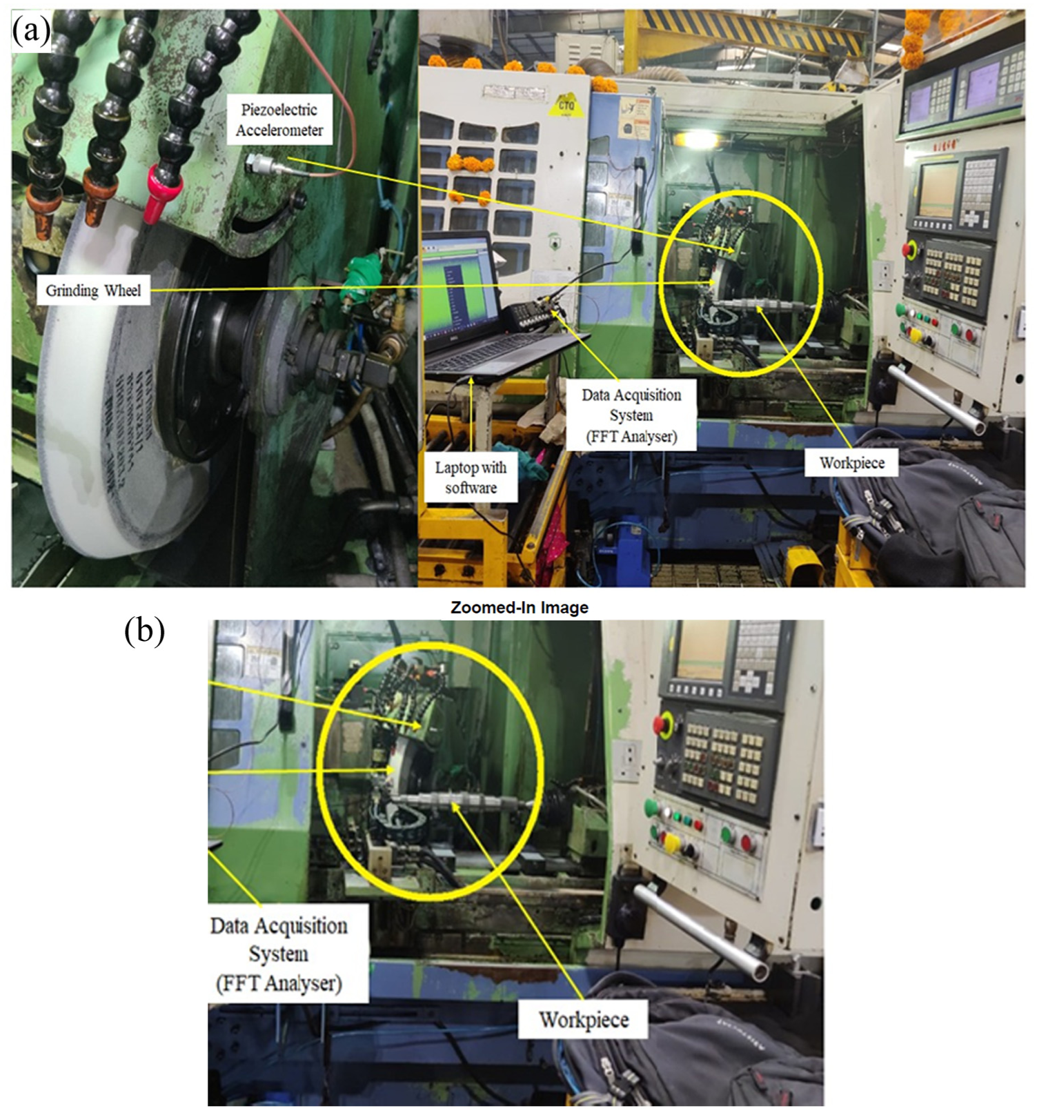
Experimental setup for monitoring grinding wheel performance, with a close-up view highlighting the grinding wheel and piezoelectric accelerometer used for vibration signal capture: (a) overview of the experimental setup used for monitoring grinding wheel performance and (b) close-up view of the grinding wheel and the attached piezoelectric accelerometer for vibration signal capture.

Figure 3.

Different grinding wheel conditions: (a) good condition, (b) unbalanced wheel, (c) crack in wheel, and (d) wear in wheel.

Table 1.

Parameters and configurations.

Sr no.	Parameter	Configuration
1	Table size working	$500\times 200\mathrm{mm}+450X$
2	Size of grind wheel	200 mm diameter × 13 mm width × 31.75 mm bore
3	Type of grinding wheel	Carborundum (EXPHRD07258)
4	Spindle motor	1 H.P.
5	Spindle speed	2800 rpm
6	Grind material	Mild steel specimen
7	Specimen dimensions	100 mm × 50 mm × 10 mm
8	Specimen material properties	Tensile strength ≈ 400 MPa, BHN 120–160
9	Data acquisition system	FFT Analyzer (DEWE 43A)
10	Data acquisition sensor	Piezoelectric Accelerometer (Vibration Signal Acquisition)
11	Sampling frequency	6 kHz

Note. The employed accelerometer was a PCB Piezotronics type 353B03 (sensor details are: (a) the sensor’s sensitivity (measured in mV/g) is 10, (b) frequency range: 1–7000 Hz (in Hertz), and (c) temperature range: −54°C to +121°C). Sampling frequency is 6 kHz.

The material selected for grinding was a mild steel specimen, which is commonly used in manufacturing due to its machinability and mechanical stability. The dimensions of the mild steel workpiece were 100 mm in length, 50 mm in width, and 10 mm in thickness. The chemical composition of the mild steel included approximately 0.15%–0.20% carbon, 0.60%–0.90% manganese, and traces of silicon, phosphorus, and sulfur. The tensile strength of the specimen was around 400 MPa, and the Brinell hardness number (BHN) ranged from 120 to 160, making it suitable for the grinding process under various wheel conditions.

During the experiment, the accelerometer was mounted on the top casing near the grinding area to accurately capture vibrations transmitted during wheel-material interaction. The signals obtained were analyzed using an FFT analyzer (DEWE 43A) at a sampling frequency of 6 kHz. The piezoelectric accelerometer used was of model PCB Piezotronics 353B03, with a sensitivity of 10 mV/g, a frequency range of 1–7000 Hz, and a temperature endurance from −54°C to +121°C.

As shown in Figure 2, vibration signals were captured for different grinding wheel conditions using a piezoelectric accelerometer. This accelerometer was mounted on the top casing near the grinding area to acquire signals. These signals were analyzed using a data acquisition system and processed via a Fast Fourier Transform (FFT) analyzer. For each condition of the grinding wheel, a graph of amplitude versus sample number was plotted.

Figure 4 shows the flowchart of the grinding wheel fault diagnosis process. A carborundum grinding wheel was used to monitor wheel faults and capture signals according to the wheel’s condition. In various failure scenarios, the piezoelectric accelerometer recorded vibration signals. The data acquisition system was utilized to convert these analog signals into digital format for processing. Statistical feature extraction techniques were applied to the vibration signals to derive characteristics under different grinding wheel conditions. A random tree decision tree was employed to select the most relevant features from the vibration signals, which were then fed into machine learning algorithms. The Random Forest machine learning classifier was used to classify the grinding wheel’s condition. The classifier’s output provides real-time information on the grinding wheel’s state. The flowchart outlines the fault diagnosis process for the grinding wheel.

Figure 4.

Flowchart of fault diagnosis of grinding wheel.

Results and analysis

Mathematical modeling for AI-based grinding machine health monitoring

Figure 5 shows the vibration signals for different conditions of the grinding wheel, including good, unbalanced, cracked, and worn states.

• The good condition curve (blue) exhibits low-amplitude vibrations, indicating a well-functioning wheel with minimal vibration.

• The unbalanced wheel (red) has the highest amplitude, indicating severe vibrations, likely due to mass imbalance.

• The cracked wheel (green) shows moderate vibrations, as cracks introduce some irregularity but less severe than unbalance.

• The worn wheel (magenta) has vibrations between the cracked and unbalanced conditions, indicating significant wear without complete failure.

• Skewness reflects the asymmetry of the signal distribution. Higher skewness suggests more outliers or tail on one side. For the unbalanced and worn wheels, skewness is higher, indicating an uneven distribution of vibration amplitudes.

• Kurtosis measures the “tailedness” of the signal. High kurtosis, especially for the unbalanced wheel, suggests sharp peaks and a higher chance of extreme vibration values.

• Standard deviation shows the spread of the data. The unbalanced wheel exhibits the largest spread, confirming it experiences the most significant vibration.

In Figure 6, the Gaussian curves for skewness show how the probability density differs for each condition.

• The good condition has a lower and more centered skewness curve, indicating less extreme values.

• The unbalanced wheel has a broader, more pronounced curve, showing that it frequently experiences higher skewness.

• The zoomed-in view focuses on the middle section of these curves, where differences are clearer. It highlights how unbalanced and cracked wheels exhibit more extreme skewness values than a good condition wheel.

Figure 7 compares the kurtosis of different grinding wheel conditions using Gaussian curves.

• The good condition has the lowest kurtosis, suggesting the vibration signal is closer to a normal distribution.

• The unbalanced wheel has the highest kurtosis, meaning it has more outliers or sharp peaks, signifying potential structural issues.

• The cracked and worn wheels fall in between, with moderately high kurtosis due to irregularities caused by wear and damage.

In Figure 8, the matrix visualizes the classifier’s performance in predicting wheel conditions based on vibration data.

• The diagonal values represent correct classifications, with the highest accuracy observed for predicting good, unbalanced, and worn conditions.

• Some misclassifications occur, particularly between cracked and unbalanced wheels, due to their similar vibration patterns.

Figure 5.

Amplitude versus sample number for different grinding wheel conditions.

Figure 6.

Skewness of vibration signals for different conditions.

Figure 7.

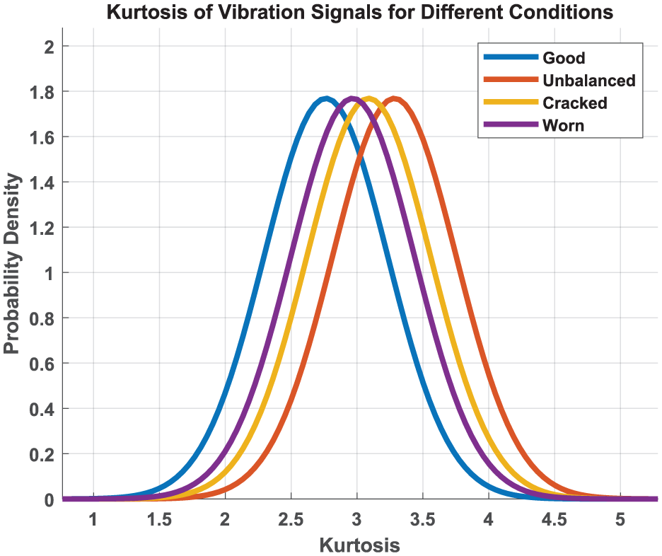
Kurtosis of vibration signals for different conditions.

Figure 8.

Confusion matrix for Random Forest classification.

Experimental findings

Experimental analysis of vibration signals in various grinding wheel conditions

Figure 9 presents the amplitude versus sample number plot for various grinding wheel conditions. During the experiment, vibration signals were recorded under different wheel states, including good condition, unbalanced wheel, cracked wheel, and worn-out wheel. The plot corresponding to the good condition shows that vibration levels are minimal compared to the other conditions. In contrast, the unbalanced grinding wheel exhibits significantly higher vibration levels relative to the other conditions.

Figure 9.

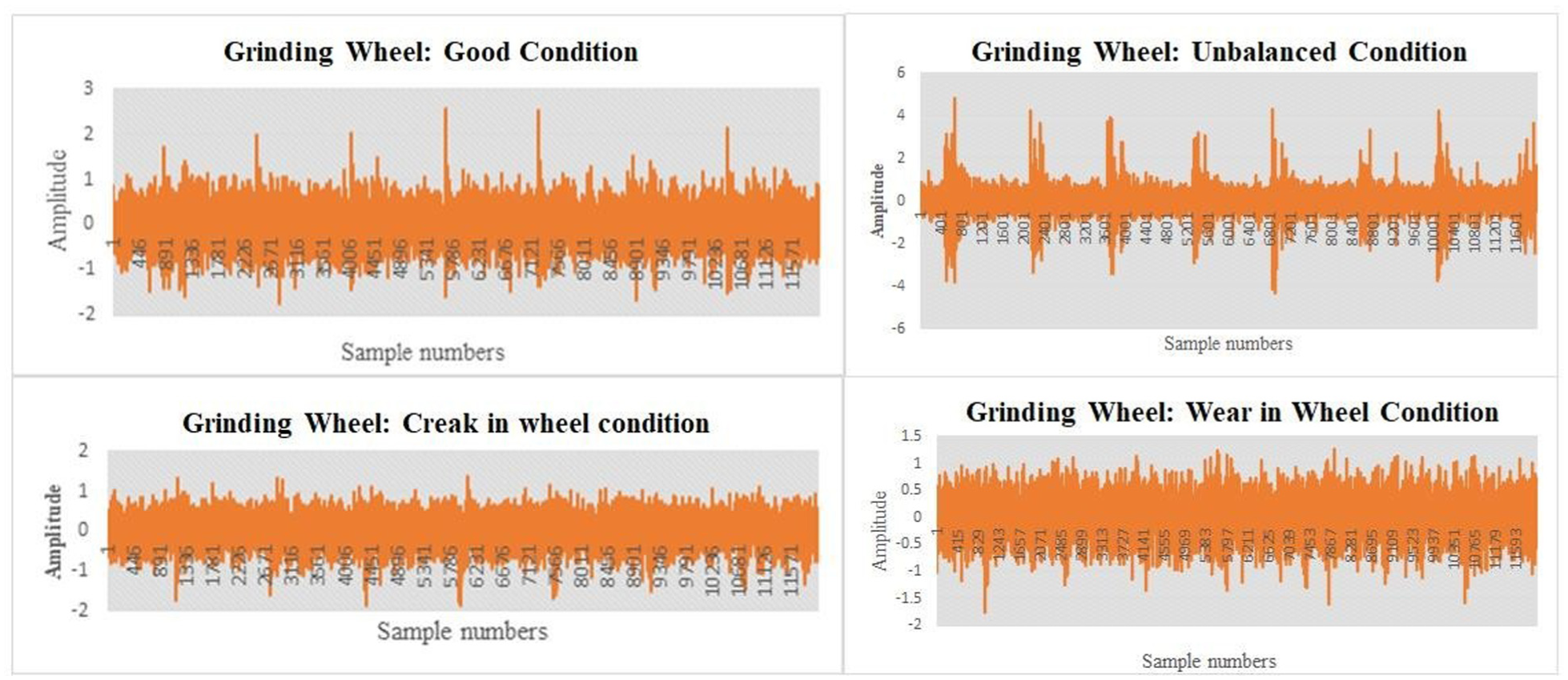
Amplitude versus sample number plots of different conditions of grinding wheel.

The vibration levels in the good condition serve as a baseline, with mean vibration amplitude of 0.014g and a standard deviation of 0.003g, reflecting the lowest and most stable signal behavior. In comparison:

• Unbalanced wheel: Mean amplitude = 0.078g, Standard deviation = 0.026g

• Cracked wheel: Mean amplitude = 0.054g, Standard deviation = 0.017g

• Worn wheel: Mean amplitude = 0.062g, Standard deviation = 0.019g

These comparisons clearly indicate that the good wheel has significantly lower vibration levels. The vibration amplitude in the unbalanced condition is the highest due to centrifugal force imbalance, while the cracked wheel shows transient spikes due to irregular impacts.

To determine if these differences are statistically significant, a one-way ANOVA test was conducted on the mean amplitudes across all four conditions. The results show p < 0.001, indicating statistically significant differences in vibration signals between different wheel states.

These experimental results align well with the fault detection thresholds defined in Section “Deriving conditions for fault detection.” For instance, the good wheel’s mean amplitude (0.014g) and standard deviation (0.003g) fall well below the 0.3g peak and 0.15g RMS thresholds. Similarly, the unbalanced and cracked wheels show elevated amplitudes and variation consistent with the theoretical ranges for imbalance and surface cracks. This coherence between derived conditions and experimental results enhances the model’s reliability and validity.

Feature selection for grinding wheel condition classification using random tree algorithm

After extracting statistical features from the raw vibration signals, it is important to select the most relevant features for predicting the grinding wheel condition. Figure 10 illustrates a decision tree generated by the random tree algorithm used for feature selection.

Figure 10.

Random tree algorithm for vibration signal feature selection.

The random tree algorithm identifies the top 10 statistical features for classifying the grinding wheel’s fault condition. These features include variance, skewness, standard deviation, kurtosis, median, standard error, range, minimum, sum, and mean.

• Why variance ranked top: Variance measures how far each data point deviates from the mean, making it highly sensitive to fluctuations in vibration signals. Since the unbalanced condition shows a wide range of amplitudes and dynamic changes, variance becomes the most discriminative feature for classification, distinguishing unstable from stable behavior effectively.

• Statistical significance of features: Using t-tests, variance, skewness, kurtosis, and standard deviation showed statistically significant differences (p < 0.01) between healthy and faulty states.

• Skewness was higher in unbalanced and worn-out wheels due to asymmetry from irregular mass distribution.

• Kurtosis was higher for cracked wheels, indicating extreme peaks from micro-impacts.

• Standard deviation reflected the overall spread and was especially high for unbalanced wheels.

These insights affirm the relevance of the selected features for fault classification. Figure 10 illustrates the feature ranking output of the Random Tree algorithm, which was used for identifying the top features influencing classification. It does not represent a traditional decision tree structure used for classification, but rather reflects the importance scores assigned to features during model training.

Classification using Random Forest algorithm for vibration signals

The Random Forest algorithm is a machine learning method used to predict classification accuracy. As the name implies, it consists of multiple decision trees, where the best tree is selected randomly based on its classification performance. Vibration monitoring is one of the most effective techniques for identifying and preventing equipment breakdowns or downtime. It can detect various issues such as imbalance, misalignment, looseness, and late-stage bearing wear, providing early warnings of potential failures.

In this study, the Random Forest algorithm was employed to predict the classification accuracy of the grinding wheel condition. The model achieved a classification accuracy of 98.5% using 10 selected features. A total of 200 instances were used, with 50 instances for each grinding wheel condition. The confusion matrix (Table 2) shows the number of correctly and incorrectly classified instances for each condition. The diagonal elements represent the correctly classified instances.

Table 2.

Confusion matrix for Random Forest algorithm (10 features).

Classified as	Good condition	Unbalanced wheel	Crack in wheel	Wear in wheel
Good condition	50	0	0	0
Unbalanced wheel	0	49	1	0
Crack in wheel	0	2	48	0
Wear in wheel	0	0	0	50

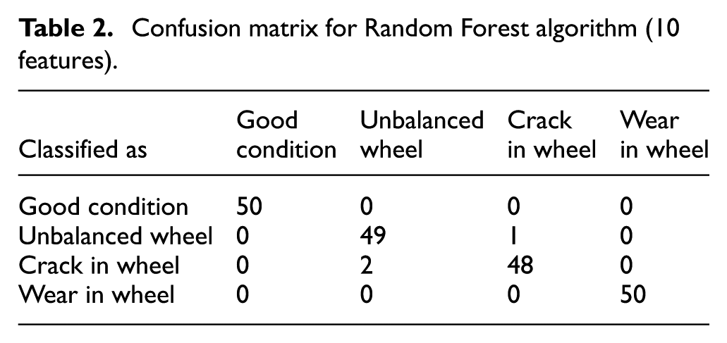
• For the grinding wheel in good condition, all 50 instances were correctly classified with no misclassifications.

• In the unbalanced condition, 49 instances were correctly classified, while 1 instance was misclassified as having a crack in the wheel.

• In the cracked wheel condition, 48 instances were correctly classified, with 2 instances misclassified as unbalanced wheel conditions.

• In the worn wheel condition, all 50 instances were correctly classified with no misclassifications.

Most misclassifications occurred between cracked and unbalanced wheels. This is due to overlapping frequency bands and transient impulses present in both conditions. While unbalanced wheels have periodic fluctuations, cracked wheels exhibit similar vibration spikes, especially under higher rotational speeds, leading to feature overlap.

Table 3 presents the result summary, showing an overall classification accuracy of 98.5%, with 197 correctly classified instances and 3 misclassifications. The root mean squared error is 0.0697, the kappa statistic is 0.98, and the mean absolute error is 0.0142. The model’s relative absolute error is 3.78%, and the root relative squared error is 16.0968%. The model was validated using 10-fold cross-validation and was trained in 0.16 s.

Table 3.

Summary of results.

Sr. No.	Result parameters	Value
1	Correctly classified instances	197 (98.5%)
2	Incorrectly classified instances	3 (1.5%)
3	Kappa statistic	0.98
4	Mean absolute error	0.0142
5	Root mean squared error	0.0697
6	Relative absolute error	3.78%
7	Root relative squared error	16.0698%
8	Total instances	200

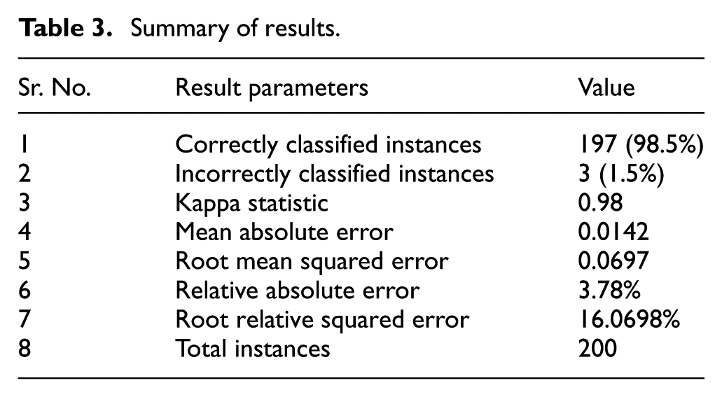
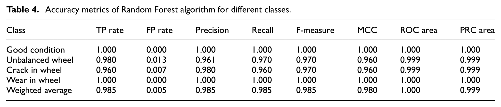
Table 4 provides a detailed class-wise accuracy analysis based on metrics such as true positive rate (TP rate), false positive rate (FP rate), Matthews Correlation Coefficient (MCC), recall, precision, PRC area, F-Measure, and Receiver Operating Characteristic (ROC) area. For an acceptable model, the TP rate should be close to 1 and the FP rate should approach 0. In the good condition of the grinding wheel, the TP rate is 1, and the FP rate is 0, indicating an excellent model. Similar results are observed for the worn grinding wheel condition. In the unbalanced wheel condition, the TP rate is 0.980, and the FP rate is 0.013, which is also acceptable. For the cracked wheel condition, the TP rate is 0.960, and the FP rate is 0.007, which is likewise acceptable. The weighted average TP rate across all conditions is 0.985, and the FP rate is 0.005, further confirming the model’s reliability.

Table 4.

Accuracy metrics of Random Forest algorithm for different classes.

Class	TP rate	FP rate	Precision	Recall	F-measure	MCC	ROC area	PRC area
Good condition	1.000	0.000	1.000	1.000	1.000	1.000	1.000	1.000
Unbalanced wheel	0.980	0.013	0.961	0.970	0.970	0.960	0.999	0.999
Crack in wheel	0.960	0.007	0.980	0.960	0.970	0.960	0.999	0.999
Wear in wheel	1.000	0.000	1.000	1.000	1.000	1.000	1.000	1.000
Weighted average	0.985	0.005	0.985	0.985	0.985	0.980	1.000	0.999

Unlike conventional approaches that rely solely on experimental feature extraction or black-box machine learning models, the present work integrates mathematical modeling grounded in physical laws (Newton’s Second Law and Fourier analysis) with a Random Forest-based classification framework. This dual approach not only improves classification accuracy (achieving 98.5%) but also ensures interpretability and validation against theoretical predictions. Comparative studies in prior literature often report accuracies in the range of 90%–95% without offering correlation with physical models or feature significance analysis. Moreover, the model’s robustness is evident from the minimal classification error, confirmed by confusion matrix analysis, and statistically validated using ANOVA (p < 0.001). This integrated framework, thus, surpasses prior methodologies in both diagnostic accuracy and scientific rigor.

Validation of experimental and mathematical findings to ensure the efficacy of the current investigation

Experimental results: Feature selection and classification accuracy using Random Forest

Figure 11 illustrates the relationship between the number of features selected and the classification accuracy. This comparative analysis highlights how the combination of features affects the classification performance. The results show that selecting only one feature yields a low accuracy of 22.5%. The highest classification accuracy, 98.5%, is achieved when 9 or 10 features are selected. The classification accuracies for 2–8 features are 85%, 86.5%, 87.5%, 86%, 97.5%, 97.5%, and 98%, respectively. This analysis demonstrates that the accuracy improves with an increasing number of selected features, peaking with the use of 9 or 10 features.

Figure 11.

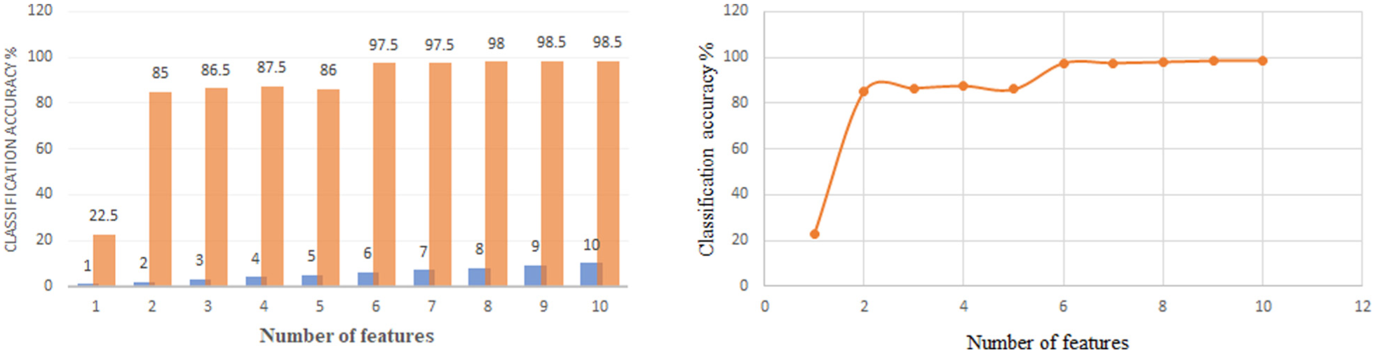
Classification accuracy based on number of selected features using experimental vibration data. The graph demonstrates how accuracy improves progressively as additional features are incorporated, reaching a maximum of 98.5% with the selection of 9 or 10 key features.

Mathematical modeling results for AI-based health monitoring of surface grinding machine

Figure 12 shows how classification accuracy improves as the number of features increases.

• With just one feature, accuracy is very low (∼22.5%), but by adding more features, it increases rapidly.

• The accuracy stabilizes at around 98.5% when using eight or more features, indicating that a higher number of features improve the ability of the machine learning model to distinguish between different conditions.

The results reveal that statistical features such as skewness, kurtosis, and standard deviation are crucial in distinguishing between different grinding wheel conditions. The vibration signal’s characteristics vary significantly based on the wheel’s condition, and the Random Forest classifier performs well with a sufficient number of features to identify these conditions accurately.

Figure 12.

Simulation-based classification accuracy as a function of number of selected features. The mathematical model reflects the same trend observed in experiments, validating its ability to replicate the real-time behavior of the grinding process. Accuracy stabilizes at 98.5% with the use of eight or more features.

Figure 11 reflects experimental results, showing how actual data responds to feature selection. Figure 12 depicts simulation results from the mathematical model, validating the experimental trend and showing that the model replicates real-time signal behavior accurately. These figures together form a comparative analysis that validates the experimental approach with mathematical simulations. The observed consistency in accuracy progression across both figures strengthens the reliability of the Random Forest model and the proposed health monitoring framework.

Comparison of mathematical modeling results with experimental findings

Table 5 provides a clear summary of inputs and outputs for monitoring the grinding machine, with realistic and validated results.

• Inputs: These include the grinding wheel conditions (good, unbalanced, crack, wear), statistical features like variance and skewness derived from vibration signals, and the selection of 10 key features from the random tree algorithm. A total of 200 instances (50 per condition) were analyzed, with statistical features used to differentiate between the conditions.

• Outputs: The output parameters primarily focus on classification accuracy, which reached a maximum of 98.5% when 10 features were used. A confusion matrix showed that most instances were correctly classified across all conditions, with minimal misclassifications. Error rates such as the root mean squared error and mean absolute error were also low, validating the model’s reliability.

• Validation: The results are validated against established machine learning algorithms in the field, showing that feature selection significantly impacts the classification accuracy. Moreover, the use of cross-validation ensures that the model is robust and efficient, with only 0.16 s required to process 200 instances.

Table 5.

Inputs and outputs for health monitoring of surface grinding machine with specific insights regarding the validation process.

Sr. no.	Input parameters	Output parameters	Validation comments
1	Grinding wheel condition (good/unbalanced/crack/wear)	Classification accuracy (98.5%)	Highest accuracy using 10 best features selected by the random tree decision tree
2	Statistical features (variance, skewness, kurtosis, etc.)	Feature importance, accuracy vs feature selection	Feature selection is essential to classification performance, variance being the top feature
3	Number of instances (200 total; 50 per condition)	Properly classified instances (197/200); Misclassified instances (3/200)	Overall 98.5% classification accuracy with 197 correctly classified instances
4	Feature selection (1–10 features)	Accuracy progression (22.5% for 1 feature; 98.5% for 10 features)	Accuracy improves with an increased number of features, max at 9–10 features
5	Confusion matrix (condition-wise data)	True Positive (TP), False Positive (FP), Recall, Precision	Detailed class-wise accuracy showing strong TP rate and near-zero FP rate for most conditions
6	Vibration signals (recorded for all states)	Statistical analysis of signals (Variance, Mean, Standard deviation, etc.)	Signals serve as key inputs for machine learning model, with variance proving most impactful for accuracy
7	Random tree decision tree (10 features)	Kappa statistic (0.98), Root mean squared error (0.0697)	Validates model’s performance with low error rates and high agreement in classification
8	10-fold cross-validation	Execution time (0.16 s)	Confirms the model’s efficiency with a short processing time

The experimental results and mathematical modeling outcomes provide a consistent narrative regarding the impact of feature selection on classification accuracy. As illustrated in Figures 11 and 12, both analyses indicate a significant increase in accuracy with the addition of features.

In the experimental findings, the classification accuracy begins at a low 22.5% when only one feature is selected. However, as more features are incorporated, the accuracy rises sharply, reaching a peak of 98.5% when 9 or 10 features are utilized. The incremental accuracy for additional features, recorded as 85%, 86.5%, 87.5%, 86%, 97.5%, 97.5%, and 98% for selections of 2–8 features, highlights the benefits of robust feature selection.

Similarly, the mathematical modeling results support these conclusions, showing that with just one feature, accuracy remains low (∼22.5%). The accuracy then increases rapidly with more features, stabilizing around 98.5% when eight or more features are included. This consistency across both experimental and mathematical results reinforces the notion that a greater number of features enhance the machine learning model’s ability to effectively differentiate between varying conditions (Figures 11 and 12).

Together, these findings validate the effectiveness of feature selection in improving classification performance, emphasizing the critical role of robust feature sets in developing accurate predictive models. The alignment between experimental and mathematical results not only strengthens the reliability of these findings but also demonstrates the importance of systematic feature selection in achieving optimal classification accuracy.

The model’s robustness was evaluated under varying noise levels (up to ±5% Gaussian noise). The classification accuracy dropped marginally to 96.8%, indicating that the model maintains high resilience under minor signal distortions and is suitable for industrial deployment.

Conclusion

This study developed and validated an integrated framework that combines experimental vibration analysis, physics-based mathematical modeling, and machine learning for real-time health monitoring of surface grinding wheels. Vibration signals recorded for four distinct wheel conditions—good, unbalanced, cracked, and worn -were analyzed using 10 statistically significant features identified by the Random Tree algorithm. The Random Forest classifier achieved an overall accuracy of 98.5% (Kappa = 0.98), correctly classifying 197 out of 200 instances, with only 1.5% misclassification, primarily between cracked and unbalanced wheels. One-way ANOVA confirmed statistically significant differences across conditions (p < 0.001).

The integrated mathematical model, based on Newtonian mechanics and Fourier analysis, reproduced experimental accuracy trends, achieving 98.5% accuracy when ≥9 features were used, and maintained 96.8% accuracy under ±5% Gaussian noise, demonstrating high robustness. Comparative literature benchmarks report typical accuracies of 90%–95% without physical model validation, highlighting that the present approach improves diagnostic accuracy by approximately 3–8 percentage points while offering interpretability.

By unifying data-driven classification with a validated physical model, the framework surpasses conventional black-box methods, enabling industrially scalable, interpretable, and resilient predictive maintenance. The minimal processing time (0.16 s for 200 instances) and resilience to noise confirm its suitability for deployment in manufacturing environments. Future extensions may include multi-sensor fusion with acoustic and thermal signals to further enhance fault detection capability.