
Abstract
The quality of measured responses in terms of displacement or deformation plays an important role in structural health monitoring (SHM). The aim of this article is to identify the impact force that takes the form of a moving signal, such as the passage of trains and vehicles over a bridge. The structure considered in this work is a beam resting on elastic and/or rigid supports, the aim of which is to study the influence of the moving force while taking into account different support conditions. The effect of sensor position on reconstruction quality will be discussed in this article. Since the inverse problem is ill-posed, regularization methods are essential. The Tikhonov-SVD technique is considered in this work. This regularization technique will be tested by adding noise to the measured responses.
Keywords
Introduction
The study of impact forces on structures is very essential to understanding their dynamic behavior under instantaneous loads, especially when the structure is under dynamic forces. In this context, beams are among those basic structural elements that play a vital role in many civil engineering structures in terms of load transfer and dissipation. When beams are subjected to dynamic loads, such as those caused by vehicles and trains crossing a bridge or machinery working inside a factory, understanding the actions of such loads on their structural integrity and strength becomes a must. The study of the influence of a moving force applied to a beam includes the description of the dynamics related to the motion of the force along the structure and consideration of the support conditions of the beam, which can be either rigid or elastic.1–5 These two different classes of supports significantly affect the force distribution and the dynamic response of the beam.
Rigid supports are those that will not allow any form of deformation, 6 hence providing infinite rigidity. On the other hand, the elastic supports do allow some amount of deformation once an external load is applied to them.7,8 Battini and Ülker-Kaustell 6 proposed an approach to study the nonlinear influence of ballast in vertical dynamic analyses of railway bridges for a beam sitting on rigid supports. Liao et al. 7 used fiber Bragg grating (FBG) sensors to collect deformation data, enabling the construction of neural networks. A comparison was made between the data collected by FBG and that obtained using the finite element method. Moliner et al. 8 proposed a solution that relies on the modernization of the bridge with a set of discrete viscoelastic dampers (VED) connected to the slab and to an auxiliary structure, placed under the bridge deck and resting on the abutments. Yu and Chan 9 presented the study focused on time-frequency domain to identify an axle force acting the bridge with rigid support. Studying the reaction of a beam under these two support conditions is an integral part of analyzing its capacity to absorb impact forces, which could either be concentrated forces at a given point or forces that travel along the length of the beam.10–12 The importance of this study is even more significant in areas where the structures’ safety and durability are paramount.
The identification of impact forces is a fundamental technique in structural health monitoring (SHM). It allows for the assessment of structural damage by detecting and quantifying the applied forces. Typically, this technique relies on the inversion transfer matrix, which encapsulates the dynamic and mechanical properties of materials. However, this inversion is highly sensitive to even minor perturbations in the transfer matrix parameters, which can lead to unstable or physically inconsistent solutions. Zhu and Law 10 developed a method based on modal superposition and regularization techniques in order to identify the moving load. They studied the effect of different parameters, namely, the measurement noise, the vertical and rotational stiffness of the supports, as well as the speed of displacement of the forces. Zhang et al. 13 proposed an approach based on intelligent visual perception technology to identify a moving load occurring on bridges. They evaluated the efficiency and robustness of the identification method, which depended on the position of the cameras and the number of points required to reconstruct the impact force. He et al. 14 proposed a time-domain identification method using the finite element method (FEM), based on the second-order Taylor expansion. They discuss the sensitivity of the method to factors such as the number of sensors, noise, and vehicle speed.
In this context, the identification problem is known to be ill-posed, and solving this ill-posedness requires the use of regularization methods. 15 The utilization of regularization techniques is essential to ensure the stability of the resulting data. These methods, including Tikhonov regularization, truncated singular value decomposition (TGSVD),16–18 and other variants, help control the impact of perturbations on the obtained solutions. The effectiveness of these approaches has been demonstrated in various inverse problems.19,20 Qiao et al. 21 proposed a sparse regularization approach to solve the underdetermined problem of impact-force reconstruction. Pan et al. 22 identified a moving load using sparse regularization, considering a constraint of stable mean values for the time histories of moving forces. They discuss the uncertainty in dynamic responses due to sensor calibration errors.
It is therefore essential to select appropriate regularization techniques and test their robustness against disturbances and noise to ensure reliable identification of the impact force. Sensor measurements are often affected by external interference or internal disturbances, such as electromagnetic noise or calibration errors, which degrade the quality of recorded data.23–25 Such disturbances complicate the accurate reconstruction of the impact force, leading to reduced reliability of the results. To address these challenges, the study employs regularization methods to filter out noise and preserve the integrity of the reconstruction.
This research is crucial for the field of structural health monitoring (SHM), where the precision of impact force measurements and the ability to minimize disturbances are vital for ensuring the safety and functionality of structures. The primary objective of this study is to examine how sensor placement and regularization methods influence the precision of impact force history reconstruction in beams. Additionally, the study investigates the optimal sensor placement configuration, considering the propagation of elastic waves through the structure, and evaluates the effect of noise on the reconstruction process. The study also explores the impact of excitation frequency and the effect of the stiffness of the elastic support.
Theory of moving load identification
Dynamic behavior of structure
A homogeneous and isotropic elastic beam with a uniform rectangular cross-section is considered. The beam has length L, width b, and height e, and its mechanical properties are characterized by the Young’s modulus E and the Poisson’s ratio
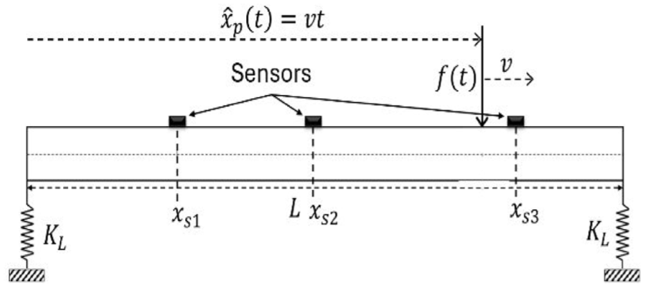
An elastic beam with a uniform rectangular cross-section, elastically supported and subjected to a moving load.
Based on the above hypotheses, the transverse displacement of the beam occurs in the vertical plane of symmetry. Taking into consideration the damping effect, the Euler–Bernoulli model describing the transient dynamic response of the beam following an impact is given by the following equation:

Where
The corresponding boundary conditions, defined in terms of displacement and its derivatives with respect to the spatial coordinate
Rigid supports:

Elastic supports:

Expressing the transverse displacement

where

where

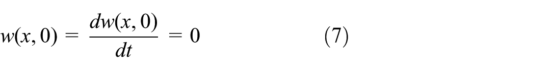
This is a second-order linear differential equation with a second member. Given the initial conditions at rest, these can be expressed as follows:
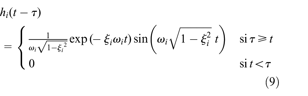
The general solution of differential equation (5) is given by the following Duhamel integral:

where:
The eigenvalue problem’s solution
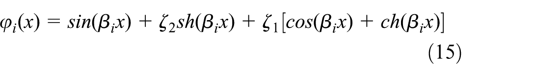
The general expression for the eigenfunction of the Euler-Bernoulli beam is given as:

where

For a beam with rigid supports, the eigenvalue and eigenfunction are expressed as follows 26 :
The eigenvalue is defined as:

And the eigenfunction is defined as:

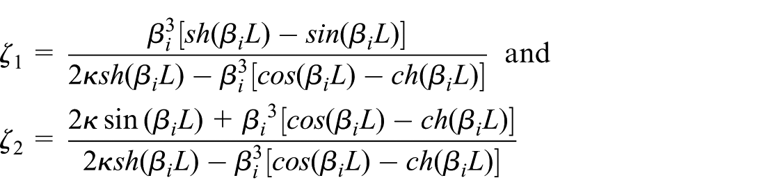
For a beam with elastic supports, the eigenvalue and eigenfunction are expressed as follows 5 :
The eigenvalue is the solution of the following equation:

where
where:
Identification of the moving load
The displacement of the beam at point x and time t can be found from equations (4) to (8) as:
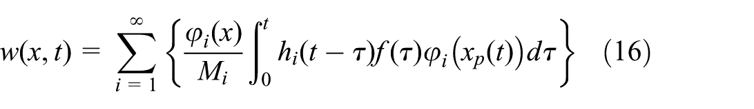
The strain in the beam at point x and time t can be written as:

Substituting equation (17) into equation (16) and rewriting it in matrix form gives:

with
where

Equation (18) can be rewritten in compact form as follows:

where
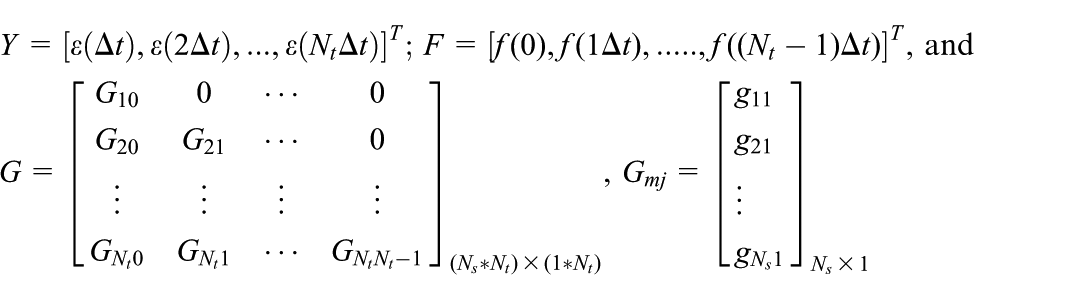
Where

Regularization
The transfer matrix G associated with the moving load acting on a beam is ill-conditioned, so we use Tikhonov’s method coupled with singular value decomposition (SVD) 19 to regularize it. This reformulates the ill-posed problem as a constrained optimization problem expressed as:

Where
By differentiating equation (22) and applying the optimality condition, which consists of setting this derivative to zero, we obtain the modified normal equation. This equation provides a mathematically rigorous framework for solution stabilization and is written as follows:

The technique employs the singular value decomposition (SVD) of the transfer matrix, expressed as

The filtering factors,
In this article, we will examine two selection methods,
The first is direct minimization of the mean square error called the S-curve error, 27 based on a comparison between the regularized force and the actual force applied, which allows us to plot an error curve S(λ) for different values of λ. This represents the relative error between the actual force and the regularized force, calculated as follows:

this method is limited by the requirement to know the actual values, which are often inaccessible in practical applications. The second, called generalized cross-validation (GCV) criterion, 28 based on statistical considerations and on the qualities of the solution prediction in relation to the data. A good value of the regularization parameter should predict missing values. This predictive method seeks to minimize the mean square error of estimation. The GCV function is defined as follows:

Where
Simulation and results
Numerical verification of the proposed approach was performed on an aluminum beam having the following parameters: length

Direct problem analysis
Analysis of the frequency response function (FRF) enables us to assess the impact of boundary conditions, such as rigid or elastic supports, on the dynamic behavior of a structure. Figure 2 shows that, in the case of rigid supports, the response is dominated by a marked resonance peak around 56 Hz, concentrating vibratory energy at low frequencies. Conversely, for elastic supports, a second major peak appears around 350 Hz, revealing the effect of the support’s flexibility, which introduces higher natural frequencies and a broader response. This comparison shows that the nature of the support influences not only resonance amplitudes but also the distribution of vibratory modes in the frequency spectrum. It should be noted that the first resonance frequency, in the case of an elastically supported system, decreases significantly to 7 Hz. The Table 1 presents the different frequency values for the first 10 modes, whether for a rigid support or an elastic support.

Frequency response functions for rigid and elastic supports. (a) Rigid supports case, (b) elastic supports case.
The frequencies of the first 10 modes.

Effect of noise
The effect of noise on the measured response can be written in equation (28), which represents the proportionality of the standard deviation of the calculated response. To evaluate the sensitivity of the regularization method to noise, white noise is added to the calculated beam responses to simulate the contaminated measurements, and 0.5%, 1%, 3%, and 5% noise levels are examined separately:

where
The quality of regularization is assessed by calculating relative errors as follows 24 :

Table presents the results of a comparative study of S-curve and GCV methods for estimating the optimal regularization parameter (
The values of optimal regularization parameter and the relative errors RPE for each noise level by the S-curve method and the GCV method for both types of supports.

However, the RPE is systematically higher in the case of elastic supports compared to rigid supports, despite a better overall quality of force identification in the rigid configuration, as shown in the Figures 3 and 4. This disparity can be attributed to differences in initial boundary conditions. Indeed, for rigid supports, the initial deformation at time is zero, while the initial applied force is non-zero, which begins force identification from zero. In order to evaluate the effectiveness of the proposed approach on the quality of impact force reconstruction, three regularization methods were selected and applied to identify the impact force. This comparison aims to highlight the respective performances of each method within the context of the considered inverse problem. To better clarify the methodological choice of coupling Tikhonov with SVD, Table 3 presents the performance evolution of each method across different noise levels.

Identification of the moving force in rigid supports case with a noise level: (a) 0%, (b) 1%.

Identification of the moving force in elastic supports case with a noise level: (a) 0%, (b) 1%.
RPE for different regularization methods under varying noise levels in rigid and elastic support configurations.

RPE: relative percentage error.
Based on the results presented in Table 3, it is clear that the Tikhonov method combined with SVD shows a significant advantage over standalone Tikhonov and TGSVD approaches. Even at a relatively high noise level of around 5%, the method proposed in this study maintains an acceptable reconstruction quality, with a relative error of 9.80% for the elastic support and 13.05% for the rigid support. Consequently, the Tikhonov method combined with SVD is adopted for the remainder of this work.
In contrast, for elastic supports, the initial deformation is non-zero and measurable, which improves initial identification precision but leads to an overall elevation of the RPE. Despite this, the rigid configuration maintains a better precision in force identification, as illustrated in Figure 5, which compares the differences between real and identified forces for both configurations. These results highlight the influence of boundary conditions and initial dynamics strain on the quality of impact force identification and relative error behavior. It is worth noting that the stability of the force generated by the train passage after 0.45 s is due to the fact that the time required to cross the structure is 0.45 s. The relationship that allows visualizing this effect is

The difference between the real force and the force identified with the 1% noise level. (a) Rigid supports case, (b) elastic supports case.
Effect of modal analysis
In this study, we aim to examine the effect of mode number truncation on the improvement in regularization quality for both beam cases. The same moving force given in equation (27) is applied, and the sensor is placed at the same position (
The Figure 6 shows the variation in relative error (RPE) as a function of the number of modes tested for each noise level. In the case of rigid supports, there is a significant decrease in relative errors (RPE) as the number of modes increases, with errors stabilizing from 10 to 12 modes. However, errors remain higher at higher noise levels (5%), and gradually decrease as noise is reduced. This highlights an improvement in reconstruction accuracy and stability as soon as a sufficient number of modes are taken into account, beyond 12.

Evolution of relative errors as a function of truncation modes. (a) Rigid supports case, (b) elastic supports case.
On the other hand, for elastic supports, although the trend is similar, errors are generally lower when the number of modes is low. Errors stabilize at 8–10 modes. Noise levels also influence errors in this case, but their effect seems somewhat less pronounced than that observed for rigid supports. Figures 7 to 10 illustrate the optimal force reconstructions for varying noise levels in both elastic and rigid support configurations. Rigid supports, while requiring a higher number of modes to attain comparable accuracy, exhibit greater overall robustness in reconstruction. Elastic supports, by contrast, display slightly increased sensitivity to noise at higher mode counts but achieve satisfactory performance with a relatively smaller number of modes.

Optimal modes for force reconstruction with a noise levels of 0.5%. (a) Rigid supports case, (b) elastic supports case.
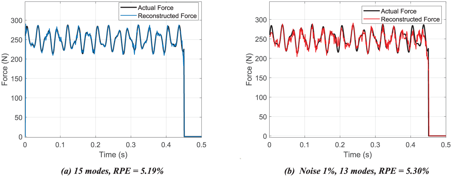
Optimal modes for force reconstruction with a noise level of 1%. (a) Rigid supports case, (b) elastic supports case.

Optimal modes for force reconstruction with a noise levels of 3%. (a) Rigid supports case, (b) elastic supports case.

Optimal modes for force reconstruction with a noise levels of 5%. (a) Rigid supports case, (b) elastic supports case.
Effect of sensor location analysis
In this test, we examine the effect of the position of the sensor on the regularization of the moving load in the two beam cases. Applying the same moving force and taking the first 15 modes for the rigid supports case and 13 modes for the elastic support case, we vary the location of the
The two graphs presented, corresponding, respectively, to the case of rigid supports (Figure 11(a)) and the case of elastic supports (Figure 11(b)), illustrate the evolution of relative errors (RPE (%)) as a function of the normalized sensor position

Evolution of RPE as a function of the sensor position parameter. (a) Rigid supports case, (b) elastic supports case.
Effect of number of measuring points
The number of measurement points is selected in turn as follows: 1, 2, 3, and 4, respectively. The measurement points are evenly distributed along the beam. The following Table 4 presents the relative errors based on the chosen measurement points for each noise level.
The relative error values for each noise level at different measurement points for the two types of supports.
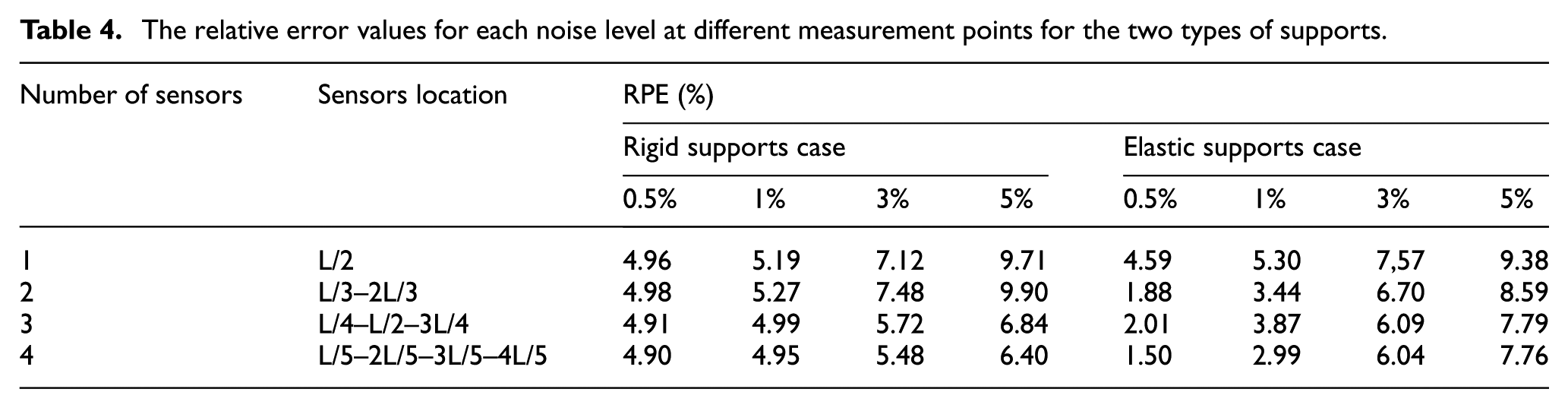
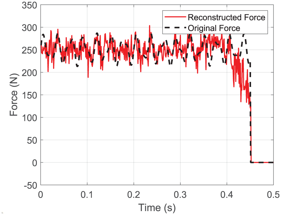
The results show that as the number of measurements increases, the relative error (RPE) decreases. Therefore, we conclude that adding sensors significantly improves accuracy, as with four measurement points the error stabilizes, even in the presence of noise, which indicates the importance of adequate coverage to improve identification for both cases of supports. Figures 12 to 15 show the optimal results for identifying the moving load with four measurement points for each type of noise for both cases of supports. As we can see, there is a significant improvement in the quality of identification when compared to the results obtained in Figures 7 to 10, which correspond to a single measurement point.

Optimal number of measuring points for force reconstruction with a noise levels of 0.5%. (a) Rigid supports case, (b) elastic supports case.

Optimal number of measuring points for force reconstruction with a noise levels of 1%. (a) Rigid supports case, (b) elastic supports case.

Optimal number of measuring points for force reconstruction with a noise levels of 3%. (a) Rigid supports case, (b) elastic supports case.

Optimal number of measuring points for force reconstruction with a noise levels of 5%. (a) Rigid supports case, (b) elastic supports case.
The results shown in the figures above illustrate the effect of the number of sensors on the quality of the reconstruction of the impact force history, which takes the form of a moving force. The stability ensured by using four sensors at a time is due to the quality of the measurements and their coverage of the entire beam. Additionally, when the noise level exceeds 3%, the quality of the reconstruction begins to deteriorate, especially in the case of an elastic support.
Influence of excitation frequency
In this section, we aim to study the effect of the excitation frequency of the moving force on the regularization of the moving load, applied over the entire length of the beam. The sensor is located in the middle of the beam (

Where
Figure 16 shows the variation of the RPE as a function of the excitation frequency. The results show that, for the rigid case, the variation of relative errors as a function of excitation frequencies is generally stable (the variations are small), but at the frequency

Evolution of the RPE as a function of the excitation frequency. (a) Rigid supports case, (b) elastic supports case.
Effect of spring stiffness
We have discussed the boundary conditions for both a rigid support and an elastic support with a moderate stiffness of 1000 N/m. Next, we attempted to reduce the stiffness to a value of 1 N/m, which is close to a free edge in reality. In this context, we aim to demonstrate that, for an acceptable reconstruction, the stiffness must be greater than a certain threshold. It should be noted that for very low stiffness values, the reconstruction quality is poor, especially when the signal is noisy and the noise level is low. Figure 17 shows the evolution of the impact force as a function of time for a noise level of 0.5%.
Reconstruction of impact force as a function of time with a noise level of 0.5%.
To illustrate the overall effect of the stiffness of the elastic support on the quality of impact force identification, the relative error shown in Figure 18 reaches its maximum for low stiffness, particularly for an elastic support with a stiffness of 1 N/m. This error begins to decrease as the stiffness increases and stabilizes once the stiffness becomes large enough for the support to behave as rigid.

Evolution of the RPE as a function of stiffness with a noise level varied from 0.5% to 5%.
Conclusions
The identification problem of impact force is an essential approach for monitoring the health of structures. Generally, this inverse problem is considered ill-posed, which has led to the use of regularization methods to stabilize the measurements obtained during the inversion of the matrix system. In this context, the selected regularization methods Tikhonov, TGSVD, and Tikhonov-SVD were tested against several parameters in order to select the most suitable one. First, sensitivity to noise was analyzed. Noise, as a disturbing factor, is crucial for testing the robustness of the regularization methods. Compared to the results obtained with standard Tikhonov and TGSVD, the Tikhonov-SVD regularization proves to be more applicable to moving load identification problems. An optimization of the
Footnotes
Handling Editor: Marek Chalecki
Funding
The authors received no financial support for the research, authorship, and/or publication of this article.
Declaration of conflicting interests
The authors declared no potential conflicts of interest with respect to the research, authorship, and/or publication of this article.