Sage Journals: Discover world-class research

Abstract

The pump-turbine is a key component in pumped-storage power stations, operating under complex conditions. RANS (Reynolds-Averaged Navier-Stokes) is commonly used for numerical simulations, but the differences among various RANS models under different operating conditions have not been systematically studied. This study aims to develop an energy loss method as a numerical model to quantitatively investigate pump-turbines using the most suitable turbulence model. The applicability of six turbulence models for numerical simulations of pump modes and turbine modes was comprehensively compared. Results show that the Realizable k-ε model performs best in pump mode due to its minimal overall error, while the SST k-ω model is preferable for turbine mode analysis. The SST k-ω model provides the most accurate prediction of shaft power across various operating conditions. Additionally, a new methodology for analyzing energy losses in pump-turbines was introduced, revealing significant energy loss in the guide vane section in pump mode, linked to uneven flow velocities. In turbine mode, considerable energy loss occurs in the runner area, associated with high-speed regions between blades. These findings offer valuable insights for improving the accuracy of numerical studies of pump-turbines.

Keywords

turbulence models energy loss pump-turbines

Introduction

The reliability and stability of pump-turbines, as key components of pumped storage power stations, are crucial for the stability of power systems and the safety of plant facilities. In order to balance the grid load and achieve functions such as peak shaving, frequency regulation, and load balancing, pump-turbines need to switch frequently between pump and turbine modes.¹ However, these frequent transitions and load changes can lead to deterioration of the flow characteristics inside the units, resulting in coupled vibrations. In severe cases, this may cause incidents such as oscillations,^2,3 efficiency decreases,⁴ and shutdowns.⁵ Studying the changes in flow patterns and energy loss in the pump turbine can help identify solutions to these issues and has received much attention in recent years.

CFD technology, with advantages such as high computational efficiency and independence from experimental model limitations, has become a powerful tool for investigating the complicated flow patterns in pump-turbines. There are mainly three numerical simulation methods for turbulent flow: DNS (Direct Numerical Simulation, DNS), LES (Large Eddy Simulation, LES), and RANS (Reynolds-Averaged Navier-Stokes, RANS). DNS is a method that directly uses the instantaneous Navier-Stokes equations to calculate turbulence without simplifications or approximations, theoretically providing relatively accurate results. For instance, Pirozzoli et al.⁶ conducted direct numerical simulations of turbulent flow in a smooth, straight circular pipe and discovered that the peak of scalar variance in the buffer layer grows logarithmically, in good accordance with Townsend’s attached-eddy hypothesis. However, resolving the detailed spatial structures and rapid temporal variations in turbulent flows at high Reynolds numbers requires extremely small time and spatial steps, which poses significant computational challenges. Popov et al.⁷ conducted a direct numerical simulation study of the turbulent flow in a realistic scale reactor involute, which required computational costs amounting to millions of CPU hours. As a result, DNS is currently impractical in applications such as pump-turbines. Secondly, LES directly simulates the large-scale eddies in turbulent flows using the instantaneous Navier-Stokes equations and employs sub-grid scale models to approximate smaller-scale eddies. Fu et al.⁸ based on LES methods simulated a load rejection process of a pump-turbine model. Compared to the experiments, the simulation deviation in rotational speed was less than 5%, and the local maximum deviation of the fluctuating pressure did not exceed 30%. However, the computational requirements of LES are still relatively high, making large-scale computations difficult to conduct in engineering. In the numerical simulation of turbulent flow in pump-turbines, the most commonly used method is RANS. Many researchers have used various turbulence models under RANS to study the flow characteristics inside pump-turbines. Zhang et al.^9,10 used SST k-ω to study the pressure pulsation of the runner in different operating modes of the pump-turbine, and the results were consistent with the experiments. Liu et al.¹¹ studied the hump characteristics in the pump modes of pump-turbine based on SST k-ω, and found that hump characteristic might be related to the cavity flow. Yu et al.¹² applied the entropy production of turbine operating modes in a pump-turbine model based on Standard k-ε model, and the results were in good agreement with experimental results. Li et al.¹³ conducted three-dimensional transient numerical simulations of different operating conditions of pump-turbines based on the SST k-ω model, studying the transient process of the hump unstable region, and found that strength and scope of vortex groups will change with discharge reduction. Liang et al.¹⁴ compared four turbulence models (Standard k-ε, RNG k-ε, Standard k-ω, and SST k-ω) for unsteady simulation of the pump-turbine in pump mode and found that the predicted heads with the four turbulence models were close under the optimal operating condition and large flow rate condition. Yu et al.¹² conducted numerical simulations of a pump-turbine using the traditional k-ε model and evaluated energy losses using entropy production theory, with results consistent with experimental data. Based on the RNG k-ε model, Zuo et al.¹⁵ investigated pressure fluctuations caused by inter-blade vortices, with the numerical results aligned well with experimental measurements. Qin et al.¹⁶ studied the relationship between energy loss and vorticity in the flow field of a pump-turbine based on the SST k-ω model, achieving good agreement with the experimental results. Pavesi et al.¹⁷ used a DES-based Realizable k-ε model to conduct a transient study on the variable speed process of a pump-turbine, achieving satisfactory simulation results. Pu et al.¹⁸ conducted a CFD-DEM study on the solid-liquid two-phase flow mechanism in centrifugal pumps, with the turbulence model used in the CFD simulation being the Realizable k-ε model. Wang et al.¹⁹ investigated the flow instability and vortex evolution inside a three-twisted-blade pump using a DDES-based SST k-ω model, also obtaining good simulation results. Additionally, Kim et al.²⁰ conducted numerical simulations on a pump turbine using the RSM model and performed multi-objective optimization of the hydraulic performance of the pump turbine based on the numerical simulation results. Li et al.²¹ studied the hydraulic performance under different rotational speeds in turbine mode based on the numerical simulation results using the standard k-ε model, and the results indicate that it is recommended to operate above the rated speed. Liu et al.²² used the v²-f model based on the Standard k-ε model calculating the transient processes under off-design conditions such as load rejection and pump unloaded state in turbines by this model, the changes in internal flow fields and external characteristics of the turbine were revealed. Zhang et al.^23,24 studied the internal flow characteristics of a reversible pump-turbine using the SST k-ω model and analyzed the relationship between vortices and blade pressure fluctuations. Liu et al.²⁵ conducted a numerical simulation of the shutdown process of a centrifugal pump based on the Realizable k-ε model, and the numerical simulation results agreed well with the theoretical analysis results.

Compared to the increasing number of studies on the flow characteristics in pump-turbines, few researches have been on the applicability of turbulence models in numerical simulations in different operating modes. There is virtually no systematic analysis of the accuracy of different turbulence models under various operating modes of the prototype hydraulic pump turbine. Therefore, there is a need for a more unified approach to studying the suitability of turbulence models and computational methods for simulating turbulent flow in energy storage units. On the other hand, pump-turbine play an important role in energy conversion in pumped storage power stations, effectively assessing the hydraulic losses during the operation of pump-turbines is crucial for studying the relationship between unsteady flow characteristics and hydraulic losses. What is more, after determining the appropriate turbulence model for the simulating of complicated flow in the pump-turbine, it is also necessary to establish an alternative energy loss analysis model based on the flow field results. Currently, in the field of hydraulic machinery, there are two main categories of methods for quantitatively calculating hydraulic losses in rotating fluid machinery. One category is based on entropy theory, such as the entropy production method and the entropy dissipation method, the other is based on the mean kinetic energy equation. Yuan et al.²⁶ used the entropy production method to investigate the energy losses of low specific speed centrifugal pumps under two different operating modes. Kan et al.²⁷ studied the energy losses involved in the process of axial pumps transitioning from pump mode to turbine mode, also based on the entropy production method. Lin et al.²⁸ used the entropy dissipation method to analyze energy losses in the numerical simulation results of a pump as turbine based on the SST model, and found that this method has certain advantages in the rotating domain. Qin et al.²⁹ proposed the local hydraulic loss rate method based on the average kinetic energy equation and applied it to the assessment of hydraulic losses in pump-turbine operating conditions, concluding that compared to the entropy theory, the average kinetic energy equation can better describe the distribution and evolution of hydraulic losses in the bladeless regions between the draft tube outlet, the runner inlet, and the guide vane exit under partial load operating points. However, most existing studies primarily focus on model pump turbines. Analyzing the energy losses of prototype pump turbines in actual pumped-storage power station operations is more closely related to real-world conditions and has greater reference significance in relevant engineering fields.

The purpose of this study is to address this by selecting commonly used turbulence models (Standard k-ε, RNG k-ε, Realizable k-ε, Standard k-ω, SST k-ω, and RSM models) to conduct three-dimensional numerical simulations of a pump-turbines with two guide-vane angles in engineering (22° and 37°) under two operating conditions (pumping and generating) and presents an energy loss model based on fluid computational domain integration. The structure of this paper is arranged as follows: The turbulence models compared, CFD settings, and the proposed energy loss model were introduced in Section “Simulation method.” Subsequently, a comprehensive analysis of the applicability of different turbulence models under various operating conditions based on experimental parameters was conducted. Next, the energy loss distribution and internal flow characteristics of the pump turbine under different operating conditions were analyzed, based on the simulation results with the least error. Finally, the conclusion was drawn.

Simulation method

Turbulent models

RANS is a method for solving the time-averaged Reynolds equations. The core idea is to use a certain model to express the transient fluctuations of momentum in the time-averaged equations, and then solve the time-averaged equations. The Reynolds-averaged continuity and momentum equations are as follows:

\frac{\partial ρ}{\partial t} + \frac{\partial ρ {\bar{u}}_{i}}{\partial x_{i}} = 0

(1)

\frac{\partial (ρ {\bar{u}}_{i})}{\partial t} + \frac{\partial (ρ {\bar{u}}_{i} {\bar{u}}_{j})}{\partial x_{j}} = - \frac{\partial p}{\partial x_{i}} + \frac{\partial}{\partial x_{j}} (μ \frac{\partial {\bar{u}}_{i}}{\partial x_{j}} - - ρ \bar{{u'}_{i} {u'}_{j}}) + F_{i}

(2)

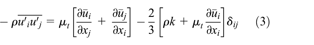
There are typically two types of turbulent models used in solving the time-averaged N-S equations: Reynolds stress model (RSM) and eddy viscosity model (EVM). The former constructs the Reynolds stress equations and solves them simultaneously with other governing equations, while the latter, based on the Boussinesq assumption, relates the Reynolds stress terms to the turbulent eddy viscosity μ_t. Below is a brief introduction to the turbulent models adopted in this paper.

The eddy viscosity assumption posits that the Reynolds stress correlated with turbulent velocity fluctuations can be analogized to the turbulent viscosity μ_t expressed as the gradient of the time-averaged velocity in turbulence, namely

- ρ \bar{{u'}_{i} {u'}_{j}} = μ_{t} [\frac{\partial {\bar{u}}_{i}}{\partial x_{j}} + \frac{\partial {\bar{u}}_{j}}{\partial x_{i}}] - \frac{2}{3} [ρ k + μ_{t} \frac{\partial {\bar{u}}_{i}}{\partial x_{i}}] δ_{ij}

(3)

In the equation above, ${\bar{u}}_{i}$ represents the time-averaged velocity, δ_ij is the Kronecker delta symbol, k is the turbulent kinetic energy, and the expression is

k = \frac{1}{2} ({\bar{u'}}^{2} + {\bar{v'}}^{2} + {\bar{w'}}^{2})

(4)

where $\bar{u'}$ , $\bar{v'}$ , and $\bar{w'}$ denote the average values of the components of turbulent velocity in the three directions. Therefore, the key to the eddy viscosity model lies in determining the turbulent viscosity μ_t. Currently, commonly used eddy viscosity models include: Standard k-ε, RNG k-ε, Realizable k-ε, Standard k-ω, and SST k-ω.

(1) Standard k-ε model: Based on the one-equation model, this model introduces a new equation for turbulent dissipation rate ε. The turbulent viscosity μ_t is expressed as a function of turbulent kinetic energy k and turbulent dissipation rate ε, where $C_{μ}$ is an empirical constant, and ρ is density,

μ_{t} = ρ C_{μ} \frac{k^{2}}{ε}

(5)

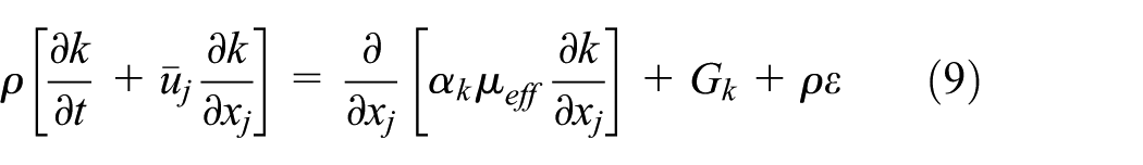
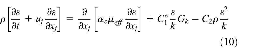
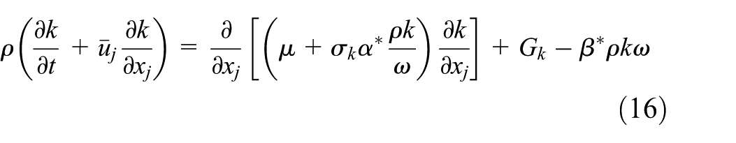
The turbulent kinetic energy equation and the turbulent dissipation rate equation are as follows

ρ (\frac{\partial k}{\partial t} + {\bar{u}}_{j} \frac{\partial k}{\partial x_{j}}) = \frac{\partial}{\partial x_{j}} [(μ + \frac{μ_{t}}{σ_{k}}) \frac{\partial k}{\partial x_{j}}] + G_{k} - ρ ε

(6)

ρ (\frac{\partial ε}{\partial t} + {\bar{u}}_{j} \frac{\partial ε}{\partial x_{j}}) = \frac{\partial}{\partial x_{j}} [(μ + \frac{μ_{t}}{σ_{ε}}) \frac{\partial ε}{\partial x_{j}}] + \frac{C_{1} ε}{k} G_{k} - C_{2} ρ \frac{ε^{2}}{k}

(7)

G_{k} = μ_{t} (\frac{\partial u_{i}}{\partial x_{j}} + \frac{\partial u_{j}}{\partial x_{i}}) \frac{\partial u_{i}}{\partial x_{j}}

(8)

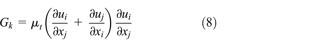
where G_k represents the production term of turbulent kinetic energy k making it demonstrate good numerical capturing performance for fully developed turbulence such as the turbulence inside pump-turbines, C₁ and C₂ are empirical constants, σ_k and σ_ε are the Prandtl numbers corresponding to k and ε, respectively. In the standard k-ε model, based on the recommendations of Launder et al. and experimental validation, the model parameters are suggested to be: C₁ = 1.44, C₂ = 1.92, C_μ = 0.09, σ_k = 1.0, and σ_ε = 1.3. The Standard k-ε model is developed for high-Reynolds-number turbulent flows with fully developed turbulence. It assumes that the turbulent viscosity μ_t is an isotropic scalar. When applied to flows involving strong rotation, curved wall surfaces, or curved streamlines, it can introduce certain inaccuracies.

(2) RNG k-ε model: Turbulence flow is considered as a transport process driven by random forces in this model. The small-scale motions are ignored through spectral analysis and their effects are incorporated into eddy viscosity, so that obtaining the transport process at the required scales. The k equation and ε equation of RNG k-ε model are similar to Standard k-ε model, but the turbulent viscosity is modified, considering the situations of rotation and rotational flow in the mean flow. The turbulent kinetic energy equation and the turbulent dissipation rate equation are present

ρ [\frac{\partial k}{\partial t} + {\bar{u}}_{j} \frac{\partial k}{\partial x_{j}}] = \frac{\partial}{\partial x_{j}} [α_{k} μ_{eff} \frac{\partial k}{\partial x_{j}}] + G_{k} + ρ ε

(9)

ρ [\frac{\partial ε}{\partial t} + {\bar{u}}_{j} \frac{\partial ε}{\partial x_{j}}] = \frac{\partial}{\partial x_{j}} [α_{ε} μ_{eff} \frac{\partial ε}{\partial x_{j}}] + C_{1}^{*} \frac{ε}{k} G_{k} - C_{2} ρ \frac{ε^{2}}{k}

(10)

C_{1}^{*} = C_{1} - \frac{η (1 - \frac{η}{η_{0}})}{1 + β η^{3}}, η = \sqrt{(2 E_{ij} \cdot E_{ij})} \frac{k}{ε}, E_{ij} = \frac{1}{2} (\frac{\partial u_{i}}{\partial x_{j}} + \frac{\partial u_{j}}{\partial x_{i}})

(11)

where μ_eff is the modified turbulent viscosity based on the RNG (Renormalization Group, RNG) theory, and α_k and α_ε are the reciprocals of the Prandtl numbers for k and ε, respectively. The RNG k-ε model is theoretically better suited for strongly swirling flows.

(3) Realizable k-ε model: To correct possible negative normal stress in the Standard k-ε model computations and to make the flow comply with physical laws, certain mathematical constraints need to be applied to the normal stress. Realizable k-ε model has two major differences from the previous two models. Firstly, this model considers the coefficient $C_{μ}$ in the turbulent viscosity calculation equation to be variable and related to the strain rate. The second difference is the modification made to the ε equation. The ε equation and the expressions for the $C_{μ}$ considered by this model are respectively as follows

ρ (\frac{\partial ε}{\partial t} + {\bar{u}}_{j} \frac{\partial ε}{\partial x_{j}}) = \frac{\partial}{\partial x_{j}} [(μ + \frac{μ_{t}}{σ_{ε}}) \frac{\partial ε}{\partial x_{j}}] + ρ C_{1} E ε - ρ C_{2} \frac{ε^{2}}{k + \sqrt{υ ε}}

(12)

C_{μ} = \frac{1}{A_{0} + A_{S} U^{*} \frac{k}{ε}}

(13)

the A₀ is generally taken as 4, A_S, U^*, and E are related to the turbulent time-averaged velocity gradient, $υ$ is dynamic viscosity. The specific flow cases or phenomena where the Realizable k-ε model demonstrates superiority over the RNG k-ε model have not yet been clearly identified.

(4) Standard k-ω model: This model, consisting of two equations, the k-equation and the ω-equation, is different from the Standard k-ε model in that it accurately predicts boundary layer flow with adverse pressure gradients. Additionally, Standard k-ω model considers low Reynolds numbers, compressibility, and the propagation of shear flows in its calculations, making it well-suited for calculating the low Reynolds number flow near the wall. In the Standard k-ω model, the turbulent dissipation rate ω is defined as

ω = \frac{ε}{C_{u} k}

(14)

The formula for turbulent viscosity, μ_t is as follows

μ_{t} = α^{*} \frac{ρ k}{\hat{ω}}

(15)

The variables α* and $\hat{ω}$ are determined by another formula. The equations for turbulent kinetic energy k and specific rate of turbulent dissipation ω are given

ρ (\frac{\partial k}{\partial t} + {\bar{u}}_{j} \frac{\partial k}{\partial x_{j}}) = \frac{\partial}{\partial x_{j}} [(μ + σ_{k} α^{*} \frac{ρ k}{ω}) \frac{\partial k}{\partial x_{j}}] + G_{k} - β^{*} ρ k ω

(16)

\begin{matrix} ρ (\frac{\partial ω}{\partial t} + {\bar{u}}_{j} \frac{\partial ω}{\partial x_{j}}) = \frac{\partial}{\partial x_{j}} [(μ + σ_{ω} α^{*} \frac{ρ k}{ω}) \frac{\partial ω}{\partial x_{j}}] \\ + γ \frac{ω}{k} G_{k} - β ρ ω^{2} + \frac{ρ σ_{d}}{ω} \frac{\partial k}{\partial x_{j}} \frac{\partial ω}{\partial x_{j}} \end{matrix}

(17)

where other model parameters such as β*, σ_ω, β, σ_d, γ, etc. are determined by separate formulas. There is a notable issue with the Standard k-ω model: the model is highly sensitive to the free-stream ω value. When the specified ω at the inlet changes, the simulation results can vary significantly.

(5) SST k-ω model: The model applies the standard k-ω model inside the boundary layer using a blending function and transforms the k-ε model for application in the fully turbulent developed region outside the boundary layer. The turbulent viscosity μ_t is further constrained as

μ_{t} = \frac{ρ a_{1} k}{max (a_{1} ω, Ω F)}

(18)

where typically a₁ is taken as 0.31, and F is a blending function. The k-equation and ω-equation of this model are

ρ (\frac{\partial k}{\partial t} + {\bar{u}}_{j} \frac{\partial k}{\partial x_{j}}) = \frac{\partial}{\partial x_{j}} [(μ + σ_{k} μ_{t}) \frac{\partial k}{\partial x_{j}}] + G_{k} - β^{*} ρ k ω

(19)

\begin{matrix} ρ (\frac{\partial ω}{\partial t} + {\bar{u}}_{j} \frac{\partial ω}{\partial x_{j}}) = \frac{\partial}{\partial x_{j}} [(μ + σ_{ω} μ_{t}) \frac{\partial ω}{\partial x_{j}}] \\ + \frac{γ}{μ_{t}} G_{k} - β ρ ω^{2} + 2 (1 - F) \frac{ρ σ_{d}}{ω} \frac{\partial k}{\partial x_{j}} \frac{\partial ω}{\partial x_{j}} \end{matrix}

(20)

The main feature of the SST k-ω model is its ability to effectively predict the onset point of flow separation within the boundary layer and the extent of the separation region under adverse pressure gradient conditions.

(6) Reynolds Stress Model: Unlike the eddy viscosity models described above, the Reynolds Stress Model (RSM) directly formulates and solves differential equations for the turbulent fluctuation stress terms in the Reynolds equations. This model requires solving the transport equation for Reynolds stress

\begin{matrix} \frac{\partial \bar{{u'}_{i} {u'}_{j}}}{\partial t} + \frac{\partial {\bar{u}}_{k} \cdot \bar{{u'}_{i} {u'}_{j}}}{\partial x_{k}} = - (\bar{{u'}_{j} {u'}_{k}} \frac{\partial {\bar{u}}_{i}}{\partial x_{k}} + \bar{{u'}_{i} {u'}_{k}} \frac{\partial {\bar{u}}_{j}}{\partial x_{k}}) \\ - 2 υ \bar{\frac{\partial {u'}_{i}}{\partial x_{k}} \frac{\partial {u'}_{j}}{\partial x_{k}}} - \frac{1}{ρ} ({u'}_{i} \frac{\partial p'}{\partial x_{j}} + {u'}_{j} \frac{\partial p'}{\partial x_{i}}) - \frac{\bar{\partial {u'}_{i} {u'}_{j} {u'}_{k}}}{\partial x_{k}} \\ + υ \frac{\partial^{2} \bar{{u'}_{i} {u'}_{j}}}{\partial x_{k}^{2}} \end{matrix}

(21)

For general three-dimensional problems, RSM requires solving six Reynolds stress differential equations, resulting in high computational cost, slower calculation speeds, and higher demands on computer resources.

Physical model and operating conditions

This paper takes a pump-turbine in a Chinese pumped storage power station as the prototype, which includes five parts: spiral casing, stay vanes, guide vanes, runner, and draft tube. Using the 3D modeling software UG NX, a three-dimensional hydraulic model of the pump-turbine full flow passage was created, as shown in Figure 1. The runner diameter of the pump-turbine is 4692 mm, the rated speed is 333.33 rpm, the number of blades is 9, and the number of stay vanes and guide vanes is both 20 (Table 1).

Figure 1.

Hydraulic model of the pump-turbine.

Table 1.

Main geometric parameters of the pump-turbine.

Parameters	Runner diameter	Stay vanes number	Guide vanes number	Blades number	Rated speed
Value	4692 mm	20	20	9	333.33 rpm

The test value of the head in the turbine mode is 319.41 m, with a flow rate of 74.20 m³/s, a power of 215.66 MW, and a hydraulic efficiency of 92.80%. According to the efficiency test of the pump-turbine under pump operation, at a flow rate of 73.81 m³/s and 250.72 MW power input, the head in the pump mode is 323.07 m, with an efficiency of 93.26%. In this paper, six turbulent models were used to conduct numerical simulations of the pump-turbine with two guide vane angles in engineering (ϕ = 22° and ϕ = 37°) under two operating conditions (pumping and generating).

Grid partition and boundary conditions

Considering both computational resource consumption and solution accuracy, the structured grid was used to partition the simple structural component of the draft tube, while the unstructured grid was used to partition the complex structural components of the spiral casing, stay vanes, guide vanes, and runner in the ANSYS ICEM 2021 R1 platform. The grid quality for each part was required to be above 0.4. To obtain a grid-independent solution, local refinements were applied to complex flow areas such as the guide vane surfaces, runner blade tips and ends, and spiral casing to ensure the reliability of the flow field calculation. Grid refinements were also applied near the wall to accommodate wall functions, with the y⁺ values for the entire computational domain ranging from 30 to 300, and for the SST k-ω model, the y⁺ value is small than 5.

The grid convergence method based on Richardson extrapolation is a highly recognized approach for grid independence verification in CFD and is strongly recommended by the Journal of Fluids Engineering.³⁰ In this study, referencing relevant literature,^10,26 the grid independence was validated using head as the evaluation variable through the grid convergence method. Three different grids were constructed, labeled as N₁, N₂, and N₃, with grid sizes increasing from small to large. The grid counts are 17.89 million, 12.78 million, and 9.13 million, respectively. The specific indicators of grid convergence are shown in Table 2, where $ϕ_{1}$ , $ϕ_{2}$ , $ϕ_{3}$ represent the evaluation variable values obtained from each grid, p is the apparent order, $ϕ_{12}^{ext}$ and $ϕ_{32}^{ext}$ are Richardson extrapolated values, ${GCI}_{12}^{fine}$ and ${GCI}_{32}^{coarse}$ are the fine-grid convergence indices. It is generally considered that a grid convergence index below 5% indicates a reliable grid resolution. In this case, ${GCI}_{12}^{fine}$ and ${GCI}_{32}^{coarse}$ are 0.71% and 0.81%, respectively, demonstrating that all three grids achieved reliable numerical solutions. Additionally, as is shown in Figure 2, the N₁ and N₂ grids’ evaluation variable values are between the two Richardson extrapolation values. Considering both computational accuracy and cost, the N₂ grid scheme with 12.78 million grids was selected for further analysis, as demonstrated in Figure 3. The detailed grid partition information is presented in Table 3.

Table 2.

Grid independency analysis.

N₁ (×10⁶)	N₂ (×10⁶)	N₃ (×10⁶)	$ϕ_{1}$ (m)	$ϕ_{2}$ (m)	$ϕ_{3}$ (m)	p	$ϕ_{12}^{ext}$	$ϕ_{32}^{ext}$	${GCI}_{12}^{fine}$	${GCI}_{32}^{coarse}$
17.89	12.78	9.13	309.23	309.51	309.44 m	6.41	309.27 m	310.21 m	0.71%	0.81%

Figure 2.

Grid independency based on Richardson.

Figure 3.

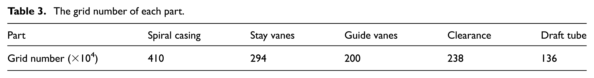
The grid partition of each part: (a) spiral casing, (b) stay vanes and guide vanes, (c) runner, and (d) draft tube.

Table 3.

The grid number of each part.

Part	Spiral casing	Stay vanes	Guide vanes	Clearance	Draft tube
Grid number (×10⁴)	410	294	200	238	136

In this paper, the governing equations are discretized through the finite volume method, and solved by the SIMPLEC algorithm. A high-order discretization scheme is applied to discretize the convective terms, and a second-order upwind scheme is adopted to discretize the diffusion terms.

One purpose of the present paper is to investigate the applicability of different turbulence models in the numerical simulation of pump-turbines, which conducted calculating under pump and turbine operating conditions at a rated speed of 333.33 rpm. In the pump mode, the draft tube was set as the inlet boundary with a flow rate inlet of Q = 73.81 m³/s, and water flowed into the vertical inlet surface. The inlet of the spiral casing was set as an outflow boundary. For the turbine operating condition, the inlet of the spiral casing was set as a pressure inlet with a pressure of 3,230,700 Pa, and the draft tube outlet condition was set as a flow-rate outlet with a flow rate of 74.20 m³/s. As to the runner section, we simulated the motion of the rotor component in Fluent using the multiple reference frame (MRF) method, where the fluid around the runner was set to a rotating reference frame with a rotational speed equal to the runner’s rotational speed. A rotating speed was set at the rated value of 333.33 rpm with the pump operating condition and the turbine operating condition rotating in opposite directions. The wall boundary conditions were applied to the draft tube, stay vanes, guide vanes, and turbine walls. The numerical simulations were performed on the Ansys Fluent 2022 software (Table 4).

Table 4.

Boundary conditions setup.

Mode	Inlet boundary			Outlet boundary			Rated speed
	Part	Set	Values	Part	Set	Values	Values
Pump	Draft tube	Flow-rate	73.81 m³/s	Spiral casing	Outflow		333.33 rpm
	Part	Set	Values	Part	Set	Values	Values
Turbine	Spiral casing	Pressure	3,230,700 Pa	Draft tube	Flow-rate	74.20 m³/s	333.33 rpm

External characteristic and energy loss

Head, shaft power, and hydraulic efficiency are key parameters of pump-turbines, and detailed tests must be conducted in engineering applications. These three parameters can also reflect the calculating effectiveness of the turbulence model for flow to a certain extent. The head is correlated to the energy of the fluid at the input and output, as well as the energy losses generated by the flow. Shaft power is related to the pressure torque and viscous torque exerted on the runner by the flow. Hydraulic efficiency can comprehensively reflect the energy conversion efficiency of the pump turbine. Therefore, this paper compared the prediction results of head, shaft power, and hydraulic efficiency using different turbulence models with prototype parameters, and analyzed the applicability of different turbulence models. Then, the energy loss distribution was calculated based on the results of the best turbulence models under different operating conditions according to the model^31–33 presented by the author applied in other field, and the related flow patterns of pump-turbines under different operating conditions were analyzed.

During the operation of pumps and turbines, intense turbulent flow has formed within pump-turbines. The generation and dissipation of turbulence have been accompanied by the energy transfer and dissipation, resulting in the energy losses in the whole process. Based on the Navier-Stokes equation, the energy loss equation corresponding to turbulent flow can be derived. First, the average kinetic energy equation for incompressible flow can be obtained according to the Navier-Stokes equation

\begin{matrix} \frac{\partial}{\partial x_{j}} (\frac{\bar{P}}{ρ g} + Z + \frac{{\bar{u}}_{i}^{2}}{2 g}) g {\bar{u}}_{j} \\ = 2 υ \frac{\partial ({\bar{u}}_{i} {\bar{T}}_{ij})}{\partial x_{j}} - \frac{\partial ({\bar{u}}_{i} \bar{{u'}_{i} {u'}_{j}})}{\partial x_{j}} - 2 υ {\bar{T}}^{2}_{ij} + \bar{{u'}_{i} {u'}_{j}} {\bar{T}}_{ij} \end{matrix}

(22)

Combined the average kinetic energy equation over the computational domain with the difference in energy between the inlet and outlet,^23,24 finally, the energy loss $Δ E$ generated by the fluid in the computational domain was derived

\begin{matrix} Δ E = \underset{in}{\int \int} (\frac{\bar{P}}{ρ g} + Z + \frac{{\bar{u}}_{i}^{2}}{2 g}) g {\bar{u}}_{j} n_{j} dS - \underset{out}{\int \int} (\frac{\bar{P}}{ρ g} + Z + \frac{{\bar{u}}_{i}^{2}}{2 g}) g {\bar{u}}_{j} n_{j} dS \\ = - \underset{1}{\underset{in}{\int \int} 2 {\bar{u}}_{i} (υ + μ_{t}) {\bar{T}}_{ij} n_{j} dS} + \underset{2}{\underset{out}{\int \int} 2 {\bar{u}}_{i} (υ + μ_{t}) {\bar{T}}_{ij} n_{j} dS} \\ + \underset{3}{\underset{V}{\int \int \int} 2 υ {\bar{T}}_{ij} \cdot {\bar{T}}_{ij} dV} - \underset{4}{\underset{V}{\int \int \int} (\bar{{u'}_{i} {u'}_{j}}) {\bar{T}}_{ij} dV} + \underset{5}{\underset{V}{\int \int \int} 2 (μ_{t} {\bar{T}}_{ij}) {\bar{T}}_{ij} dV} \end{matrix}

(23)

where $υ$ is the dynamic viscosity of the fluid, n_j is the component of the outward normal, and ${\bar{T}}_{ij}$ is the strain rate tensor. Equation (22) is the formula used to calculate the energy loss in stationary components of a pump-turbine, such as guide vanes. And the energy loss in rotating machinery, such as a runner

\begin{matrix} Δ E = - \underset{1}{\underset{in}{\int \int} 2 ω_{i} r_{i} (υ + \frac{ρ w_{i} r_{i}^{2}}{υ} μ_{e}) {\bar{T}}_{ij} n_{j} dS} \\ + \underset{2}{\underset{out}{\int \int} (ω_{i} r (\bar{{u'}_{i} {u'}_{j}})) n_{j} dS} + \underset{3}{\underset{V}{\int \int \int} 2 υ {\bar{T}}_{ij} \cdot {\bar{T}}_{ij} dV} \\ - \underset{4}{\underset{V}{\int \int \int} (\bar{{u'}_{i} {u'}_{j}}) {\bar{T}}_{ij} dV} + \underset{5}{\underset{V}{\int \int \int} 2 (\frac{ρ w_{i} r_{i}^{2}}{υ} μ_{e} {\bar{T}}_{ij}) {\bar{T}}_{ij} dV} \end{matrix}

(24)

where $w_{i}$ represents the angular velocity, $r_{i}$ represents the radius of rotation, and $μ_{e}$ is the eddy viscosity coefficient. In the formula (23) and (24), Parts 1 and 2 represent the diffusion of average kinetic energy, where Part 1 represents the input energy of the calculation domain, therefore a minus sign is in front of it. Part 3 represents the dissipation of average kinetic energy, Parts 4 and 5 represent the regeneration of turbulent energy. Since Part 5 accounts for over 99% of the numerical calculation in pump-turbines, the focus is on calculating the average energy loss represented by this part.

Result and discussion

In this section, numerical results and calculations of prototype parameters were conducted for two different guide vane angles (ϕ = 22° and ϕ = 37°) under conditions of runner speed of 333.33 rpm using six turbulence models for both turbine and pump modes. The different test parameters under various operating conditions were compared and analyzed entirely with prototype parameters to assess the applicability of different turbulence models in numerical simulations of pump and turbine modes. Then, in each operating mode with different guide vanes angels, the simulation results that best agree with the prototype parameters, combined with the energy conservation equation, were used to calculate the distribution of energy losses and analyze the internal flow characteristics of pump-turbines.

Validation of the hydraulic head

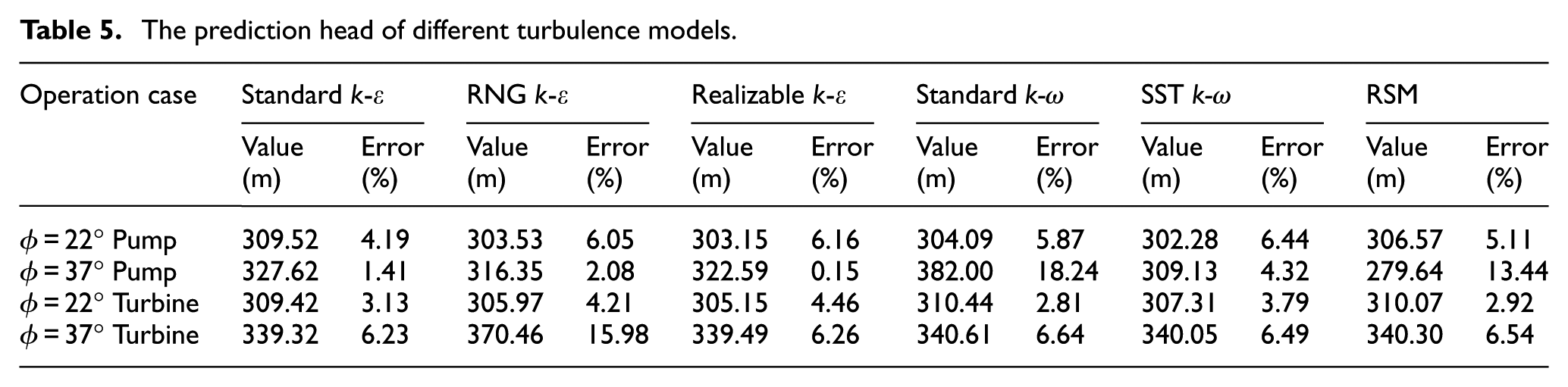
The calculation results of different turbulence models are summarized in Table 5, and the comparison of the predicted head for different operating conditions by different turbulence models is represented in Figure 4, where the left y-axis represents the head for the pump condition and the right y-axis indicates the net head for the turbine condition. Under test conditions the prototype pump condition has a head of 323.07 m (left y-axis, red dot line, Figure 4), while the net head for the turbine mode is 319.41 m (right y-axis, blue dot line, Figure 4). For the pump mode, the Realizable k-ε model had the most accurate prediction of head, especially with a prediction error of only 0.62% for a guide vane angle of 37°. For the turbine mode with a guide vane of 37°, the Standard k-ω model overestimates the head, with an error of 18.24%, while the RSM model underestimates the head, with an error of 13.44%. Compared to the other models, these two models have larger prediction errors for the head in turbine mode with a guide vane of 37°. All turbulence models underestimated the head in the pumping mode with a guide vane angle of 22°. For the turbine mode, except for the RNG k-ε model, which has a head prediction error exceeding 15% at a guide angle of 37°, the errors of the other turbulence models do not exceed 7%. All turbulence models underestimate the net head for turbine mode with a guide vane angle of 22° and overestimate the net head at a guide angle of 37°. For the turbine mode at a 37-degree opening angle, there is no significant difference in the prediction accuracy of the net head among the various turbulence models. However, for the turbine mode at a 22-degree opening angle, the Standard k-ω and RSM models perform slightly better than the other models.

Table 5.

The prediction head of different turbulence models.

Operation case	Standard k-ε		RNG k-ε		Realizable k-ε		Standard k-ω		SST k-ω		RSM
Operation case	Value (m)	Error (%)	Value (m)	Error (%)	Value (m)	Error (%)	Value (m)	Error (%)	Value (m)	Error (%)	Value (m)	Error (%)
ϕ = 22° Pump	309.52	4.19	303.53	6.05	303.15	6.16	304.09	5.87	302.28	6.44	306.57	5.11
ϕ = 37° Pump	327.62	1.41	316.35	2.08	322.59	0.15	382.00	18.24	309.13	4.32	279.64	13.44
ϕ = 22° Turbine	309.42	3.13	305.97	4.21	305.15	4.46	310.44	2.81	307.31	3.79	310.07	2.92
ϕ = 37° Turbine	339.32	6.23	370.46	15.98	339.49	6.26	340.61	6.64	340.05	6.49	340.30	6.54

Figure 4.

Comparison of head prediction results.

Validation of the shaft power

For a consistent flow rate and runner speed cases (73.81 m³/s and 333.33 rpm), the prototype pump-turbine in pump mode has a shaft power of 250.72 MW. At a turbine operating condition with a flow rate of 74.20 m²/s and a rotational speed of 333 rpm, the output shaft power of the runner is 215.66 MW. The calculated shaft power under different operating conditions by different turbulence models are given in Table 6, and Figure 5 compares the shaft power by different turbulence models. It can be observed that for the pump mode, most turbulence models overestimated the input shaft power for both pump modes with different guide vane angles. Only the RSM model underestimated the shaft power for the pump mode with a guide vane angle of 37°. All turbulence models had good predictions of shaft power close to the prototype parameter for the pump mode with a guide vane angle of 22°, but the prediction errors of shaft power for Standard k-ω model and RSM model were significantly larger than those of the other models. Overall, the SST k-ω model had the best predictive performance for shaft power in the pump condition, being closest to the prototype parameters, with prediction errors less than 2% for both guide vane angles in the pump mode. In the turbine mode, the predictions at a 22-degree opening angle by all turbulence models were underestimated, but all turbulence models overestimated the shaft power at a 37-degree opening angle. Under the turbine operating conditions, all models had similar prediction accuracy for shaft power, with the SST k-ω model performing slightly better than the other models, while the RNG k-ε model performed slightly worse. The SST k-ω model provided the best prediction performance for shaft power among all models. The SST k-ω model uses a blending function to apply the Standard k-ω model near the wall and the k-ε model in the turbulent flow region, while additionally considering the effect of turbulent shear stress on the construction of turbulent viscosity. These advantages allow it accurately simulate the viscous and pressure torques exerted by the fluid on the runner, resulting in more accurate predictions of shaft power.

Table 6.

The shaft power prediction results of different turbulence models.

Operation case	Standard k-ε		RNG k-ε		Realizable k-ε		Standard k-ω		SST k-ω		RSM
Operation case	Value (MV)	Error (%)	Value (MV)	Error (%)	Value (MV)	Error (%)	Value (MV)	Error (%)	Value (MV)	Error (%)	Value (MV)	Error (%)
ϕ = 22° Pump	256.87	2.45	257.43	2.68	255.13	1.76	256.26	2.21	254.65	1.57	256.19	2.18
ϕ = 37° Pump	267.26	6.60	259.78	3.61	263.43	5.07	301.97	20.44	255.21	1.79	230.26	8.16
ϕ = 22° Turbine	194.75	9.70	196.73	8.78	195.03	9.57	194.98	9.59	196.08	9.08	195.73	9.24
ϕ = 37° Turbine	222.11	2.99	227.70	5.58	221.93	2.97	222.22	3.04	222.43	3.14	223.20	3.50

Figure 5.

Comparison of shaft power prediction results.

Validation of the hydraulic efficiency

The prototype pump-turbine has a hydraulic efficiency of 92.80% and 93.26% in turbine mode and pump mode, respectively. The predicted hydraulic efficiency under different operating conditions by different turbulence models are listed in Table 7, and Figure 6 plots the predicted results by different turbulence models. As indicated in Figure 5 most turbulence models underestimated the hydraulic efficiency for both pump modes with different guide vane angles. For the pump mode with a guide vane angle of 22°, the predictions of hydraulic efficiency by various turbulence models were similar, with the Standard k-ε model having the smallest error at 5%; and for the pump mode with the larger guide vane angle (37°) the best prediction was by the Standard k-ω model with an error of only 0.12%. For turbine operating conditions, the Realizable k-ε model and the SST k-ω model showed a stable performance with relatively small errors in efficiency prediction at the two opening angles. For the turbine mode, the Realizable k-ε model showed an efficiency error of 4.79% at a 22-degree opening angle and 4.56% at a 37-degree opening angle. Similarly, the SST k-ω model exhibited an efficiency error of 4.94% at a 22-degree opening angle and 4.50% at a 37-degree opening angle. In summary, the Standard k-ω model has the best predictive performance for hydraulic efficiency in the pump mode, while the Realizable k-ε model the SST k-ω model outperforms other turbulence models in the turbine mode.

Table 7.

The hydraulic efficiency prediction results of different turbulence models.

Operation case	Standard k-ε		RNG k-ε		Realizable k-ε		Standard k-ω		SST k-ω		RSM
Operation case	Value (%)	Error (%)	Value (%)	Error (%)	Value (%)	Error (%)	Value (%)	Error (%)	Value (%)	Error (%)	Value (%)	Error (%)
ϕ = 22° Pump	88.94	5.00	87.03	6.68	87.70	5.96	87.59	6.08	87.62	6.05	88.33	5.29
ϕ = 37° Pump	90.48	2.98	89.89	3.62	90.39	3.08	93.37	0.12	89.40	4.14	89.64	3.88
ϕ = 22° Turbine	87.01	6.24	88.89	4.22	88.36	4.79	86.83	6.43	88.21	4.94	87.27	5.96
ϕ = 37° Turbine	88.68	4.44	83.27	10.27	88.57	4.56	88.39	4.75	88.62	4.50	88.86	4.24

Figure 6.

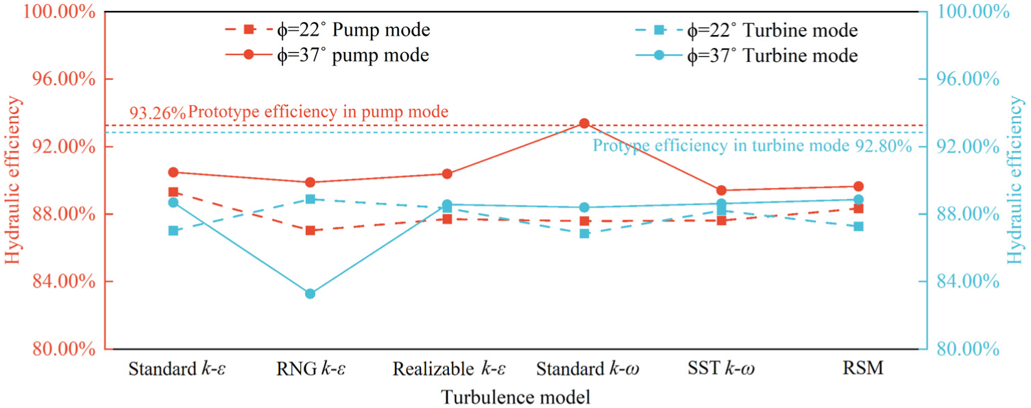
Comparison of hydraulic efficiency prediction results.

Applicability of turbulence models

The evaluation of the simulation performance of pump-turbines based on three parameters-head, shaft power, and hydraulic efficiency-focuses on different aspects. A comprehensive prediction error of these three parameters can provide a more complete and quantitative reflection of the applicability of different turbulence models for the pump and turbine modes of pump-turbines. Figures 7 and 8 summarize the cumulative prediction errors of different turbulence models for two guide vane angles (ϕ = 22° and ϕ = 37°) in pump-turbine for three parameters under pump and turbine mode, respectively. As detailed in Figure 6, the Realizable k-ε model had the smallest cumulative error under both guide vane angles for pump mode, with the cumulative errors of 13.88% and 8.30% for ϕ = 22° and ϕ = 37° cases, respectively. Therefore, the most suitable turbulence model for pump simulating mode is the Realizable k-ε model. In contrast, the Standard k-ω model and RSM model have a remarkably higher simulation errors for the ϕ = 37° pump mode than other turbulence models, from the perspective of error composition, these two models do not show a significant difference in predicting hydraulic efficiency compared to other models. However, the predicted values of shaft power and head demonstrate a similar trend. Therefore, the larger overall error is mainly due to the greater prediction error in the torque generated by the runner on the fluid under these conditions for both models. The potential reason for the largest shaft power prediction errors when using the Standard k-ω model is its high sensitivity to the inlet ω in the computational domain. Inappropriate values of the inlet turbulence intensity can significantly impact the results, especially in high Reynolds number regions far from the wall, where substantial errors may occur. Consequently, flow predictions in the runner section at higher Reynolds numbers are more prone to notable errors. For the turbine mode, as indicated in Figure 8, except for the RNG k-ε model, which had a noticeably higher cumulative error for the ϕ = 37° case, the rest of the turbulence models reported approximate cumulative errors. The predicted value of shaft power by the RNG k-ε model was close to the prototype test values under the consistent operating conditions, while the net head was higher than the test value, indicating that the model overestimated the energy loss. Although the RNG k-ε model is theoretically better suited for strongly swirling flows, under large-angle guide vane conditions in water turbines, the initial circulation imparted to the flow diminishes, and the rotational effects become less pronounced. This reduction in rotational influence leads to inaccuracies in turbulence viscosity modeling by the RNG k-ε model, resulting in larger flow prediction errors. For the turbine mode, the SST k-ω model has a lower cumulative error than other turbulence models, with cumulative errors of 17.81% and 14.11% for ϕ = 22° and ϕ = 37° cases, respectively, making it recommended for numerical simulation under turbine mode. In conclusion, the Realizable k-ε model and the SST k-ω model demonstrate a good predictive performance for all three evaluation parameters in various operating modes, surpassing other models in the numerical simulation of external flow characteristics within the pump-turbine.

Figure 7.

Cumulative errors in pump modes with different guide vanes angles.

Figure 8.

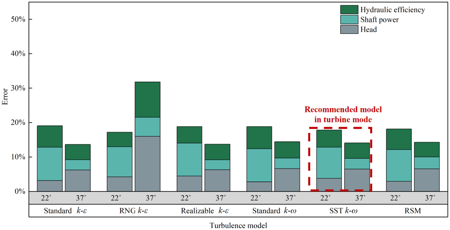
Cumulative errors in turbine modes with different guide vanes angles.

Distribution of the energy losses

As discussed above, it was found that the Realizable k-ε model has the smallest overall prediction error for the pump mode. By carrying out energy loss calculations based on the simulation results of the pump mode applying the Realizable k-ε model, it was discovered that there is a relatively high energy loss in the guide vane section of the pump-turbine. By comparing velocity contour and the energy loss distribution as displayed in Figure 9, it was observed that the energy loss in the guide vane section is mainly concentrated at the front end of the guide vane, which has a certain relationship with the flow velocity distribution at the guide vanes. The flow into the passage at the guide vane section is not uniform, with one side of the passage showing higher flow velocity than the other side. The results indicate that there is a correlation between flow velocity, non-uniformity velocity, and energy losses. The larger the non-uniformity velocity at both sides of the guide vanes, the greater the energy losses generated at the head and tail of the guide vanes. The high energy loss regions correspond roughly to the non-uniform velocity regions. The impact between the water flow exiting the runner and the guide vane may be the cause of this phenomenon. Under pump operating conditions, the guide vane front end obstructs the flow, resulting in significant energy loss.

Figure 9.

Energy loss and velocity contour of guide vanes in the pump mode (realizable k-ε model): (a) velocity contour and (b) energy loss.

Compared to the guide vane section, the high energy loss region in the runner section is much smaller under pump mode. Evidence for this is in Figure 10, the velocity contour and energy loss distribution in the runner section, at the high-speed region near the end of the runner, there is higher energy loss. Consistent with the observations by Yuan et al.²⁶ based on the entropy production method, the incident loss at the blade leading edge is a significant source of energy loss in the runner section in the pump mode.

Figure 10.

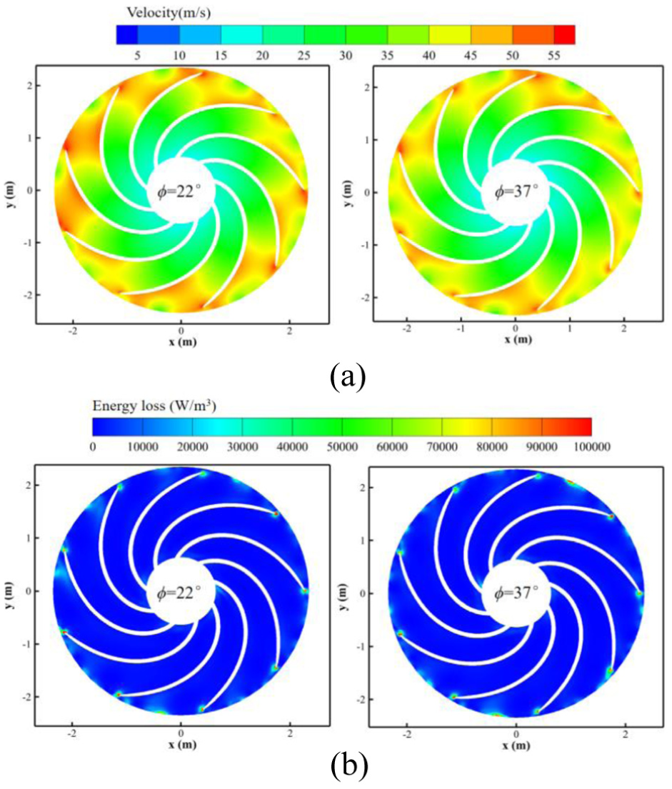
Energy loss and velocity contour of the runner section in the pump mode (realizable k-ε model): (a) velocity contour and (b) energy loss.

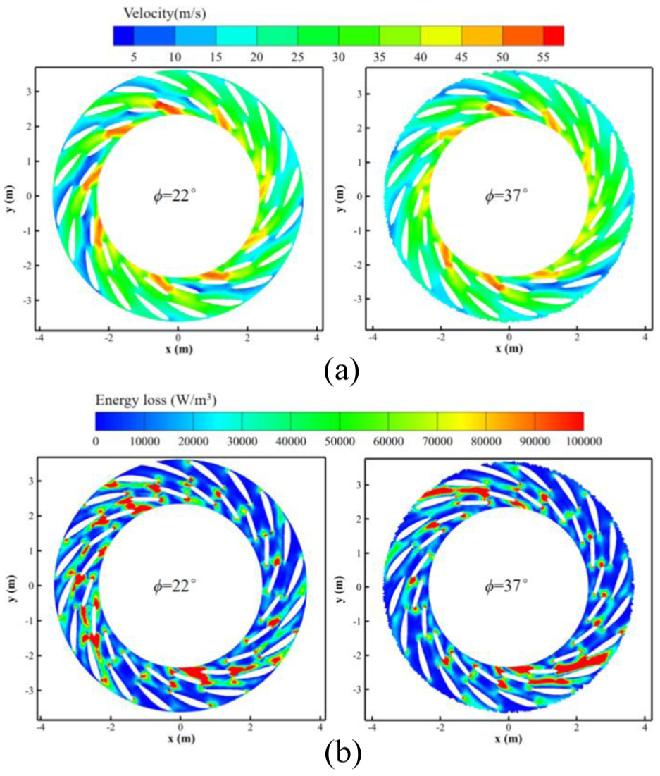
The SST k-ω model shows a strong applicability in the numerical simulation of turbine mode in pump-turbines. Through energy loss analysis based on the results of the turbine mode applying the SST k-ω model, it was found that there is a relatively high energy loss in the guide vanes section and the runner section. As illustrated in Figure 11, in the guides vanes section, the energy loss is greater near the tip of the guide vane close to the runner and the velocity in these regions are lower compared to the surrounding. Compared to the pump mode, the energy loss in the guide vane region is relatively small, with losses occurring only at the outlet, possibly influenced by the runner.

Figure 11.

Energy loss and velocity contour of guide vanes in the turbine mode (SST k-ω model): (a) velocity contour and (b) energy loss.

Figure 12 reveals the areas of partial high-speed flow between the backside of the runner blades and near the guide vane in the turbine mode. Comparatively, at different guide vane angles, the locations of the high-speed regions in the runner section are generally similar in the turbine mode, but the high-speed region at ϕ = 37° is closer to the backside of the blades. An analysis of the energy loss distribution indicated that when the high-speed region is positioned at the center of the passage between the blades, higher energy losses are incurred compared to when the high-speed region adheres to the backside of the blades. The area of high energy loss at ϕ = 37° is smaller than at ϕ = 22°. Therefore, the occurrence of the high-speed region may be related to the guide vane angle, and in the turbine mode, efforts should be made to ensure that the high-speed region adheres to the backside of the blades to minimize energy losses. Compared to Yuan et al.’s²⁶ study on turbine mode, the region of concentrated energy loss is also at the blade leading edge. However, in this paper, the energy loss is concentrated in the gap between the blade leading edges, while in Yuan’s research, the region is closer to the blade leading edge. Since Yuan’s study used a centrifugal pump model without guide vanes, whereas actual water pump turbines have guide vanes, the findings of this paper may be more representative of real-world conditions.

Figure 12.

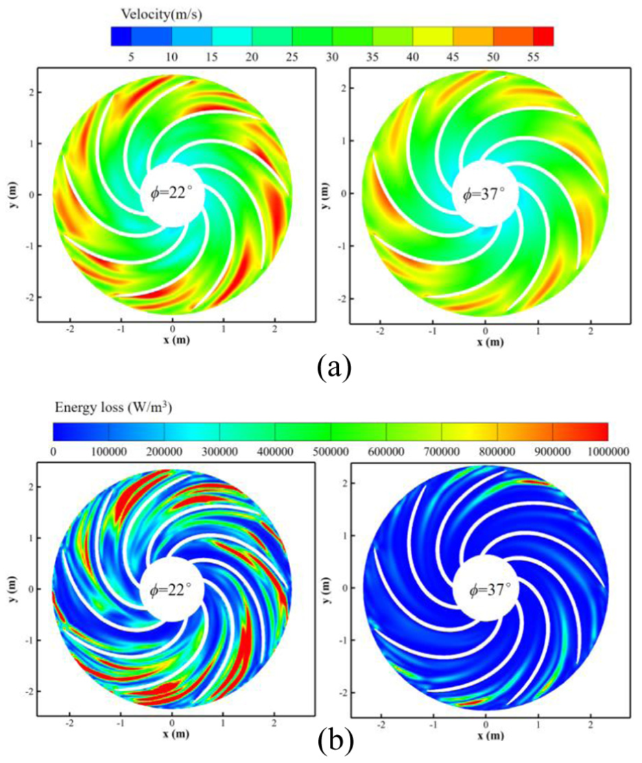
Energy loss and velocity contour of the runner section in the turbine mode (SST k-ω model): (a) velocity contour and (b) energy loss.

Conclusions

This study evaluated the performance of various turbulence models in numerical simulations of pump-turbine flow under pump and turbine conditions, focusing on head, shaft power, and hydraulic efficiency and analyzed the relationship between energy losses and flow characteristics. The conclusions are summarized as follows.

The Realizable k-ε and SST k-ω models demonstrated superior predictive accuracy across all parameters, with the Realizable k-ε model performing best in pump mode and the SST k-ω model excelling in turbine mode.

The SST k-ω model provided the most accurate shaft power predictions, with errors of 1.57% and 1.79% in pump conditions at 22° and 37° openings, respectively, and errors of 9.08% and 3.14% in turbine conditions.

In pump mode, energy loss near the guide vane is primarily due to uneven flow velocities between channels, with larger velocity gradients causing greater losses at the head and tail sections. In turbine mode, high energy loss in the runner correlates with high-velocity regions between blades, increasing when these regions are located between the blades.

These insights contribute to the understanding and optimization of pump-turbine performance and provide a reference for future numerical modeling efforts.

Footnotes

Appendix

Handling Editor: Minsuk Choi

ORCID iD

Zhiheng Wang

Ethical considerations

This article does not contain any studies with human participants or animals performed by any of the authors.

Consent to participate

Informed consent was obtained from all individual participants included in the study.

Author contributions

Conceptualization, Miao Guo, Xuelin Tang, and Xiaoqin Li; methodology, Miao Guo, Zhiheng Wang, and Xuelin Tang; validation, Zhiheng Wang, Yan Shen, Ruixiang Song; formal analysis, Zhiheng Wang, Yan Shen; investigation, Miao Guo, Xuelin Tang, and Xiaoqin Li; data curation, Yan Shen and Ruixiang Song; writing-original draft preparation, Miao Guo and Zhiheng Wang; writing-review and editing, Miao Guo and Zhiheng Wang; supervision, Xuelin Tang and Xiaoqin Li; project administration, Xuelin Tang and Xiaoqin Li; funding acquisition, Miao Guo.

Funding

The authors disclosed receipt of the following financial support for the research, authorship, and/or publication of this article: This research was funded by the National Natural Science Foundation of China (No. 52279084) and the Fundamental Research Funds for the Central Universities (No. 2024MS065).

Declaration of conflicting interests

The authors declared no potential conflicts of interest with respect to the research, authorship, and/or publication of this article.

Data availability statement

All relevant data are within the paper.

References

Mei

Pumped storage power generation technology. China Machine Press, 2000.

Liu

Zhao

Experimental study of the flow field of a high head model pump turbine based on PIV technique. J Hydrodynam 2021; 33(5): 1045–1055.

Zhang

Wang

, et al. Vibration control on coupled unit-plant structure of pumped storage power station during sudden load-up process. Mech Syst Signal Process 2024; 212: 111333.

Zhao

, et al. Water column separation under one-after-another load rejection in pumped storage station. Energy 2023; 278: 127809.

Kong

Liu

, et al. Pumped storage power stations in China: the past, the present, and the future. Renew Sustain Energy Rev 2017; 71: 720–731.

Pirozzoli

Romero

Fatica

, et al. DNS of passive scalars in turbulent pipe flow. J Fluid Mech 2022; 940: A45.

Popov

Mecham

Bolotnov

Direct numerical simulation of involute channel turbulence. J Fluids Eng 2024; 146: 081301.

Wang

, et al. Numerical simulation of the transient flow in a pump-turbine during load rejection process with special emphasis on hydraulic acoustic effect. Renew Energy 2020; 155: 1127–1138.

Zhang

Xiao

Zhu

, et al. Pressure pulsation reduction in the draft tube of pump turbine in turbine mode based on optimization design of runner blade trailing edge profile. J Energy Storage 2023; 59: 106541.

10.

Zhang

Fang

Tao

, et al. Investigation of energy loss patterns and pressure fluctuation spectrum for pump-turbine in the reverse pump mode. J Energy Storage 2023; 72: 108275.

11.

Liu

, et al. Numerical investigation of the hump characteristic of a pump–turbine based on an improved cavitation model. Comput Fluids 2012; 68: 105–111.

12.

, et al. Numerical study on the energy evaluation characteristics in a pump turbine based on the thermodynamic entropy theory. Renew Energy 2022; 195: 766–779.

13.

Wang

Xiang

, et al. Unsteady simulation and analysis for hump characteristics of a pump turbine model. Renew Energy 2015; 77: 32–42.

14.

Liang

Zhang

, et al. Study on pressure fluctuation and rotating stall characteristics in the vaneless space of a pump-turbine in pump mode. J Energy Storage 2024; 94: 112385.

15.

Zuo

Liu

, et al. Numerical analyses of pressure fluctuations induced by interblade vortices in a model Francis turbine. J Hydrodynam 2015; 27: 513–521.

16.

Qin

Wang

, et al. Investigation on the relationship between hydraulic loss and vortex evolution in pump mode of a pump-turbine. J Hydrodynam 2022; 34: 555–569.

17.

Pavesi

Cavazzini

Ardizzon

Numerical simulation of a pump–turbine transient load following process in pump mode. J Fluids Eng 2017; 140: 021114.

18.

, et al. Study on the particle dynamic characteristics in a centrifugal pump based on an improved computational fluid dynamics-discrete element model. Phys Fluids 2024; 36(12): 123331.

19.

Wang

Yang

Liang

, et al. Flow instability and vortex evolution in a three-twisted-blade pump using delayed detached eddy simulation. Phys Fluids 2025; 37: 025129.

20.

Kim

Suh

Choi

, et al. Simultaneous efficiency improvement of pump and turbine modes for a counter-rotating type pump-turbine. Adv Mech Eng 2016; 8: 112731.

21.

Zhang

Chen

, et al. Influence of rotational speed on performance of low specific speed hydraulic turbine in turbine mode. Adv Mech Eng 2022; 14: 1–13.

22.

Liu

Sun

, et al. Three-dimensional flow simulation of load rejection of a prototype pump-turbine. Eng Comput 2013; 29(4): 417–426.

23.

Zhang

Liu

, et al. Analysis of the vortices in the inner flow of reversible pump turbine with the new omega vortex identification method. J Hydrodynam 2018; 30: 463–469.

24.

Zhang

Liu

, et al. Numerical simulation of hydraulic force on the impeller of reversible pump turbines in generating mode. J Hydrodynam 2017; 29: 603–609.

25.

Liu

Zhou

Guo

, et al. 3-D CFD simulation of transients in multiple pump system with some pumps being stopped. J Hydrodynam 2021; 33: 583–592.

26.

Yuan

Zhang

Zhou

, et al. Hydraulic loss analysis in a pump-turbine with special emphasis on local rigid vortex and shear. Phys Fluids 2022; 34: 125101.

27.

Kan

Chen

, et al. Energy loss mechanisms of transition from pump mode to turbine mode of an axial-flow pump under bidirectional conditions. Energy 2022; 257: 124630.

28.

Lin

Zhu

, et al. Application of enstrophy dissipation to analyze energy loss in a centrifugal pump as turbine. Renew Energy 2021; 163: 41–55.

29.

Qin

Wang

, et al. Investigation on hydraulic loss component and distribution in hydraulic machinery: a case study of pump-turbine in pump mode. J Energy Storage 2022; 52: 104932.

30.

Celik

Ghia

Roache

, et al. Procedure for estimation and reporting of uncertainty due to discretization in CFD applications. J Fluids Eng 2008; 130(8): 078001.

31.

Guo

Wang

Song

, et al. Investigation on the hydraulic loss in the vertical inlet and outlet of a pumped storage power station. J Phys Conf Ser 2024; 28: 012079.

32.

Guo

Huang

Jiang

, et al. Research on the hydraulic loss in the side inlet and outlet of a pumped storage power station. J Phys Conf Ser 2024; 28: 012078.

33.

Guo

Liu

Tang

, et al. Evaluation of shaft forces in a vertical canned motor through local hydraulic loss analysis. Adv Mech Eng 2018; 10: 1–20.

Systematic analysis on the energy loss in pump-turbines

Abstract

Keywords

Introduction

Simulation method

Turbulent models

Physical model and operating conditions

Grid partition and boundary conditions

External characteristic and energy loss

Result and discussion

Validation of the hydraulic head

Validation of the shaft power

Validation of the hydraulic efficiency

Applicability of turbulence models

Distribution of the energy losses

Conclusions

Footnotes

Appendix

ORCID iD

Ethical considerations

Consent to participate

Author contributions

Funding

Declaration of conflicting interests

Data availability statement

References