Sage Journals: Discover world-class research

Abstract

To address issues of local optimization, slow convergence, and poor accuracy, this work introduces a time-optimal trajectory planning method using the Adaptive Gold Search algorithm (AGS). The method enhances algorithm diversity and escapes local optima through elite reverse strategy population initialization. It employs an adaptive nonlinear decreasing factor for a balance between linearity and nonlinearity, improving accuracy and convergence speed. The golden sinusoidal variation technique enhances global search capabilities and robustness in robot arm trajectory planning. Experimental results show that the AGS algorithm produces smooth joint angular displacement, acceleration, velocity, and jerk curves. It outperforms the GA, PSO, GOOSE, and GWO algorithms in time optimization by 13.31%, 13.61%, 5.34%, and 4.73%, respectively, effectively reducing trajectory planning time.

Keywords

industrial mechanical arm trajectory planning Adaptive Gold Search algorithm time optimization

Introduction

By defining the joint states of the end-effector, the robotic arm can move efficiently in accordance with the trajectory and precisely reach the target point, ensuring that the entire movement process takes the least amount of time, provided that the dynamic constraints and safety requirements of the system are met. This is known as time-optimal trajectory planning.

Intelligent optimization algorithms are applied to study and optimize various engineering problems because of their generality and parallel processing.^1–3 Meta-heuristic algorithms are typical of intelligent optimization algorithms because they can usually find the optimal solution of a problem in a relatively short time with high efficiency and flexibility. Metaheuristic algorithms are categorized into three types: evolutionary algorithms, swarm intelligence algorithms, and emergent metaheuristics. The proposal of evolutionary algorithms such as Genetic Algorithms (GA),⁴ Differential Evolution Algorithms (DE),⁵ and Tabu Search Algorithms (TS),⁶ pioneered the application of meta-heuristic algorithms in optimization. These algorithms solve problems like path planning⁷ and damage detection⁸ by simulating natural evolutionary processes. However, with the increasing complexity of practical engineering problems, evolutionary algorithms have shown limitations in addressing issues involving complex structures and forms. Subsequent research has consistently proposed Particle Swarm Optimization (PSO),⁹ Ant Colony Algorithm (ACA),¹⁰ Grey Wolf Optimizer (GWO),¹¹ Monkey Algorithm (MA),¹² and other swarm intelligence algorithms. These meta-heuristic algorithms are highly general and independent of the particular form and structure of the problem. In the study of PSO algorithms, it was discovered that swarm intelligent algorithms are easily prone to local optimization problems,¹³ while in the study of nonlinear optimization search problems, Jiang et al.¹⁴ discovered that the inability of swarm intelligent algorithms to adapt to complex nonlinear optimization search results in a decrease in algorithmic convergence accuracy. As a result, the traditional swarm intelligence algorithm finds it challenging to achieve optimal results for high-dimensional, nonlinear, multi-polar, objective function that cannot be deduced, and other complex global optimization problems. Spider Wasp Optimizer Algorithm (SWO),¹⁵ Nutcracker Optimization Algorithm (NOA),¹⁶ Zebra Optimization Algorithm (ZOA),¹⁷ and other emerging meta-heuristic algorithms proposed to solve the global optimization problem and convergence accuracy provides a new approach, but these algorithms lack adaptive adjustment mechanism and are sensitive to parameters. For this reason, researchers typically enhance the mechanism of meta-heuristic algorithms. Wu and Luo¹⁸ expand the search space by adding the enhanced mutation operator in the DE algorithm to the inertia weights of the PSO algorithm. Wu et al.¹⁹ enhance the PSO method by implementing the Gaussian mutation strategy and greedy strategy, which may guarantee that the process is difficult to fall into the local optimum by limiting the likelihood of particle mutation within a manageable range; Wang et al.²⁰ used the initialization strategy combining Fuch chaos mapping and optimized dyadic learning to generate a well-diversified population, which improves the global exploration ability of the Whale Optimization Algorithm (WOA) in dealing with high-dimensional optimization problems. However, the research of the above algorithms still suffers from the defects of poor convergence accuracy and slow convergence speed, and the advantages and disadvantages of the convergence effect directly affect the accuracy of the results of the search for optimization. For this purpose, Long et al.²¹ used a nonlinear control parameter convergence strategy to introduce random perturbations to enhance the robustness, which accelerated the convergence speed of the GWO algorithm; Bai and Liu²² combined the decomposition strategy with the Artificial Bee Colony Algorithm (ABC) to decompose the original multi-objective optimization into multiple single-objective optimization subproblems, which improved the convergence speed of the ABC algorithm; Liu et al.²³ combined local pheromone diffusion with geometric optimization on the basis of ACA algorithm, which reduces the average number of iterations in order to guarantee the algorithm’s convergence accuracy and speed; However, the above algorithms could not maintain global optimization and have stable convergence speed and accuracy at the same time. To solve this problem, Tanyildizi and Demir proposed a new meta-heuristic algorithm mechanism-Golden Sine Search (Golden-SS),²⁴ which guarantees both convergence speed and accuracy and global search during the optimal position search, however, the mechanism is statically designed and may not be able to adapt to changes in the characteristics of different optimization problems and lacks dynamic adaptive adjustment.

This paper introduces an Adaptive Gold Search Algorithm (AGS) for time-optimal trajectory planning in robotic arms. It addresses challenges like slow convergence, accuracy issues, and local optima. The method uses a time-optimized mathematical model and a 3-5-3 segmented polynomial interpolation function. An elite inverse strategy is employed for population initialization to avoid local optima, while a gold sinusoidal variation strategy enhances global search accuracy. An adaptive nonlinear descent factor is also used to adjust population positions and speed up convergence. Experiments with a six-axis robotic arm demonstrate the algorithm’s superior convergence accuracy, speed, and global optimization capability.

Interpolating polynomials and mathematical models for time optimization

Trajectory planning based on 3-5-3 mixed polynomials

Existing trajectory planning methods include Cubic Polynomials,²⁵ Cubic Splines Curve,²⁶ and NURBS Curve,²⁷ etc. The Cubic Polynomials can only ensure that the displacement and velocity remain continuous, and the acceleration curves of the joints of the Cubic Polynomials have a sudden change at the starting point; although the Cubic Splines Curve and the NURBS Curve adopt the uniform segmentation to ensure the continuity of the displacement, velocity, and acceleration, the global coupling leads to the need of local adjustment. The global coupling leads to the local adjustment needing overall iteration, and the computational efficiency is low, which can’t achieve the real-time trajectory updating.

Therefore, this paper uses 3-5-3 hybrid interpolating polynomials for trajectory planning, which retains the advantages of low-order polynomials’ high computational efficiency through asymmetric segment order and dynamically enhances trajectory’s local adjustment ability through high-order polynomials in the middle segment, improving real-time performance while ensuring trajectory quality.

The trajectory using 3-5-3 hybrid interpolation polynomials requires the following assumptions:

(1) Four interpolation points must be selected, with known joint angles at these points;

(2) The joint velocity and acceleration at the trajectory’s starting and ending points should be zero;

(3) The joint velocity and acceleration must maintain third-order continuity throughout the trajectory.

The schematic diagram of the 3-5-3 hybrid interpolating polynomial is shown in Figure 1:

Figure 1.

3-5-3 interpolating polynomial schematics.

The four known robot arm interpolation points in space are shown in Figure 2 x_j₀, x_j₁, x_j₂, x_j₃, the whole planning process is divided into three segments, and the three polynomial interpolation times are t₁, t₂, and t₃, respectively. Generally, the existence of the first-order derivatives of the polynomial interpolation function at the interpolation points represents the continuity of the velocity, the second-order derivatives represent the continuity of the acceleration, and the existence of the third-order derivatives represents the continuity of the impulse. The ith joint 3-5-3 hybrid interpolation polynomial is shown in equation (1):

{\begin{matrix} l_{j 1} (t) = a_{j 13} t_{1}^{3} + a_{j 12} t_{1}^{2} + a_{j 11} t_{1} + a_{j 10} \\ l_{j 2} (t) = a_{j 25} t_{2}^{5} + a_{j 24} t_{2}^{4} + a_{j 23} t_{2}^{3} + a_{j 22} t_{2}^{2} + a_{j 21} t_{2} + a_{j 20} \\ l_{j 3} (t) = a_{j 33} t_{3}^{3} + a_{j 32} t_{3}^{2} + a_{j 31} t_{3} + a_{j 30} \end{matrix}

(1)

where l_j₁, l_j₂, and l_j₃ represent the angular displacements of the jth joint of the 3-5-3 interpolating polynomial, respectively, and ajk denotes the kth coefficient in the jth section of the function, and the following equation can be constructed from the above conditions:

C = A^{- 1} \times b

(2)

The following equation shows the transformation matrix A of the 3-5-3 hybrid interpolating polynomials, the value of whose expression is related to the three polynomial interpolation times t₁, t₂, and t₃:

A = [\begin{matrix} t_{1}^{3} & t_{1}^{2} & t_{1} & 0 & 0 & 0 & 0 & 0 & 0 & - 1 & 0 & 0 & 0 & 0 \\ 3 t_{1}^{2} & 2 t_{1} & 1 & 0 & 0 & 0 & 0 & 0 & - 1 & 0 & 0 & 0 & 0 & 0 \\ 6 t_{1} & 2 & 0 & 0 & 0 & 0 & 0 & - 2 & 0 & 0 & 0 & 0 & 0 & 0 \\ 0 & 0 & 0 & 0 & t_{2}^{5} & t_{2}^{4} & t_{2}^{3} & t_{2}^{2} & t_{2} & 1 & 0 & 0 & 0 & - 1 \\ 0 & 0 & 0 & 0 & 5 t_{2}^{4} & 4 t_{2}^{3} & 3 t_{2}^{2} & 2 t_{2} & 1 & 0 & 0 & 0 & - 1 & 0 \\ 0 & 0 & 0 & 0 & 20 t_{2}^{3} & 12 t_{2}^{2} & 6 t_{2} & 2 & 0 & 0 & 0 & - 2 & 0 & 0 \\ 0 & 0 & 0 & 0 & 0 & 0 & 0 & 0 & 0 & 0 & t_{3}^{3} & t_{3}^{2} & t_{3} & 1 \\ 0 & 0 & 0 & 0 & 0 & 0 & 0 & 0 & 0 & 0 & 3 t_{3}^{2} & 2 t_{3} & 1 & 0 \\ 0 & 0 & 0 & 0 & 0 & 0 & 0 & 0 & 0 & 0 & 6 t_{3} & 2 & 0 & 0 \\ 0 & 0 & 0 & 1 & 0 & 0 & 0 & 0 & 0 & 0 & 0 & 0 & 0 & 0 \\ 0 & 0 & 1 & 0 & 0 & 0 & 0 & 0 & 0 & 0 & 0 & 0 & 0 & 0 \\ 0 & 1 & 0 & 0 & 0 & 0 & 0 & 0 & 0 & 0 & 0 & 0 & 0 & 0 \\ 0 & 0 & 0 & 0 & 0 & 0 & 0 & 0 & 0 & 0 & 0 & 0 & 0 & 1 \\ 0 & 0 & 0 & 0 & 0 & 0 & 0 & 0 & 0 & 1 & 0 & 0 & 0 & 0 \end{matrix}]

(3)

The b matrix in the following equation is the position matrix during the trajectory planning process of the robotic arm and represents the position of the jth joint:

b = [\begin{matrix} 0 & 0 & 0 & 0 & 0 & 0 & x_{j 3} & 0 & 0 & x_{j 0} & 0 & 0 & x_{j 2} & x_{j 1} \end{matrix}]

(4)

The C matrix in the following equation is the coefficient matrix of the polynomial interpolation function:

C = [\begin{matrix} a_{13} & a_{12} & a_{11} & a_{10} & a_{25} & a_{24} & a_{23} & a_{22} & a_{21} \\ a_{20} & a_{33} & a_{32} & a_{31} & a_{30} \end{matrix}]

(5)

According to the above derivation and mathematical model, each coefficient ajk of the 3-5-3 hybrid interpolating polynomial can be solved, so that the three motion trajectories of the robotic arm in the joint space can be obtained, which can effectively ensure the smoothness and continuity of the velocity and acceleration curves of the robotic arm in the joint space.

Figure 2.

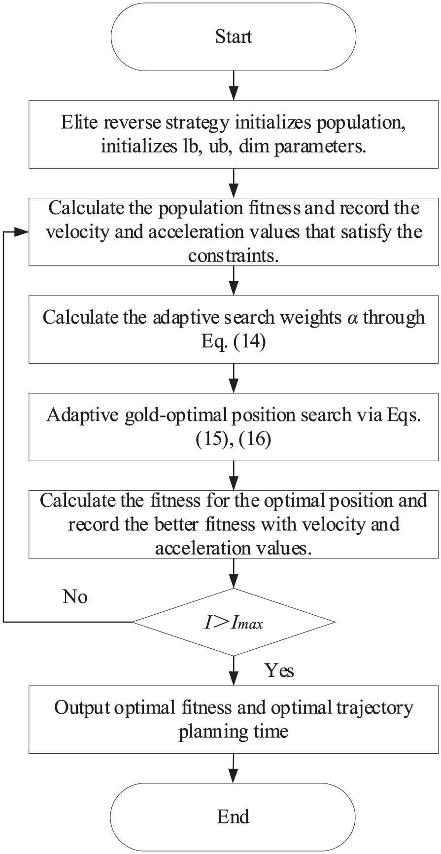
AGS algorithm trajectory planning flowchart.

Time-optimized model

In industrial production, in order to improve the efficiency, several factors such as energy consumption, time, speed, and resistance need to be considered, among which time is a frequently concerned factor. To study the time optimization problem in robotic arm trajectory planning, firstly, based on the establishment of polynomial interpolation model with the consideration of constraints, the core time optimization mathematical model is proposed as shown in equation (6):

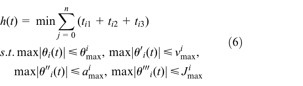
\begin{matrix} h (t) = min \sum_{j = 0}^{n} (t_{i 1} + t_{i 2} + t_{i 3}) \\ s . t . max | θ_{i} (t) | \leq θ_{max}^{i}, max | {θ'}_{i} (t) | \leq v_{max}^{i}, \\ max | {θ ″}_{i} (t) | \leq a_{max}^{i}, max | {θ ″'}_{i} (t) | \leq J_{max}^{i} \end{matrix}

(6)

Where t_i₁, t_i₂, t_i₃ are the planning time of the i (i = 1, 2, …, 6) joints of the robotic arm with three-segment multiform interpolation, where $θ_{max}^{i}, v_{max}^{i}, a_{max}^{i}, J_{max}^{i}$ are the maximum value of the angular displacement constraint, the maximum value of the velocity constraint, the maximum value of the acceleration constraint and the maximum value of the jerk constraint, respectively, and the time optimization is to optimize the sum of all the time to the minimum value, in order to ensure the solving accuracy and the efficiency of the solution, the constraints need to be the maximum value of the absolute value of position, velocity, and acceleration. In order to ensure the accuracy and efficiency of the solution, the constraints need to derive the maximum value of the absolute value of the position, velocity, acceleration, and jerk, this constraint can effectively avoid the mechanical arm in the actual trajectory planning process due to the impact, resistance, and vibration caused by the damage and aging of the equipment, so as to ensure the stability and safety of the mechanical arm in the work process.

Adaptive Gold Search algorithm with trajectory optimization

Elite reverse population initialization

Meta-heuristic optimization algorithms first need population initialization to confirm the initial position of each population. Opposition-based Learning (OBL)²⁸ is an effective method to improve the searching ability of stochastic search algorithms, the core of which is: Assuming $s_{i} = (s_{i, 1}, s_{i, 2}, \cdot \cdot \cdot s_{i, A}) (i = 1, 2 \cdot \cdot \cdot, N)$ is an individual in the A-dimensional search space, which has an upper boundary of lb_j, and a lower boundary of ub_j, and the j-dimensional vector $s_{i, j}$ (j = 1, 2 …, A) of the solution $S_{i}$ is selected as the initialization object, the mathematical model of the inverse solution $s'_{i} = (s'_{i, 1}, s'_{i, 2}, \cdot \cdot \cdot, s'_{i, A})$ is shown in equation (7):

s'_{i, j} = δ (l b_{j} + u b_{j}) - s_{i, j}

(7)

where δ is a moderating factor and is a random value on the interval [0, 1]. Although this method enlarges the search space, it is not applicable to local exploitation and global equilibrium. Therefore, on this basis, this paper introduces the Elite Inverse Strategy (EIS) to improve it, and when the required inverse solution $s'_{i, j}$ exceeds the range of the predefined search space, it will be transgressed, and the solution will be adjusted to the legal search interval:

s'_{i, j} = r (l b_{j}, u b_{j}), (s'_{i, j} < l b_{j} or s'_{i, j} > u b_{j})

(8)

where $r (l b_{j}, u b_{j})$ is a random value on the interval $[l b_{j}, u b_{j}]$ . And to improve the quality of the solution, the population was screened for elite individuals and then reorganized into elite populations. The basic steps to initialize the population by elite reverse strategy are as follows:

(1) After completing the initialization operation of the population S, screen the N/2 individuals with optimal fitness from the population S based on the fitness evaluation criterion.

(2) Solve the inverse population $P'$ of the elite population P according to equations (7) and (8).

(3) Combine population S with the reverse population $P'$ to form a new population, and then select the N individuals with optimal fitness from it to form the population $S_{p'}$ again.

This strategy can improve the ability of the algorithm to search globally and realize global convergence.

Adaptive inertia weights

Early after population initiation, individual patterns concentrate around high-fitness individuals, causing fast velocity decreases. If the inertia weight is persistently low, the population has limited exploitation capacity, causing early convergence and failure to escape local optima. To assure convergence speed, a nonlinear adaptive inertia weight is used to help individuals quickly reach ideal regions.

In order to describe the change of the overall fitness value during the evolution of the population, the definition of evolutionary dispersion is given. The ratio of the standard deviation of the fitness value of the population in generation n to that of the population in generation (n−1) is defined as the evolutionary dispersion k(n):

{\begin{matrix} k (n) = 1, n = 1 \\ k (n) = \frac{S (n)}{S (n - 1)}, n > 1 \end{matrix}

(9)

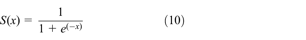
In meta-heuristic algorithms, commonly used inertia weights include Exponential Decreasing Inertia Weight (EDIW),²⁹ Cosine Decreasing Inertia Weight (CDIW),³⁰ etc., which use exponential function and cosine function to construct the inertia weights respectively, but there is a lack of a balanced transition mechanism between the early stage of the algorithm and the late stage of the algorithm, and it is easy to lack of dynamic feedback on the actual state of the algorithm. Sigmoid function is commonly used in neural networks to construct neuron activation function,³¹ which can realize adaptive switching between global exploration and local development, so this paper introduces the Sigmoid function to construct a balanced transition mechanism, which is defined as:

S (x) = \frac{1}{1 + e^{(- x)}}

(10)

Jointly evolve the dispersion k(n) and S function, set the maximum and minimum inertia weights $ω_{max}, ω_{min}$ . In order to ensure that the function adjusts the parameters adaptively, an adjustment coefficient commonly used in the algorithm is introduced: the damping factor b,³² and combined with the evolutionary algebra T yields the nonlinear Dynamic Adaptive Inertia Weight factor (DAIW) computed as:

ω (n) = ω_{max} + (ω_{min} - ω_{max}) \frac{1}{1 + e^{[- 10 b (\frac{2 p}{k (n) \cdot T} - 1)]}}

(11)

where n is the number of iterations. The traditional algorithm³³ needs to set the variable α for improving the result of the new position X_i in the search space before finding the optimal position through iteration, set the iteration to end after I_max times, and introduce a loop counter p to record the number of iterations, whose expression is:

α = (2 - (\frac{p}{\frac{I_{max}}{2}}))

(12)

where the variable α takes values ranging from 0 to 2. This value decreases sharply with each iteration in the loop. This α-scheduling described above for the complex high-dimensional optimization problem of optimal robot arm trajectory planning time, in addition to the ease of falling into the local optimum, the accuracy of the later search is also difficult to be solved by the traditional meta-heuristic. Therefore, the adaptive search weight α is changed to that shown in equation (13):

α = 2 - 2 (\frac{2}{1 + e^{(- 10 \cdot r (\frac{2 p}{I_{max}} - 1))}})

(13)

where r is the damping factor taken between [0, 1]. This strategy ensures that the group position is adjusted while speeding up the convergence rate and ensuring the efficiency of the computation.

Gold global optimal position search

The convergence accuracy and speed of the swarm intelligence algorithm may be significantly impacted by an overly aggressive search strategy or an improper parameter setting, which fails to fully investigate the entire search space despite the introduction of adaptive inertia weights. The traditional algorithm uses a random search for the optimal individual position in the search space, introduces a random search parameter λ based on the product of the minimum search time T_min and the variable α, and then derives the optimal position search expression from the optimal position P_b found in the search area during the development phase as shown in equation (14):

{X_{i}}^{n} = λ \cdot (T_{min} \cdot α) + P_{b}, (i = 1, 2 \cdot \cdot \cdot m)

(14)

where λ is a random value between [1, m] and m is the variable dimension. The Golden Search Optimization Algorithm (GSO)³⁴ can effectively explore the whole search space by adjusting the search behavior through adaptive step size and transfer operator, but this mechanism combines two functions, sine and cosine, to calculate the step size, which leads to high computational complexity and affects the algorithm’s optimization efficiency.

To address this problem, the algorithm in this paper adopts the golden sinusoidal variation strategy to improve the convergence accuracy of the algorithm. First only the better synergistic sinusoidal function is used for the position search, and at the same time, the introduction of the golden section coefficients x₁, x₂, to narrow down the search range and guide the individual to approach the optimal solution, so as to improve the search mechanism of the optimal position, and set the representation coefficients of the distance and direction, R₁ and R₂, respectively, to take the value between $[0, 2 π]$ and $[0, π]$ , to ensure that the correctness of the moving distance and direction. The mathematical model of location search strategy is shown in equation (15):

x_{i}^{n + 1} = x_{i}^{n} \cdot | \sin (R_{1}) | + R_{2} \cdot \sin (R_{1}) \cdot | x_{1} \cdot P_{i}^{n} - x_{2} \cdot x_{i}^{n} |

(15)

where $P_{i}^{n}$ denotes the optimal position of the ith population individual at the nth iteration. x₁, x₂ expressions are shown in equation (16):

{\begin{matrix} x_{1} = - π + (1 - τ) \cdot 2 π \\ x_{2} = - π + τ \cdot 2 π \end{matrix}

(16)

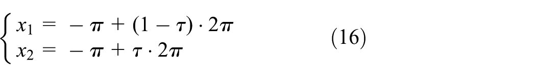
where τ is the golden section number, and the irrational number of $(\sqrt{5} - 1) / 2$ is used here, the combination of golden section coefficients and sinusoidal oscillations significantly improves local exploitation and convergence accuracy. By applying the above strategy, it is possible to avoid the algorithm from falling into the local optimum, improve the convergence accuracy and speed of the algorithm, improve the stability of the robotic arm when it is working, and realize the time-seeking optimization.

AGS algorithm trajectory planning process

According to the above theoretical basis, the steps of AGS algorithm applied to robotic arm time-optimal trajectory planning are as follows:

Step 1: The elite inverse strategy initializes the population overall, initializes the positions of the population as well as the individuals, and initializes the values of the variables lb, ub, dim, and sets the maximum iteration value;

Step 2: Enter the loop, calculate the fitness value h(t) of the population according to equation (6), compare the velocity and acceleration that satisfy the condition, and then update the optimal fitness of the population and record it;

Step 3: Calculate the adaptive search weights according to equation (13);

Step 4: Perform adaptive gold optimal position search according to equations (14) and (15);

Step 5: Calculating the fitness for the optimal position, comparing the fitness that meets the constraints with the optimal fitness recorded in step 2, and recording the better fitness value with the velocity and acceleration values;

Step 6: According to the maximum iteration value set in step 1, determine whether the current maximum iteration value has been reached, and if it has been reached, exit the iteration, and output the optimal population fitness value and the optimal time value of the robotic arm in the trajectory planning process, and plan the optimal trajectory of the robotic arm according to the optimal time.

The algorithm trajectory planning process is shown below:

Algorithm validation and experimental analysis

Algorithm validation results

To validate the reliability and correctness of the AGS algorithm, the simulation experiments in this paper are based on Windows 10 with 64-bit operating system, 3. 2 GHz main frequency and 16GB RAM, and programmed with MATLAB R2020a software. This study conducts a comparative analysis of PSO algorithm, GWO algorithm, GA algorithm, GOOSE algorithm, and AGS algorithm using four benchmark functions from CEC2005, Set the PSO algorithm as follows: the number of population clusters is 30, the weight coefficient ω = 0.7, the learning factor c₁ = 4, c₂ = 3; set the parameters of GA algorithm as follows: the crossover probability p_c = 0.7, and the mutation probability p_m = 0.05; set the parameters of GWO algorithm as follows: the convergence factor a = 2; set the initial parameters of the Goose algorithm as follows: p = r = c = 0.5, and the variable dimensions are 3; and the parameters of golden sinusoidal mutation strategy is parameterized by x₁ = −0.741 and x₂ = 0.741. Each separate run uses a distinct random seed to reflect algorithm randomness. Based on 30 independent runs’ final fitness values, the optimum, worst, mean, and standard deviation are determined, and convergence curves are presented to show convergence performance. Finally, the optimal, worst, mean, and standard deviation values are compared to evaluate performance. Table 1 lists selected test functions and Table 2 summarizes comparison results:

Table 1.

Standard test function.

Types	Function number	Test function	Dimensions	Search area
Unimodal function	F1	$F_{1} (x) = \sum_{i = 1}^{n} x_{i}^{2}$	30	[−100, 100]
Unimodal function	F2	$F_{2} (x) = \sum_{i = 1}^{n} \| x_{i} \| + Π_{i = 1}^{n} \| x_{i} \|$	30	[−10, 10]
Multimodal function	F6	$F_{6} (x) = \sum_{i = 1}^{n} {([x_{i} + 0.5])}^{2}$	30	[−100, 100]
Multimodal function	F7	$F_{7} (x) = \sum_{i = 1}^{n} {ix}_{i}^{4} + random [0, 1)$	30	[−1.28, 1.28]

Table 2.

Algorithm test result.

Function	Result	PSO	GA	GWO	GOOSE	AGS
F1	Optimal	2.6132 × 10⁻¹	1.8765 × 10³	2.7006 × 10⁻²⁸	−2.2522 × 10⁻¹	−7.9359 × 10⁻⁸²
	Worst	3.0157 × 10⁻¹	4.9256 × 10³	7.8711 × 10⁻²⁸	1.1614 × 10⁻²	−2.8429 × 10⁻⁸⁴
	Mean	2.8145 × 10⁻¹	3.4010 × 10³	5.2858 × 10⁻²⁸	−1.0680 × 10⁻¹	−3.9822 × 10⁻⁸²
	Standard deviation	2.8462 × 10⁻²	2.1560 × 10³	3.6560 × 10⁻²⁸	1.6747 × 10⁻¹	5.5915 × 10⁻⁸²
F2	Optimal	1.2477 × 10⁻¹	1.8333 × 10¹	3.5738 × 10⁻¹⁷	4.5491 × 10⁰	−8.0469 × 10⁻⁸⁰
	Worst	2.1536 × 10⁻¹	2.5729 × 10¹	6.9682 × 10⁻¹⁷	7.0843 × 10⁰	1.0260 × 10⁻⁸⁴
	Mean	1.7006 × 10⁻¹	2.2031 × 10¹	5.2710 × 10⁻¹⁷	5.8167 × 10⁰	−4.0234 × 10⁻⁸⁰
	Standard deviation	6.4056 × 10⁻²	5.2301 × 10⁰	2.4002 × 10⁻¹⁷	1.7927 × 10⁰	5.6901 × 10⁻⁸⁰
F6	Optimal	1.6856 × 10⁻¹	6.9564 × 10³	5.0530 × 10⁻¹	−5.5667 × 10⁻¹	−2.9875 × 10⁻¹
	Worst	3.2515 × 10⁻¹	7.3950 × 10³	1.2541 × 10⁰	−4.6582 × 10⁻¹	−2.9848 × 10⁻¹
	Mean	2.4686 × 10⁻¹	6.9564 × 10³	8.7972 × 10⁻¹	−4.8625 × 10⁻¹	−2.9861 × 10⁻¹
	Standard deviation	1.1072 × 10⁻¹	6.2014 × 10²	5.2951 × 10⁻¹	2.8889 × 10⁻²	1.8685 × 10⁻⁴
F7	Optimal	3.8380 × 10⁻²	3.5147 × 10⁻¹	2.7801 × 10⁻³	3.6238 × 10⁻¹	−5.0031 × 10⁻⁴
	Worst	6.1371 × 10⁻²	1.1997 × 10⁰	4.5159 × 10⁻³	4.3126 × 10⁻¹	3.8640 × 10⁻⁴
	Mean	4.9875 × 10⁻²	7.7561 × 10⁻¹	3.6480 × 10⁻³	3.9682 × 10⁻¹	−2.3083 × 10⁻⁴
	Standard deviation	1.6257 × 10⁻²	5.9982 × 10⁻¹	1.2274 × 10⁻³	4.8709 × 10⁻²	3.8109 × 10⁻⁴

The single-peak function mainly tests the convergence speed and accuracy of the algorithm, while the multi-peak function mainly tests the global optimization ability of the function. By analyzing Table 2, it can be seen that in the F1 function, the optimal value and the worst value of AGS are extremely close to the theoretical optimal value of 0, and the average value and the standard deviation are in a very low order of magnitude; in contrast, the precision of the results of PSO, GA, GWO, GOOSE is lower than that of other algorithms by dozens of orders of magnitude; also in the F2 function, the optimal value, the worst value, the average value, and the standard deviation of AGS are also tens of orders of magnitude smaller than those of other algorithms, which proves the advantages of AGS in terms of convergence accuracy and convergence speed. In the multi-peak function F6, the optimal value, the worst value, and the average value of AGS are very close to each other, and all of them are negative, and the standard deviation is also in a very low order of magnitude, indicating that the algorithms can always find very similar, high-quality solutions, and GOOSE also finds a negative solution, but the difference between its optimal value and the worst value is relatively large, and the stability is not as good as that of AGS, and the results of PSO, GA, and GWO are all positive, and the precision and stability are tens of orders of magnitude worse than AGS; also in function F7, the optimal value, mean, and standard deviation of AGS are significantly better than those of other algorithms, and although the worst value is positive, its absolute value is extremely small and is in the same order of magnitude as the optimal value. In the multi-peak function AGS is the only algorithm whose average performance is better than 0, and the very small absolute value and very low standard deviation indicate that AGS can find a solution very close to or even better than 0 in most cases, which proves that AGS has a good global optimization ability in the complex search space. The benchmark function image and the convergence curve of the algorithm are shown in Figure 3:

Figure 3.

Reference function convergence curve: (a) F1 convergence curve, (b) F2 convergence curve, (c) F6 convergence curve, and (d) F7 convergence curve.

By analyzing Figure 3, it can be seen that at the beginning of iteration, the AGS algorithm has a faster descent speed, and has a better optimization accuracy compared with the remaining four algorithms. And the application of population initialization elite inverse strategy and nonlinear descent strategy makes the AGS algorithm converge faster, and it is not easy to fall into the local optimum, as can be seen from the curves of PSO, GA, GOOSE, and GWO in the figure, the four algorithms are easy to fall into the local optimum. In the late iteration, the results of the AGS algorithm tend to stabilize, and finally converge to an optimal value, which indicates that the introduction of the gold sinusoidal variation strategy improves the algorithm’s optimization ability, so that the results do not fluctuate. In summary, the AGS algorithm has better optimization ability and convergence accuracy.

Experimental design

The experimental system in this paper mainly consists of three parts: Upper computer, Communication module, and Driver module. The Upper computer is responsible for the key tasks of control program writing and signal processing, and its output value is transmitted to the CAN bus through the CAN intelligent adapter. The Upper computer adopts Windows system, the control program writing and communication interface are realized by Python, and the CAN intelligent adapter selects the USBCAN driver card, the rate reaches 1 Mbps. The Driver module selects the Cyber-Gear micromotor, and builds the CyberGear six-axis tandem robotic arm body through modeling, and its specific parameters are shown in Table 3:

Table 3.

Basic parameters of robotic arm.

Parameters	Numerical value
Motor weight	317 ± 3 g
Baud rate	1 Mbps
Rated voltage	24 VDC
Rated load	4 N m
Torque maximum speed	240 rpm ± 10%
Maximum speed	296 rpm ± 10%
Communication method	CAN
Encoder type	Single-coded absolute value
Encoder resolution	14bit

The experimental platform constructed is shown in the Figure 4:

Figure 4.

Robotic arm experiment platform.

In this paper, we use the standard DH method to analyze the kinematics of the robotic arm, and solve the length a_i of the connecting rod, the torsion angle α_i of the connecting rod, the offset distance d_i of the connecting rod, and the joint angle θ_i. Meanwhile, in order to ensure the stability and safety of the robotic arm in the process of the actual trajectory planning, as well as to ensure the accuracy of the experiment, the maximum speed limitations of the various joints of the robotic arm are: 148, 109, 214, 368, 385, 462°/s. The resulting kinematic parameters of the robotic arm are shown in Table 4:

Table 4.

DH parameter table.

Joint i	a_i (mm)	α_i (°)	d_i (mm)	θ_i (°)	Joint range (°)
1	0	0	46	θ ₁	±360
2	0	90	85	θ ₂	0–255.22
3	145	180	0	θ ₃	0–108.3
4	145	180	0	θ ₄	0–230.63
5	145	180	0	θ ₅	0–144.42
6	145	180	0	θ ₆	±360

From the 3-5-3 hybrid interpolating polynomial schematic diagram, we can see that we need to select four path points in the joint space as the four interpolation points for trajectory planning, and the angle of the corresponding joint position of each interpolation point is shown in Table 5, as well as the corresponding actual location is shown in Figure 5:

Table 5.

Joint position.

Interpolation point	Joint position /(rad)
	Joint 1	Joint 2	Joint 3	Joint 4	Joint 5	Joint 6
1	0	0	0	0	0	0
2	0.7854	0.5236	0.7854	0.3927	0.5236	0.3927
3	1.0472	0.5236	0.6283	0.7854	0.7854	0
4	0	0	1.0472	1.5708	0	0

Figure 5.

Physical location: (a) position 1, (b) position 2, (c) position 3, and (d) position 4.

Figure 5(a) figure for the zero position of the robot arm, is the entire trajectory planning process of the mechanical zero point, (b), (c) figure for the movement process of the two interpolation points, as shown in the figure of the two positions of the robot arm are smooth to reach the predetermined position, and the joints have not exceeded the range of joint movement, (d) figure for the movement of the termination point, at this time, the speed of all the joints and acceleration are 0. The entire movement process of the robot arm is smooth and jitter free, and the stability of the robot is good.

Test results and analysis

In order to effectively verify the reliability and effectiveness of the AGS algorithm in robotic arm trajectory planning, the optimized optimal time value of the AGS algorithm is compared and verified with the optimized optimal time value of the AGS algorithm, GA algorithm, GWO algorithm, and GOOSE algorithm. The periods of time before optimization are t₁ = t₂ = t₃ = 2 s, meanwhile, in order to ensure the correctness of the experimental results and to avoid chance, the experiment will be repeated for five times, and the average value of the five experimental values will be taken for comparison, and the experimental results are shown in Table 6:

Table 6.

Time optimization results (unit: s).

Frequency	PSO	GA	GWO	GOOSE	AGS
1	7.1479	6.8732	6.3526	6.4494	6.0202
2	6.8507	6.9987	6.5343	6.2770	5.9641
3	7.3188	7.0453	6.4823	6.3873	6.0188
4	6.7898	6.8352	6.3445	6.2757	5.7525
5	6.5619	7.0363	6.0345	6.1563	6.2963
Mean	6.9338	6.9577	6.3496	6.3091	6.0103

As can be seen from the data in Table 6, the optimization effect of the AGS algorithm shortens the optimization time value of the remaining four algorithms by an average of 13.31%, 13.61%, 5.34%, and 4.73%, respectively, and the time optimization effect is significant. In order to further verify the advantages of AGS algorithm with high convergence accuracy and not easy to fall into local optimum, the adaptation curves of the six joints in the trajectory planning process are compared with the AGS algorithm, GOOSE algorithm, GA algorithm, GWO algorithm, and PSO algorithm, respectively, and the comparison is shown in Figure 6:

Figure 6.

Joint fitness curve.

The change contours of joint fitness are compared in Figure 6 when five algorithms, namely AGS, GOOSE, GA, GWO, and PSO, are optimized for robotic arm trajectory planning. The analysis shows that: the AGS curve exhibits the steepest descending slope at the beginning of the iteration and takes the lead to reach a steady state between 10 and 20 generations into a low adaptation level, in contrast, the GOOSE, GA, GWO, and PSO curves reach a steady state with a delay of about 5, 30, 10, and 30 generations, respectively, which verifies that the AGS has a faster convergence speed, and the AGS is finally stabilized at the lowest adaptation value between 0.8 and 2.0, which is significantly lower than the adaptation level of other algorithms after stabilization, the PSO and GA curves stagnate in the middle of the iteration, around the higher adaptation level of 1.4–2.6, and the GOOSE and GWO curves also fluctuate slightly around the level close to 0.8, which shows the characteristic of falling into the local optimum, whereas the AGS overcomes the problem of being prone to falling into the local optimum. According to quantitative calculations, the convergence accuracy of AGS is enhanced by 55.1%, 16.03%, 16.53%, and 53.06% on average when compared to PSO, GOOSE, GA, and GWO. This supports the assertion that AGS has a stronger global optimization ability, a faster convergence speed, and a higher convergence accuracy.

Meanwhile, under the constraints of joint velocity, joint acceleration, and joint jerk of the robotic arm, the convergence of angular displacement, velocity, acceleration, and jerk curves of the robotic arm after optimization as well as the time needed for convergence are used to verify the convergence effect of the AGS algorithm, and the curves of angular displacement, angular velocity, angular acceleration, and angular jerk are shown in Figures 7 to 10 after optimization:

Figure 7.

Joint position curve of each joint.

Figure 8.

Joint velocity curve of each joint.

Figure 9.

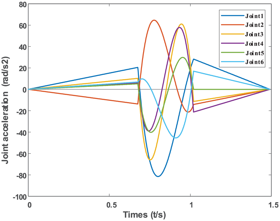
Joint acceleration curve of each joint.

Figure 10.

Joint jerk curve of each joint.

As can be seen from Figures 7 to 10, the displacement curves of all six joints are smooth and continuous single-valued functions without any breakpoints or non-conductive cusps, and the curve morphology conforms to the typical smooth trajectory characteristics, which ensures the coherence of the joint motions. Secondly, the velocity curves of each joint are continuous and change gently, and all the velocity curves do not have instantaneous jumps, which avoids the theoretical infinite acceleration. The acceleration curves also maintain continuity, and the curve changes relatively gently without violent pulse-type spikes, indicating that the motion process has little impact. Although the acceleration curve has abrupt changes at the time nodes, the overall trajectory planning process is relatively smooth and there is no joint jitter. Finally, the displacement, velocity, acceleration, and jerk constraints of the robotic arm satisfy the constraints of the temporal optimization model, implying that the motion of the robotic arm is within the safety range, thus verifying the feasibility and accuracy of the proposed algorithm optimization scheme.

Obstacle avoidance performance test

In order to further verify the applicability and accuracy of the AGS algorithm in the offline programming system of the robotic arm, the real environment of the robotic arm is constructed in the V-REP software through the URDF file, and an ordinary cylinder is used as an obstacle, and obstacle avoidance trajectory planning is carried out by using the AGS algorithm, so as to validate the obstacle avoidance performance of the AGS algorithm applied in the offline programming system.

Set the coordinates of the obstacle as well as the coordinates of the robot arm’s obstacle avoidance path point as shown in the Table 7 below:

Table 7.

Keypoint coordinate values.

Coordinate node	X-coordinate point	Y-coordinate point	Z-coordinate point
1	0.164	0.011	0.042
2	0.196	0.011	0.319
3	0.230	−0.178	0.233
Obstacle	0.160	−0.050	0.125

By planning the same obstacle avoidance path without AGS (only 3-5-3 trajectory planning) and with AGS, the water bottle is used as a cylindrical obstacle, the parameter settings and environment configuration are the same as in the previous section, and the number of experiments is set to 30, and the data comparison between the two cases is shown in Table 8, and the optimal obstacle avoidance obtained by AGS is shown in Figures 11 and 12:

Table 8.

Comparison of two types of scene data.

Scenes	Minimum collision distance (m)	Terminal error (mm)	The number of collisions with obstacles
Without AGS	0.197	6.745	12
With AGS	0.458	2.013	3

Figure 11.

Simulation experiment obstacle avoidance effect: (a) path point 1, (b) path point 2, and (c) path point 3

Figure 12.

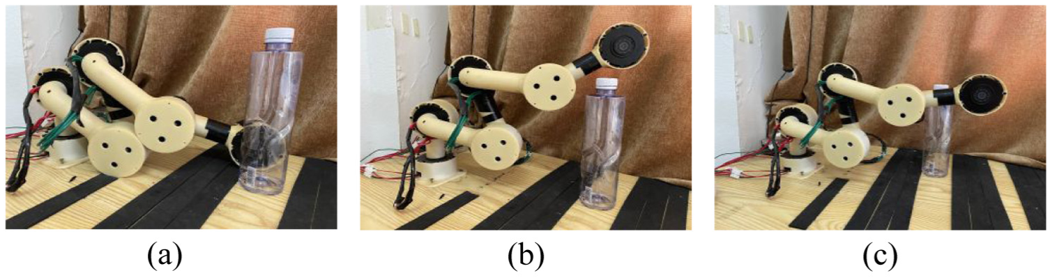
Physical experiments obstacle avoidance effects: (a) path point 1, (b) path point 2, and (c) path point 3.

Analyzing Table 8 shows that the minimum collision distance with AGS is significantly more stable and farther away and safer than without AGS, and the end error with AGS is smaller than without AGS, which indicates that the former has a higher trajectory accuracy and a more stable performance, and the number of collisions with obstacles with AGS is much smaller than without AGS, which indicates that the algorithmic searching ability of AGS is stronger and can ensure the efficient as well as safe operation tasks.

As can be seen from Figures 11 and 12, the robotic arm is at zero position at path point 1, and when the robotic arm moves from zero position to path point 2 near the obstacle, the obstacle is detected, and the trajectory of the robotic arm changes, running smoothly from the left front of the robotic arm to the right front, and finally arriving at the target position, and the whole process has no collision with the obstacle and the trajectory is smooth and continuous. The path effects of Figure 11(a) to (c) diagrams also keep correspondence with Figure 12(a) to (c) diagrams. It is proved that the AGS algorithm can adapt to the complex environment in the offline programming system of the robotic arm and make the robotic arm have better obstacle avoidance performance, which further verifies the high applicability of the AGS algorithm in practical applications.

Conclusions

In order to solve the problem of timeliness of robotic arm trajectory to efficiently complete complex industrial production tasks, an AGS algorithm is proposed to optimize the robotic arm trajectory planning time to solve the optimal time of robotic arm joint trajectory planning to achieve the following effects:

(1) The proposed algorithm accomplishes global optimization, which guarantees high efficiency in robotic arm operations. The AGS algorithm generates an average total planning time of 6.0103 s, whereas PSO, GOOSE, GA, and GWO generate average times of 6.9338, 6.3091, 6.9577, and 6.3496 s, respectively. As a result, the proposed algorithm exhibits average performance enhancements of 13.31%, 13.61%, 5.34%, and 4.73% over PSO, GOOSE, GA, and GWO in the optimization of the total planning time for the three-segment robotic arm.

(2) In this paper, the AGS algorithm optimizes the adaptability curve of each robotic arm joint with a faster convergence speed and higher convergence accuracy than the PSO algorithm, the GOOSE algorithm, the GA algorithm, and the GWO algorithm. The convergence accuracy of the AGS algorithm is improved by 55.1%, 16.03%, 16.53%, and 53.0%, respectively.

(3) The algorithm in this paper has good convergence speed, and the optimized angular displacement, velocity, acceleration, and jerk curves of the AGS algorithm are continuous, smooth, and mutation-free, so the robotic arm does not have velocity mutation during movement, improving safety and stability. In the robotic arm offline programming system, it can improve obstacle avoidance and adapt to complex environments.

The AGS algorithm is capable of effectively resolving the timeliness issue in robotic arm trajectory planning when the motion constraints are satisfied, as evidenced by the experimental results. It effectively mitigates the conventional optimization algorithms’ common deficiencies, including a propensity to converge to local optima, a sluggish convergence speed, and low convergence accuracy, while simultaneously reducing the operation time. The adaptive golden search algorithm was implemented in subsequent research to optimize obstacle avoidance strategies and reduce trajectory energy consumption for robotic arms, with an emphasis on enhancing the algorithm’s search capabilities and enhancing the efficacy of robotic arm joints.

Footnotes

Handling Editor: Hsiu-Ming Wu

ORCID iDs

Chen Lifeng

Mao Jiaxin

Funding

The authors disclosed receipt of the following financial support for the research, authorship, and/or publication of this article: The paper was funded by the Hunan Provincial Natural Science Foundation of China (Grants Nos. 2024JJ8275 and 2024JJ2031).

Declaration of conflicting interests

The authors declared no potential conflicts of interest with respect to the research, authorship, and/or publication of this article.

References

Zhang

Feng

Bano

, et al. Soil water content estimation by using ground penetrating radar data full waveform inversion with grey wolf optimizer algorithm. Vadose Zone J 2024; 24(1): e20379.

Shi

Jin

, et al. Design of intelligent firefighting and smart escape route planning system based on improved ant colony algorithm. Sensors 2024; 24(19): 6438.

Xue

Yan

Jia

, et al. Photovoltaic power prediction based on improved gray wolf algorithm and optimization of long short-term memory network. Acta Sol Energy Sin 2023; 44(7): 207–213. (in Chinese)

Holland

JH.

Genetic algorithms. Sci Am 1992; 267(1): 66–73.

Storn

Price

Differential evolution–a simple and efficient heuristic for global optimization over continuous spaces. J Glob Optim 1997; 11: 341–359.

Glover

Tabu search: a tutorial. Interfaces 1990; 20(4): 74–94.

Zhu

Pan

Improved genetic algorithm for solving robot path planning based on grid maps. Mathematics 2024; 12(24): 4017.

Damage detection in steel structures using wavelet transformation and generalized genetic algorithm. ce/papers 2025; 8(2): 897–904.

Kennedy

Eberhart

Particle swarm optimization. In: ICNN’95-international conference on neural networks, Perth, WA, Australia, 27 November–1 December 1995, pp.1942–1948. New York: IEEE.

10.

Dorigo

Maniezzo

Colorni

Ant system: optimization by a colony of cooperating agents. IEEE Trans Syst Man Cybern B Cybern 1996; 26(1): 29–41.

11.

Mirjalili

Lewis

Grey wolf optimizer. Adv Eng Softw 2014; 69(3): 46–61.

12.

Zhao

Tang

WS.

Monkey algorithm for global numerical optimization. J Uncertain Syst 2008; 2(3): 165–176.

13.

Figueiredo

Ludermir

Bastos-Filho

Many objective particle swarm optimization. Inf Sci 2016; 374(20): 374115–374134.

14.

Jiang

Huang

, et al. An improved particle swarm optimization algorithm. Appl Math Comput 2007; 193(1): 231–239.

15.

Abdel-Basset

Mohamed

Jameel

, et al. Spider wasp optimizer: a novel meta-heuristic optimization algorithm. Artif Intell Rev 2023; 56(10): 11675–11738.

16.

Abdel-Basset

Mohamed

Jameel

, et al. Nutcracker optimizer: a novel nature-inspired metaheuristic algorithm for global optimization and engineering design problems. Knowl Based Syst 2023; 262(2): 110248.

17.

Trojovská

Dehghani

Trojovský

, et al. Zebra optimization algorithm: a new bio-inspired optimization algorithm for solving optimization algorithm. IEEE Access 2022; 10(4): 49445–49473.

18.

Luo

Particle swarm Optimization for Dynamic Adjustment of inertia weights. Appl Comput Syst 2019; 28(12): 184–188. (in Chinese)

19.

Yang

Yao

, et al. Optimal trajectory planning for robotic arm based on improved dynamic multi-population particle swarm optimization algorithm. Int J Adv Comput Sci Appl 2024; 15(5): 710–718.

20.

Wang

Guan

Improved whale optimization algorithm for high-dimensional optimization problems. J Comput Sci Explor 2022; 16(12): 2890–2902. (in Chinese)

21.

Long

Zhao

Improved grey wolf optimization algorithm for constrained optimization problems. J Comput Appl 2015; 35(9): 2590–2595. (in Chinese)

22.

Bai

Liu

Multi-objective artificial bee algorithm based on decomposition by PBI method. Appl Intell 2016; 45(4): 976–991.

23.

Liu

Yang

Liu

, et al. An improved ant colony algorithm for robot path planning. Soft Comput 2017; 21(61): 5829–5839.

24.

Tanyildizi

Demir

Golden sine algorithm: a novel math-inspired algorithm. Adv Electr Comput Eng 2017; 17(2): 71.

25.

Ali

Annuar

Miskon

MF.

Trajectory planning for exoskeleton robot by using cubic and quintic polynomial equation. Int J Appl Eng Res 2016; 11(13): 7943–7946.

26.

Lian

Xiao

, et al. Cubic spline interpolation-based robot path planning using a chaotic adaptive particle swarm optimization algorithm. Math Probl Eng 2020; 1(2020): 1849240.

27.

Hongsheng

Yunhe

Wei

, et al. Trajectory planning for industrial robots for NURBS free curve. Inf Control 2017; 46(2): 129–135.

28.

Tizhoosh

. Opposition-based learning: a new scheme for machine intelligence. In: Proceedings of the international conference on computational intelligence for modeling control and automation, Vienna, Austria, 28–30 November 2005, pp.695–701. New York: IEEE.

29.

Bai

Generalized radial basis function neural network based on an improved dynamic particle swarm optimization and AdaBoost algorithm. Neurocomputing 2015; 152(25): 305–315.

30.

Nishat

Sakib

Rahman

, et al. Applying particle swarm optimization for investigating the stability of DC-DC buck-boost converter: a software based approach. Int J Model Simul 2024; 23(15): 1–20.

31.

Youn

Y-R

Hong

Enhancing convolutional neural network performance through optimized sigmoid activation function modeling. Asia Pac J Converg Res Interchange (APJCRI) 2023; 9(10): 51–59.

32.

Dong

XL.

An improved PRP conjugate gradient algorithm with a damping factor within an automatic restarting strategy. J Comput Appl Math 2025; 468: 116638.

33.

Hamad

Rashid

TA.

GOOSE algorithm: a powerful optimization tool for real-world engineering challenges and beyond. Evol Syst 2024; 15(1): 1–26.

34.

Noroozi

Mohammadi

Efatinasab

, et al. Golden search optimization algorithm. IEEE Access 2022; 10: 37515–37532.