Research on water hammer model and pressure pulsation of digital hydraulic valve control system

Abstract

It is found through experiments that the amplitude, waveform and periodicity of the water hammer pressure pulsation under the continuous on/off of the valve in the digital hydraulic system are affected by the frequency of the valve switching valve, which is greatly deviated from the prediction and evaluation results of the traditional water hammer model. Therefore, to improve the prediction accuracy of the pressure pulsation (water hammer) model in continuous switching digital hydraulic systems, this work starts from the fundamental water hammer mechanism. Based on the on/off characteristics of the high-speed switching valve, a relationship is established between the valve opening variation and the valve switching frequency through a time-dependent function. Furthermore, by accounting for the elasticity of the pipe walls and the compressibility of the fluid, a novel model capable of predicting water hammer pressure pulsations under continuous valve switching is constructed. The accuracy of this new model was experimentally verified, demonstrating a prediction error for the system’s water hammer pressure that does not exceed 5%. This research model provides theoretical support for the reliability design of high-speed switch valve hydraulic systems by accurately predicting the water hammer pressure of the system under continuous on/off, and is also of great significance for further in-depth research on digital hydraulic valve systems.

Introduction

Digital hydraulic technology is an inevitable trend to improve the energy efficiency and reliability of traditional hydraulic technology.^1,2 However, the presence of pulsating fluid may cause resonance of system parameters, further damage the pipeline system, reduce the control accuracy of the system and generate vibration noise.^3,4 The water hammer pressure pulsation generated by the on/off characteristics in the digital hydraulic valve control system is an important component of the formation of pulsating fluid. Therefore, the prediction and analysis of water hammer are very important for the construction and operation of digital hydraulic systems, and also have reference significance for further accurate analysis of the impact of different pulsating fluids on pipeline systems. At present, the reservoir – pipeline – valve system is usually used as the research object of water hammer^4–10 as shown in Figure 1. The research conditions are closing the valve port, steady friction and low-velocity micro-compressible fluid.

Figure 1.

The motion state of the fluid after the valve port is closed. ¹

The current research on water hammer is mainly carried out from two aspects: theoretical analysis and experimental research.^11,12 The experimental research method mainly focuses on the improvement of the test bench. Usually, the measurement accuracy of the water hammer pressure of the test bench is improved by correcting the test method^13,14 and optimizing the test equipment, ¹⁵ so as to realize a more accurate analysis of the water hammer phenomenon. With the improvement of the solution method of water hammer model, in order to realize the analysis and prediction of water hammer more efficiently and economically, water hammer research has gradually paid attention to the water hammer model in theoretical analysis.

The common water hammer model research mainly considers the parameter hammer model research mainly considers the parameter changes between the pipeline and the valve, and improves the water hammer model from the aspects of pipeline shape size, material and friction form, so as to improve the accuracy of water hammer prediction and evaluation.^6–18 However due to the lack of consideration of the type of water hammer generated by the valve port switch and the change of local fluid flow in the valve port, the evaluation accuracy of the water hammer model is limited. Therefore, researchers began to analyze the influence of the valve port on the water hammer.^19–21 Xu et al. ²² noted that the influence of the initial opening of the valve port on the change of fluid flow was neglected in the traditional water hammer theory. By combining the kinetic energy equation, a new mathematical model was derived to further analyze the influence of uneven flow caused by different openings of the valve port on the water hammer pressure. It was found that the water hammer pressure value exceeded the traditional Joukowsky theorem by 21%. In order to further determine the error of water hammer pressure between different initial openings, Zhang et al. ²³ studied the direct water hammer pressure generated when the initial opening of the valve port was 100% and 30%. The maximum difference in pressure changes under different openings can reach 10.48%. Subsequently, Mo et al. ²⁴ combined the opening of the valve port with the closing law of the valve port, completed the exploration of the influence law of the amplitude and shape of the water hammer pressure wave, further improved the accuracy of the water hammer model, and realized the prediction and analysis of the water hammer.

In the digital hydraulic valve control system, the valve port needs to be continuously on/off, and the valve port opening also changes continuously with time, which leads to great changes in the research boundary of the existing water hammer, resulting in a periodic alternating water hammer, and a continuous water hammer pressure wave is formed in the pipeline, as shown in Figure 2. The variation of pulsating fluid pressure in the pipeline at different frequencies shown in Figure 2 indicates that water hammer pressure pulsation in digital valve control systems is affected by valve switching frequency. However, current theory shows that the fluctuation of water hammer pressure is not related to the frequency of valve opening/closing. This is because the current water hammer theory is mainly used to analyze the propagation, attenuation and impact of water hammer pressure waves on pipeline vibration after the formation of a single water hammer, as shown in Figure 3. This makes it difficult for current water hammer theory to accurately predict and analyze the continuous water hammer pressure pulsation formed by continuous opening/closing in digital hydraulic valve control systems.

Figure 2.

Continuous on/off continuous water hammer pressure wave.

Figure 3.

Oscillation attenuation water hammer pressure wave.

In order to realize the study of water hammer under continuous switch, this paper starts from the mechanism of water hammer. By considering the change of boundary conditions under continuous switch, the function of continuous change of opening with time is introduced, and a bridge for mechanism analysis of the relationship between continuous switch and boundary conditions is set up. The water hammer model that can calculate the continuous switch is constructed, and the essential relationship between the switching frequency and the water hammer pressure is clarified theoretically. Secondly, the water hammer pressure pulsation test bench is designed to realize the measurement of water hammer pressure pulsation and complete the experimental verification of the model. Finally, through the joint analysis of experiment and simulation, the influence of different switching frequencies on the pressure pulsation of water hammer is explored.

Model establishment and solution

Physical model

Construct a research model as shown in Figure 1, with the upstream starting section being a reservoir and the downstream end being a high-speed switch valve. This is a reservoir valve pipeline system, and make the following assumptions for the research model.^25,26

• (1) The fluid in the pipe is considered as one-dimensional flow, and the velocity and pressure are uniformly distributed on the cross section;

• (2) The friction loss in the model is considered as steady frictional loss;

• (3) The fluid in the tube is always completely filled;

• (4) The model analysis does not consider the phenomenon of column separation;

• (5) Neglecting the influence of gas inside the liquid during model analysis;

• (6) The pipe wall and liquid show linear elasticity;

• (7) Ignoring the pressure change caused by structural vibration.

The cross section of the initial length is intercepted in the pipeline in Figure 1, and the fluid in it is taken as the research object. Figure 4 is the analysis diagram of the interaction between fluid motion and water hammer pressure wave propagation in the pipeline.

Figure 4.

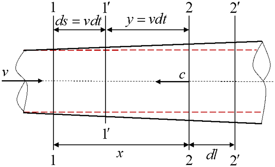
Water hammer wave propagation diagram.

Select a control body of length x, and after time dt, the control bodies of segments 1–2 move to segment 1′–2′, The water hammer pressure wave also propagated to the 1–1′ end face.

During time dt, the forces acting on the control body include pressure at both ends of the cross-section, water pressure on the side, gravity and frictional resistance of the pipe wall. Therefore, the momentum of the control body is^27,28:

$$\begin{array}{c}\mathrm{pA}-(\mathrm{pA}+\frac{\partial \left(\mathrm{pA}\right)}{\partial s}x)+(p+\frac{\partial p}{\partial s}\frac{x}{2})\frac{\partial A}{\partial s}x-\xi \chi x\hfill \\ =\rho (A+\frac{\partial A}{\partial s}\frac{x}{2})x\frac{\mathrm{dv}}{\mathrm{dt}}\hfill \end{array}$$

(1)

where A represents the cross-sectional area of the inner diameter of the pipe; ρ represents density of the fluid; v represents flow velocity; x represents the length of the control body intercepted inside the pipeline; χ represents wetted perimeter; ξ pipe inner wall shear stress. g represents acceleration of gravity, t denotes the unit of time, s represents the unit length along the flow direction.

Within time dt, the control body is considered to flow relative to the pipeline, and the difference in mass of the fluid entering and exiting the control volume should be equal to the increase in fluid mass in the control volume at this time^27,28:

$$\mathrm{Av}\frac{\partial \rho }{\partial s}+\frac{\partial \rho }{\partial t}A+\rho V\frac{\partial A}{\partial s}+\rho \frac{\partial A}{\partial t}+\rho A\frac{\partial v}{\partial s}=0$$

(2)

The basic equation for calculating water hammer can be obtained by using equations (1) and (2), as follows:

$$\begin{array}{c}\frac{\partial p}{\partial x}+\frac{4\xi }{D}+\rho \frac{\mathrm{dV}}{\mathrm{dt}}=0\hfill \\ \frac{1}{\rho }\frac{\mathrm{d}\rho }{\mathrm{d}t}+\frac{1}{A}\frac{\mathrm{d}A}{\mathrm{d}t}+\frac{\partial v}{\partial s}=0\hfill \end{array}$$

(3)

Equation (3), serving as the governing equation for water hammer calculations, is the fundamental model originally developed to solve incompressible water hammer pressure variations. In practical engineering, the changes in fluid density and pipeline elasticity over time and distance are usually considered to ensure the compatibility between the model and reality. The fluid elasticity equation and pipeline elasticity equation are respectively used to represent:

$$\begin{array}{c}\frac{1}{\rho }\frac{\mathrm{d}\rho }{\mathrm{d}p}=\frac{1}{K}\hfill \\ \frac{1}{A}\frac{\mathrm{d}A}{\mathrm{d}p}=\frac{D}{E\delta }\hfill \end{array}$$

(4)

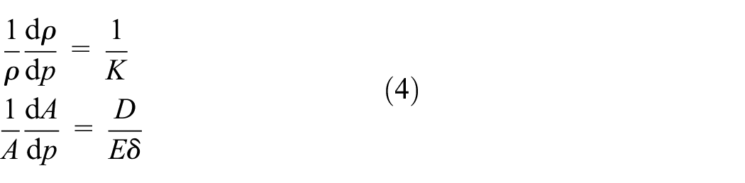
where E represents elastic modulus of pipes; K represents bulk modulus of elasticity of fluid; δ represents pipe wall.

Equation (4) are introduced into equation (3), respectively. The pressure p is represented by the pressure head H, $\xi =\lambda \rho v^2/8$ and $\chi =\pi D=2\sqrt{\pi A}$ are substituted into the motion equation. λ represents drag coefficient. The water hammer equation considering fluid elasticity and pipeline elasticity can be obtained by sorting out:

$$\{\begin{array}{c}\frac{\partial v}{\partial t}+v\frac{\partial v}{\partial s}+g\frac{\partial H}{\partial s}+\frac{\mathrm{Hg}}{\rho }\frac{\partial \rho }{\partial s}+\frac{\lambda v|v|}{4}\sqrt{\frac{\pi }{A}}=0\hfill \\ \frac{\partial H}{\partial t}+v\frac{\partial H}{\partial s}+\frac{\frac{1}{\rho g}-\frac{H}{K}}{\frac{2}{E\delta }\sqrt{\frac{A}{\pi }}+\frac{1}{K}}\frac{\partial v}{\partial s}=0\hfill \\ \frac{\partial \rho }{\partial t}+v\frac{\partial \rho }{\partial s}-\frac{\rho }{(\frac{K}{\rho g}-H)}(\frac{\partial H}{\partial t}+v\frac{\partial H}{\partial s})=0\hfill \\ \frac{\partial A}{\partial t}+v\frac{\partial A}{\partial s}-\frac{\frac{2\mathrm{AK}}{E\delta }\sqrt{\frac{A}{\pi }}}{(\frac{K}{\rho g}-H)}(\frac{\partial H}{\partial t}+v\frac{\partial H}{\partial s})=0\hfill \end{array}$$

(5)

Equation (5) comprises four equations governing four variables: the water hammer piezometric head H, the cross-sectional flow area A, the fluid velocity v and the fluid density ρ. These four unknowns correspond to the four equations, forming a closed system of equations. Consequently, the reformulated system becomes solvable for numerical computation.

Model solving

In the process of solving water hammer problems, the characteristic line method and finite difference method are two commonly used methods. ²⁹ Because the water hammer problem studied in this article takes into account the elasticity of pipelines and fluids, a closed system of 4-equation water hammer equations is formed, and the characteristic line method is not suitable. Therefore, the direct finite difference method is chosen for calculation and solution. Huang ³⁰ found that the diamond format in the direct difference method is not ideal for the calculation of water hammer, so the diffusion format in the linear difference method is adopted. In addition to the Courant condition, the stability conditions of the difference method need to meet: $\mathrm{\Delta }s/\mathrm{\Delta }t\ge {|v\pm \{1/\sqrt{p[(1/K)+(D/E\sigma )]}\}|}_{max}$ .

W represents water level H, cross-sectional area A, flow velocity v or density ρ. $W_i^j$ represents the function value of the cross section i when j, then the partial derivative of W to time is expressed as:

$$\frac{\partial W}{\partial t}\approx \frac{W_i^j-[\alpha W_i^{j-1}+\frac{1-\alpha }{2}(W_{i+1}^{j-1}+W_{i-1}^{j-1})]}{\mathrm{\Delta }t}$$

(6)

Where $\alpha W_i^{j-1}+\frac{1-\alpha }{2}(W_{i+1}^{j-1}+W_{i-1}^{j-1})$ is expressed as the weighted average of three adjacent points on the layer at time j−1, α represents the weighted average of the three adjacent points at the same time, that is, the weighted coefficient. The selection criterion for parameter a is to ensure both compliance with the Courant-Friedrichs-Lewy stability condition and satisfactory computational accuracy. Therefore, a is typically first determined through model-based preliminary calculations, followed by algorithmic optimization to derive the optimal parameter value. ²⁹ The value of α indeed varies depending on changes in the system’s structural parameters, classifying it as a semi-empirical coefficient. In this study, after constructing the model, an iterative loop targeting α was implemented. Through continuous iteration, an optimal value for α was determined. This ensures that the obtained parameter can be effectively applied to the solution of the system’s water hammer pressure by the model under identical structural parameters. The superscript j represents the jth moment, and the subscript i represents the ith node of the pipeline. And equation (6) is only used for solving internal nodes.

The partial differential quotient of W to distance is expressed as the central deviation quotient in the following form:

$$\frac{\partial W}{\partial s}\approx \frac{W_{i+1}^{j-1}-W_{i-1}^{j-1}}{2\mathrm{\Delta }s}$$

(7)

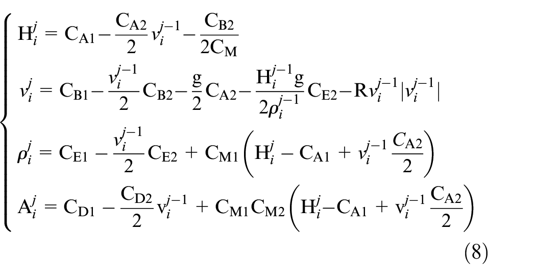
In the process of solving the water hammer model established in this article, it is necessary to discretize the equation system of the model, that is, convert the differential equations into algebraic equations. Then, the diffusion difference scheme is used to solve the model, where the 1−t plane mesh is divided as shown in Figure 5. The final differential format obtained is as follows:

$$\{\begin{array}{c}{\mathrm{H}}_i^j={\mathrm{C}}_{\mathrm{A}1}-\frac{{\mathrm{C}}_{\mathrm{A}2}}{2}{v}_i^{j-1}-\frac{{\mathrm{C}}_{\mathrm{B}2}}{2{\mathrm{C}}_{\mathrm{M}}}\hfill \\ v_i^j={\mathrm{C}}_{\mathrm{B}1}-\frac{v_i^{j-1}}{2}{\mathrm{C}}_{\mathrm{B}2}-\frac{\mathrm{g}}{2}{\mathrm{C}}_{\mathrm{A}2}-\frac{{\mathrm{H}}_i^{j-1}\mathrm{g}}{2{\rho }_i^{j-1}}{\mathrm{C}}_{\mathrm{E}2}-\mathrm{R}{v}_i^{j-1}|v_i^{j-1}|\hfill \\ {\rho }_i^j={\mathrm{C}}_{\mathrm{E}1}-\frac{v_i^{j-1}}{2}{\mathrm{C}}_{\mathrm{E}2}+{\mathrm{C}}_{\mathrm{M}1}({\mathrm{H}}_i^j-{\mathrm{C}}_{\mathrm{A}1}+v_i^{j-1}\frac{C_{\mathrm{A}2}}{2})\hfill \\ {\mathrm{A}}_i^j={\mathrm{C}}_{\mathrm{D}1}-\frac{{\mathrm{C}}_{\mathrm{D}2}}{2}{\mathrm{v}}_i^{j-1}+{\mathrm{C}}_{\mathrm{M}1}{\mathrm{C}}_{\mathrm{M}2}({\mathrm{H}}_i^j-{\mathrm{C}}_{\mathrm{A}1}+{\mathrm{v}}_i^{j-1}\frac{{\mathrm{C}}_{\mathrm{A}2}}{2})\hfill \end{array}$$

(8)

$$\{\begin{array}{c}{\mathrm{C}}_{\mathrm{A}1}=\alpha {\mathrm{H}}_i^{j-1}+\frac{1-\alpha }{2}({\mathrm{H}}_{i+1}^{j-1}+{\mathrm{H}}_{i-1}^{j-1})\hfill \\ \multicolumn{1}{c}{{\mathrm{C}}_{\mathrm{A}2}=\left({\mathrm{H}}_{i+1}^{j-1}{-\mathrm{H}}_{i-1}^{j-1}\right)\frac{\mathrm{\Delta }\mathrm{t}}{\mathrm{\Delta }\mathrm{s}}}\\ \multicolumn{1}{c}{{\mathrm{C}}_{\mathrm{B}1}=\alpha v_i^{j-1}+\frac{1-\alpha }{2}(v_{i+1}^{j-1}+v_{i-1}^{j-1})}\\ \multicolumn{1}{c}{{\mathrm{C}}_{\mathrm{B}2}=(v_{i+1}^{j-1}-v_{i-1}^{j-1})\frac{\mathrm{\Delta }t}{\mathrm{\Delta }s}}\\ \multicolumn{1}{c}{{\mathrm{C}}_{\mathrm{D}1}=\alpha {\mathrm{A}}_i^{j-1}+\frac{1-\alpha }{2}({\mathrm{A}}_{i+1}^{j-1}+{\mathrm{A}}_{i-1}^{j-1})}\\ \multicolumn{1}{c}{{\mathrm{C}}_{\mathrm{D}2}=({\mathrm{A}}_{i+1}^{j-1}-{\mathrm{A}}_{i-1}^{j-1})\frac{\mathrm{\Delta }\mathrm{t}}{\mathrm{\Delta }\mathrm{s}}}\\ \multicolumn{1}{c}{{\mathrm{C}}_{\mathrm{El}}=\alpha {\rho }_i^{j-1}+\frac{1-\alpha }{2}({\rho }_{i+1}^{j-1}+{\rho }_{i-1}^{j-1})}\\ \multicolumn{1}{c}{{\mathrm{C}}_{\mathrm{E}2}=({\rho }_{i+1}^{j-1}-{\rho }_{i-1}^{j-1})\frac{\mathrm{\Delta }\mathrm{t}}{\mathrm{\Delta }\mathrm{s}}}\\ \multicolumn{1}{c}{{\mathrm{C}}_{\mathrm{M}}=\frac{1}{\mathrm{K}}+\frac{2\sqrt{{\mathrm{A}}_{\mathrm{i}}^{\mathrm{j}-1}}/\left(E\delta \sqrt{\pi }\right)}{(\frac{1}{{\rho }_{\mathrm{i}}^{\mathrm{j}-1}\mathrm{g}}-\frac{{\mathrm{H}}_{\mathrm{i}}^{\mathrm{j}-1}}{\mathrm{K}})}}\\ \multicolumn{1}{c}{{\mathrm{C}}_{\mathrm{M}1}=\frac{{\rho }_i^{j-1}}{\frac{\mathrm{K}}{{\rho }_i^{j-1}\mathrm{g}}-{\mathrm{H}}_i^{j-1}}}\\ \multicolumn{1}{c}{{\mathrm{C}}_{\mathrm{M}2}=\frac{{2\mathrm{KA}}_i^{j-1}\sqrt{{\mathrm{A}}_i^{j-1}}}{\sqrt{\pi }{\rho }_i^{j-1}\mathrm{E}\delta }}\\ \multicolumn{1}{c}{\mathrm{R}=\frac{\lambda \sqrt{\pi }}{4\sqrt{A_i^{j-1}}}\mathrm{\Delta }\mathrm{t}}\end{array}$$

(9)

Figure 5.

Difference grid diagram.

Boundary condition

There are many methods for solving the boundary,^31,32 but due to the fact that the model studied in this paper not only considers the elastic changes of the fluid and pipeline, but also the continuous opening and closing of the valve port, the water hammer model that only considers the single closure of the valve port cannot be applied, and cannot be solved through characteristic equations. Therefore, the direct difference method was chosen to solve the discrete equation.

In the whole time of the valve port operation, it is generally expressed by the following formula:

$$T=j\mathrm{\Delta }-n\prime /2f$$

(10)

Assuming that the opening of the valve port changes linearly with time, the opening of the valve port has the following four processes:

$$\{\begin{array}{c}\tau =1(2n-2)\frac{T_v}{2}<j\mathrm{\Delta }t\le (2n-1)\frac{T_v}{2}\hfill \\ \mathrm{and}j\mathrm{\Delta }t-(2n-1)\frac{T_v}{2}\ge T_s\hfill \\ \tau =\frac{T}{T_s}(2n-2)\frac{T_v}{2}<j\mathrm{\Delta }t\le (2n-1)\frac{T_v}{2}\hfill \\ \mathrm{and}j\mathrm{\Delta }t-(2n-1)\frac{T_v}{2}<T_s\hfill \\ \tau =0(2n-1)\frac{T_v}{2}<j\mathrm{\Delta }t\le 2n\frac{T_v}{2}\hfill \\ \mathrm{and}j\mathrm{\Delta }t-(2n-1)\frac{T_v}{2}\ge T_s\hfill \\ \tau =1-\frac{T}{T_s}(2n-1)\frac{T_v}{2}<j\mathrm{\Delta }t\le 2n\frac{T_v}{2}\hfill \\ \mathrm{and}j\mathrm{\Delta }t-(2n-1)\frac{T_v}{2}<T_s\hfill \end{array}$$

(11)

The variation of valve opening over time in this article is shown in Figure 6. The blue line in the figure represents the variation of the valve spool displacement over time. Here, T_S denotes the time required for the valve spool to fully close, and T_V represents the period of one driving cycle for the high-speed switching valve. As seen in Figure 6: The valve spool displacement decreases over time, reaching full closure (displacement = 0) at time T_S. At time T_V/2, the closing phase is just concluding. This corresponds to equation (13). Beyond the T_V/2 time point, the valve spool enters the opening phase. After an additional duration T_S, the valve spool becomes fully open (displacement = max), reaching this state at time T_V. This corresponds to equation (12). Exceeding the T_V time point, the valve spool subsequently enters the closing phase again, repeating this cycle thereafter.

Figure 6.

The opening change of valve port.

Taking the normally open on-off valve as an example, n′ represents the total number of times the valve core is fully opened and fully closed per unit time. When n′ is odd, the valve port is closed, and when n′ is even, the valve port is open. When the valve port is closed for a single time, the change of the valve port opening is as follows:

$$\{\begin{array}{c}\tau =1(T\ge T_S)\hfill \\ \multicolumn{1}{c}{\tau =\frac{T}{T_S}(T<T_S)}\end{array}$$

(12)

When the valve port is opened once, the change of the opening degree of the valve port is as follows:

$$\{\begin{array}{c}\tau =0(T\ge T_S)\hfill \\ \multicolumn{1}{c}{\tau =1-\frac{T}{T_S}(T<T_S)}\end{array}$$

(13)

If the datum for elevation of hydraulic grade line is taken at the elevation of the valve, the energy equation at the valve, relating the energy in the pipeline at section $H_i^j$ to the energy on the downstream side of the valve, is $H_i^j$  =  $\mathrm{\Delta }H$  + elevation zero. Kinetic energy has been neglected, and $\mathrm{\Delta }H$ is the instantaneous drop in hydraulic grade line across the valve. The energy drop across the valve may be expressed in terms of a loss coefficient, which is a function of time if the valve position changes. ³³

$$\mathrm{\Delta }\mathrm{H}=\mathrm{K}\frac{{\left(v_l^i\right)}^2}{2g}$$

(14)

By combining equation (14) with the pinhole equation, we can obtain:

$$v_l^i=v_0\tau \sqrt{\frac{{\mathrm{H}}_I^j}{{\mathrm{H}}_I^{j-1}}}$$

(15)

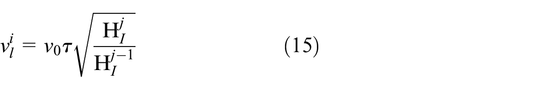
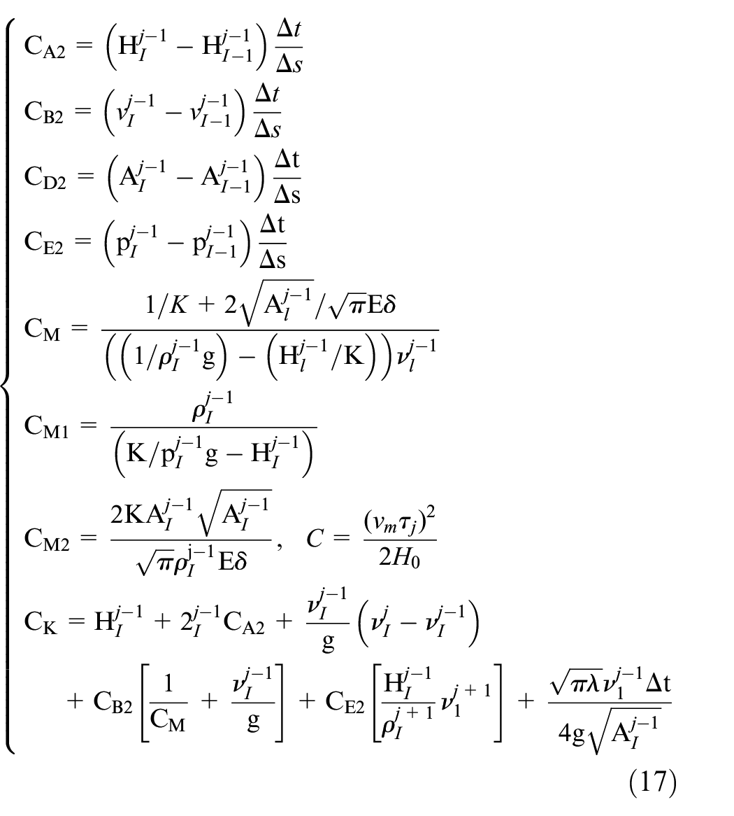
The equations (15) and (5) are combined to obtain the fluid velocity, pressure head, fluid density and cross-sectional area of the pipeline at any time at the end of the pipeline:

$$\{\begin{array}{c}{H}_I^j=-\frac{{\mathrm{v}}_{\mathrm{I}}^{\mathrm{j}-1}}{\mathrm{g}}{\mathrm{v}}_{\mathrm{I}}^{\mathrm{j}}+{\mathrm{C}}_{\mathrm{K}}\hfill \\ {\nu }_I^j=-\frac{{\nu }_I^{j-1}}{\mathrm{g}}\mathrm{C}+\sqrt{{\left(\frac{{\nu }_I^{j-1}\mathrm{g}}{\mathrm{C}}\right)}^2-2\mathrm{C}{\mathrm{C}}_{\mathrm{K}}}\hfill \\ {\rho }_I^j={\rho }_I^{j-1}-{\nu }_I^{j-1}{C}_{\mathrm{E}}+C_{\mathrm{M}1}(H_I^j-H_I^{j-1}+{\nu }_I^{j-1}{C}_{\mathrm{A}2})\hfill \\ A_I^j=A_I^{j-1}-C_{\mathrm{D}2}{\nu }_I^{j-1}+C_{\mathrm{M}1}{C}_{\mathrm{M}2}(H_I^j-H_I^{j-1}+{\nu }_I^{j-1}{C}_{\mathrm{A}2})\hfill \end{array}$$

(16)

$$\{\begin{array}{c}{\mathrm{C}}_{\mathrm{A}2}=({\mathrm{H}}_I^{j-1}-{\mathrm{H}}_{I-1}^{j-1})\frac{\mathrm{\Delta }t}{\mathrm{\Delta }s}\hfill \\ {\mathrm{C}}_{\mathrm{B}2}=(v_I^{j-1}-v_{I-1}^{j-1})\frac{\mathrm{\Delta }t}{\mathrm{\Delta }s}\hfill \\ {\mathrm{C}}_{\mathrm{D}2}=({\mathrm{A}}_I^{j-1}-{\mathrm{A}}_{I-1}^{j-1})\frac{\mathrm{\Delta }\mathrm{t}}{\mathrm{\Delta }\mathrm{s}}\hfill \\ {\mathrm{C}}_{\mathrm{E}2}=({\mathrm{p}}_I^{j-1}-{\mathrm{p}}_{I-1}^{j-1})\frac{\mathrm{\Delta }\mathrm{t}}{\mathrm{\Delta }\mathrm{s}}\hfill \\ {\mathrm{C}}_{\mathrm{M}}=\frac{1/K+2\sqrt{{\mathrm{A}}_l^{j-1}}/\sqrt{\pi }\mathrm{E}\delta }{((1/{\rho }_I^{j-1}\mathrm{g})-({\mathrm{H}}_l^{j-1}/\mathrm{K})){\nu }_l^{j-1}}\hfill \\ {\mathrm{C}}_{\mathrm{M}1}=\frac{{\rho }_I^{j-1}}{(\mathrm{K}/{\mathrm{p}}_I^{j-1}\mathrm{g}-{\mathrm{H}}_I^{j-1})}\hfill \\ {\mathrm{C}}_{\mathrm{M}2}=\frac{2{\mathrm{KA}}_I^{j-1}\sqrt{{\mathrm{A}}_I^{j-1}}}{\sqrt{\pi }{\rho }_I^{\mathrm{j}-1}\mathrm{E}\delta },C=\frac{{(v_m{\tau }_j)}^2}{2H_0}\hfill \\ {\mathrm{C}}_{\mathrm{K}}={\mathrm{H}}_I^{j-1}+2_I^{j-1}{\mathrm{C}}_{\mathrm{A}2}+\frac{{\nu }_I^{j-1}}{\mathrm{g}}({\nu }_I^j-{\nu }_I^{j-1})\hfill \\ +{\mathrm{C}}_{\mathrm{B}2}[\frac{1}{{\mathrm{C}}_{\mathrm{M}}}+\frac{{\nu }_I^{j-1}}{\mathrm{g}}]+{\mathrm{C}}_{\mathrm{E}2}\left[\frac{{\mathrm{H}}_I^{j-1}}{{\rho }_I^{j+1}}{\nu }_1^{j+1}\right]+\frac{\sqrt{\pi \lambda }{\nu }_1^{j-1}\mathrm{\Delta }\mathrm{t}}{4\mathrm{g}\sqrt{{\mathrm{A}}_I^{j-1}}}\hfill \end{array}$$

(17)

Although the running pump generates pressure fluctuations, a pulsation attenuator was installed between the pump and the measurement pipeline in this study to dampen the pump-induced pressure pulsations. The inlet of the measurement pipeline is defined as the interface between the pulsation attenuator and the measurement pipeline. Therefore, in the calculation of water hammer pressure pulsation, the pressure head change at $H_0^j$ is very small and can usually be ignored, that is, $\partial H_0^j/\partial t=0$ . The equations of motion, fluid elasticity and pipeline elasticity are combined to obtain the pressure head, fluid velocity, fluid density and pipeline section at any time at the entrance of the pipeline, as shown in equation (18).

When the initial state of the valve port is closed, this model can still be used to solve and predict, the only difference being that equation (11) determines the change in state.

$$\{\begin{array}{c}{\mathrm{H}}_0^j={\mathrm{H}}_0\hfill \\ v_0^j=v_0^{j-1}(1-{\mathrm{C}}_{\mathrm{B}2})-\mathrm{g}({\mathrm{C}}_{\mathrm{A}2}+({\mathrm{H}}_0^{j-1}/{\rho }_0^{j-1}){\mathrm{C}}_{\mathrm{E}2}\hfill \\ +\sqrt{\pi }\lambda v_0^{j-1}\left|v_0^{j-1}\right|/4\sqrt{{\mathrm{A}}_0^j})\hfill \\ {\rho }_0^j={\rho }_0^{j-1}-v_0^{j-1}{C}_{\mathrm{E}2}+C_{\mathrm{M}1}{v}_0^{j-1}{C}_{\mathrm{A}2}\hfill \\ {\mathrm{A}}_0^j{=\mathrm{A}}_0^{j-1}-v_0^{j-1}{\mathrm{C}}_{\mathrm{D}2}+{\mathrm{C}}_{\mathrm{M}1}{\mathrm{C}}_{\mathrm{M}2}{v}_0^{j-1}{\mathrm{C}}_{\mathrm{A}2}\hfill \end{array}$$

(18)

$$\{\begin{array}{l}{\mathrm{C}}_{\mathrm{A}2}=({\mathrm{H}}_1^{j-1}-{\mathrm{H}}_0^{j-1})\frac{\mathrm{\Delta }\mathrm{t}}{\mathrm{\Delta }\mathrm{s}},{\mathrm{C}}_{\mathrm{B}2}=({\mathrm{v}}_1^{j-1}-{\mathrm{v}}_0^{j-1})\frac{\mathrm{\Delta }\mathrm{t}}{\mathrm{\Delta }\mathrm{s}}\\ C_{\mathrm{D}2}=({\mathrm{A}}_1^{j-1}-{\mathrm{A}}_0^{j-1})\frac{\mathrm{\Delta }\mathrm{t}}{\mathrm{\Delta }\mathrm{s}},C_{\mathrm{E}2}=({\rho }_1^{j-1}-{\rho }_0^{j-1})\frac{\mathrm{\Delta }\mathrm{t}}{\mathrm{\Delta }\mathrm{s}}\\ C_{\mathrm{Ml}}=\frac{p_0^{j-1}}{\left(\mathrm{K}/p_0^{j-1}\mathrm{g}-{\mathrm{H}}_0^{j-1}\right)},C_{\mathrm{M}2}=\frac{2{\mathrm{KA}}_0^{j-1}\sqrt{A_0^{j-1}}}{\sqrt{\pi }{\rho }_0^{j-1}\mathrm{E}\delta }\end{array}$$

(19)

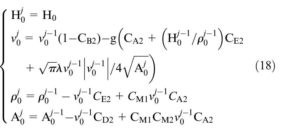
The solution process of the water hammer model is shown in Figure 7. The computational procedure in Figure 7 is as follows: (1) Set the initial parameters at time zero based on the hydraulic system structure. (2) Calculate the pressure at any internal pipe node at any time using equations (8) and (9). This involves: (a) First executing equation (9). (b) Then sequentially calculating H, V, ρ and A from equation (8). (3) Solve for the pressure at the pipe’s initial position and end position using equations (16)–(19). During this step, the valve opening variation is continuously monitored via equation (11) to ensure solutions for equations (18) and (19) are obtained under any driving frequency. (4) Output the results once the computation runs for the specified total simulation time.

Figure 7.

Water hammer pressure calculation flow chart.

Test-bed design

The designed water hammer pressure pulsation test bench includes three parts: drive control system, data acquisition system and hydraulic system. The drive control system mainly writes the program into the Arduino control board through the upper computer and then sends the drive command to the high-speed switch valve through the drive board to realize the switch frequency control.

The structure is shown in Figure 8(a). The data acquisition system is mainly designed based on LabVIEW software platform. It can classify the signals collected by various sensors through NI acquisition card, display them in real time, and realize the functions of data storage. Ensure that the relief valve remains closed throughout the entire experiment to minimize its interference with pressure measurements. The structure is shown in Figure 8(b). The hydraulic system is mainly composed of pump station, control cabinet, various sensors and pipelines, as shown in Figure 8(c). The parameters of the key components of the test bench are shown in Table 1.

Figure 8.

Test bench structure diagram. (a) Schematic diagram of the test bench. 1 – Oil filter; 2 – Hydraulic pump; 3 – Motor; 4 – Pressure oil filter; 5 – Relief valve ; 6 – Pressure sensor; 7 – High-speed on-off valve; 8 – Flowmeter; 9 – Load valve; 10 – Cooler; 11 – Oil filter; 12 – Fuel tank. (b) Drive control system. (c) Data acquisition system. (d) Water hammer pressure pulsation hydraulic test platform.

Table 1.

Key component parameters in the test bench.

Parameter	Numerical value
Rated pressure of hydraulic pump	35 MPa
Displacement of hydraulic pump	8 mL/r
Maximum range of pressure sensor	40 MPa
Accuracy of pressure sensor	±0.1% FSO
Response time of pressure sensor	<0.5 ms
Natural frequencies of pressure sensor	30 kHz
Maximum range of flowmeter	16 L/min
Natural frequencies of flowmeter	1000 Hz
Reproducibility of flowmeter (measured value)	±0.1%
Temperature	35°C(±2°C)
Pipe elevation	0.5 m
Natural frequencies of the pipeline system	80 Hz
Pipeline materials	Steel wire braided hose
Response time of valve	0.5 ms
The highest frequency of the valve	600 Hz
Valve driving voltage	24 V

Test-bed design

Time domain analysis

The water hammer pressure pulsation of digital hydraulic system is simulated and analyzed by using a new model which can solve the water hammer pressure pulsation under continuous on/off. At the same time, the simulation results are verified by the designed water hammer pressure pulsation test bench. In addition, through simulation and experimental data, the changes of water hammer pressure at different switching frequencies are also analyzed. The model parameters are defined as presented in Table 2.

Table 2.

Model parameter settings.

Parameter	Numerical value
Pipe length	1.3 m
Frictional loss factor	0.042
Bore of pipe	0.16 m
Pipe wall	0.025 m
Stable pressure of pump source	8 × 106 Pa
Effective closing time	0.5 ms
Elastic modulus of pipes	1 × 1011 Pa
Fluid modulus	1.32 × 109 Pa
Fluid density	862 kg/m3
Kinematic viscosity	34.4 mm2/s
Acceleration of gravity	9.8 m/s2
Pressure wave velocity	$\sqrt{K/\rho }/\sqrt{1+\mathrm{KD}/E\delta }$
Effective opening time of valve port	0.5 ms

Using the data from Table 2, both the traditional water hammer model and the new water hammer model are employed to analyze water hammer pressures at various switching frequencies. The differences between their results are compared. Additionally, the water hammer pressure pulsations obtained from both models are compared with experimental data measured from the test bench. Figure 9 illustrates the comparison between the traditional and new water hammer models, along with the water hammer pressure pulsations at different on/off frequencies.

Figure 9.

Comparison of experimental models of water hammer pressure at different frequencies. (a) Analysis of water hammer pressure fluctuation of experiment and new model at 10 Hz. (b) Analysis of water hammer pressure pulsation in the experiment and the original model at 10 Hz. (c) Analysis of water hammer pressure fluctuation of experiment and new model at 50 Hz. (d) Analysis of water hammer pressure pulsation in the experiment and the original model at 50 Hz. (e) Analysis of water hammer pressure fluctuation of experiment and new model at 90 Hz. (f) Analysis of water hammer pressure pulsation in the experiment and the original model at 90 Hz. (g) Analysis of water hammer pressure fluctuation of experiment and new model at 150 Hz. (h) Analysis of water hammer pressure pulsation in the experiment and the original model at 150 Hz.

The curve changes in Figure 9 indicate that as the on/off frequency increases, the waveform of the water hammer pressure wave gradually becomes monotonous. The curve changes in Figure 8 indicate that as the on/off frequency increases, the waveform of the water hammer pressure wave gradually becomes single. In Figure 9(a) and (b), it is evident that at a frequency of 10 Hz, there is a momentary damped oscillation in the water hammer pressure wave. Conversely, in Figure 9(e) and (f), at a frequency of 90 Hz, the damped oscillation in the water hammer pressure wave has ceased. Therefore, the frequency of the valve will affect the pressure wave attenuation oscillation. In Figure 9(c), (e) and (g), the changes of pressure pulsation at different frequencies are described in three ways: original model, ²⁸ new model (i.e. the water hammer prediction model established in this article.) and experiment.

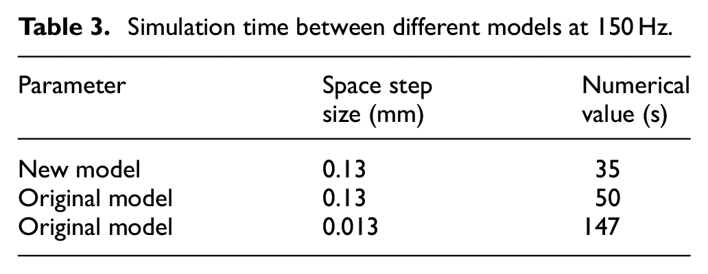
From the curve change, it is found that under the same spatial step size setting, with the increase of frequency, the calculation accuracy of the traditional water hammer model gradually decreases, and the calculation does not converge. Only by improving the accuracy of the spatial step size of the original model, can the convergence calculation be realized. As seen in Figure 9(h), although the original model can improve simulation accuracy by reducing the spatial step size, its computation time is significantly increased, reaching 147 s (see Table 3). Table 3 also reveals that the computation time of the new model under the same temporal step size is less than that of the original model. This difference arises because the original model inherently lacks the capability to predict and evaluate water hammer pressure waves generated by continuous valve on/off. In this study, the data for the original model were obtained by superimposing multiple pressure waves based on the principle of wave interference. This superposition process necessitates multiple computational cycles, leading to increased computation time. Furthermore, reducing the spatial step size increases the model’s computation time due to the fixed relationship between spatial and temporal step sizes (Δl = c × Δt). When the spatial step size decreases, the temporal step size must also decrease. This results in a substantial increase in grid density throughout the computation domain, consequently causing a significant increase in computation time.

Table 3.

Simulation time between different models at 150 Hz.

Parameter	Space step size (mm)	Numerical value (s)
New model	0.13	35
Original model	0.13	50
Original model	0.013	147

In addition, it is also found in Figure 9 that the period of the water hammer pressure wave generated in the digital hydraulic system is always consistent with the switching period of the valve port. In Figure 9(a), a complete water hammer pressure change curve is taken for analysis. It is found that the calculation results of the new model are more accurate than the original model, indicating that the new model is more suitable for calculating the interference between multiple water hammer pressure waves.

Figure 10 illustrates how varying the valve’s frequency affects water hammer pressure fluctuations across different systems. Specifically, Figure 10(a) depicts the amplitude variations of water hammer pressure fluctuations at on/off frequencies of 8, 6, 4 and 2 MPa. Since the original model obtains some non-physical solutions under the same step size setting, the calculation results of the original model are not compared with other results in Figure 8. The data changes described in Figure 10(a) are obtained under the settings of System 1, which is parameterized as shown in Table 1. Thus, from Figure 10(a), it is observed that as the frequency increases, the amplitude of water hammer pressure first increases and then decreases. By comparing the pressure fluctuation curves obtained from experiments and those predicted by the new model in Figures 9 and 10, it is evident that they exhibit a high degree of similarity in waveform, periodicity and amplitude changes of the water hammer pressure wave. This provides strong evidence supporting the accuracy of calculations in the new water hammer model. To validate the universality of the new model and the newly discovered phenomena, a redesigned test system (System 2) was implemented. Key parameters were adjusted: the pipeline length was set to 3 m, the inner diameter to 19 mm and the pipe wall to 5 mm. System 2 was used to analyze the impact of varying frequencies on water hammer pressure fluctuation amplitudes at 4 MPa. The findings are depicted in Figure 9(b). The variation trend of pressure amplitude is consistent with the results obtained by system 1. Therefore, this result once again proves the accuracy of the model, and also proves the universality of the new phenomena found.

Figure 10.

Variation of water hammer pressure with frequency in different digital hydraulic systems. (a) The fluctuation of water hammer pressure at different frequencies in digital hydraulic system 1. (b) The fluctuation of water hammer pressure at different frequencies in digital hydraulic system 2.

To delve deeper into the relationship between the switching frequency of the on-off valve and water hammer pressure pulsations in the digital hydraulic system, the time-domain data underwent Fourier transformation. This process enabled the extraction of spectra depicting water hammer pressure pulsations at varying frequencies. This section primarily centers on the water hammer pressure pulsation data collected from the pressure pulsation test bench and compares it with results generated by the new model under a pump source pressure of 8 MPa. Figure 11 illustrates the spectrum of water hammer pressure fluctuations at various frequencies under this condition.

Figure 11.

Spectrum of water hammer pressure fluctuation at different switching frequencies. (a) Spectrum analysis of water hammer pressure pulsation at 10 Hz. (b) Spectrum analysis of water hammer pressure pulsation at 50 Hz. (c) Spectrum analysis of water hammer pressure pulsation at 90 Hz. (d) Spectrum analysis of water hammer pressure pulsation at 150 Hz.

As depicted in Figure 11, the period of pressure pulsations in the digital hydraulic system changes in accordance with the on/off frequency of the valve port, aligning closely with the switching frequency. Additionally, a comparison between experimental and simulated water hammer pressure pulsations reveals that the simulation exhibits more pronounced high-frequency pressure pulsations compared to those observed in experiments. The reason for this phenomenon is that only steady-state friction is considered in the simulation. ³⁴ It can be seen from Figure 11(c) and (d) that there are no other pressure waves when the on/off frequency exceeds 90 Hz, which is obviously inconsistent with the actual situation. It is proved that the original model cannot accurately analyze the water hammer pressure under continuous on/off, especially when the valve on/off frequency is high.

In the original model, the spectrum plots of Figure 11(c) and (d) show almost no amplitude beyond the valve opening/closing frequency. This is because the original model cannot predict or evaluate the water hammer pressure pulsations generated by continuous valve operations. To enable the original model to analyze water hammer pressure pulsations caused by sustained valve opening/closing, this study adopts a superposition method based on multiple water hammer pressure waves generated by single valve actuations. Consequently, as the frequency increases, the attenuation time of pressure waves decreases. When the frequency reaches a certain threshold, the water hammer pressure waves lose their attenuation process, resulting in simplified waveforms.

When Figure 11 is combined with Figure 10, it can be observed that the frequency of the water hammer pressure wave is more prominent at 90 Hz. The reason for this phenomenon is that at this frequency, the valve on/off frequency coincides with the inherent water hammer cycle of the system, resulting in resonance. The inherent water hammer period of the system can be solved according to Wang et al. ³⁵

Conclusion

This paper explores the water hammer pressure pulsations caused by high-speed on-off valves in digital hydraulics. A dedicated water hammer pressure pulsation test bench was designed for this investigation. This study determined the relationship between the on/off frequency of valves in digital hydraulic valve control systems and the resulting water hammer pressure pulsation:

• (1) The main frequency of the water hammer pressure wave varies in accordance with changes in the switching frequency of the valve, demonstrating a consistent relationship with the on/off frequency.

• (2) The amplitude of pressure waves in digital hydraulic valve control systems shows a trend of first increasing and then decreasing with the increase of valve on/off frequency. When the on/off frequency is equal to the inherent water hammer frequency of the digital hydraulic system, the pressure pulsation amplitude reaches its maximum value.

• (3) The waveform of the water hammer pressure wave gradually becomes monotonous as the on/off frequency increases. At lower on/off frequencies, the waveform exhibits a process of attenuated oscillations in water hammer pressure. As the frequency increases, the time of attenuation oscillation in the waveform gradually shortens until it disappears.

In order to achieve theoretical analysis of switch frequency and water hammer pressure pulsation, a function of valve opening variation with time was constructed, and a water hammer model that can calculate continuous switching was established. Experimental verification confirmed the accuracy of the new model. This model addresses the limitations of existing models in describing the new phenomenon, thereby enhancing the accuracy of water hammer model prediction and analysis. Furthermore, the newly established model achieves an amplitude error not exceeding 5% when predicting water hammer pressure pulsations generated by the continuous switching of high-speed valves. This has laid a solid foundation for further accurate analysis of the impact of pulsating fluids on pipeline systems, and provided theoretical guidance for the design of high reliability and low vibration digital hydraulic systems.