
Abstract
Test benches are useful tools for testing bogies in laboratory conditions, most of which consist of large rollers to move the wheels of the bogies, either at a reduced scale or at full size. The full-scale test rig located at the BOGLAB laboratory uses two small rollers to move each wheel of one of the bogie’s wheelsets. This paper presents a 21-DOF dynamic model of a two-axle bogie running on this double roller test rig that considers the motion of the two wheelsets, the bogie frame and the four axle boxes, which is not usually implemented in the models of the literature. The model also computes the creepages, creep and normal forces originating from the contact of the two rollers on each wheel. The simulation results show the movement transmission from the front wheelset to the rear wheelset due to the specific configuration of this test bench. A sensitivity analysis is performed to study the influence of bogie load and speed on the vertical acceleration of the axle boxes. Data show that increasing the bogie load leads to higher vertical acceleration in the axleboxes. The effect of speed is nonlinear, revealing a threshold speed beyond which vertical accelerations significantly decrease.
Introduction
In 2015, the United Nations adopted the 2030 Agenda for Sustainable Development and its 17 Sustainable Development Goals (SDGs) to promise a healthier planet and secure the rights and well-being of everyone on Earth. Railways can play a relevant role in achieving the SDGs, as it is a very efficient transport method that can help reduce pollution and energy consumption in the movement of people and goods.
Maintenance is a key aspect of keeping the efficiency and safety standards of railways and thereby contributing to the achievement of the SDGs. However, predictive maintenance requires extensive knowledge of the rolling stock to determine the best time to perform the maintenance tasks. In this sense, mathematical models of rolling stock offer a good approach, as they allow studying the performance of rolling stock in different conditions and at lower costs than experimental testing with real vehicles.
Lots of models can be found in the scientific literature,1–9 most of them focused on the stability of the railway vehicle. For example, Lee and Cheng use a linearised bogie model to investigate the influence of several parameters on the bogie’s performance in straight 10 and curved tracks. 11 Song et al. 12 introduce a distributed masses model to control the stability of a high-speed train. This is achieved by moving two actuators placed transversely in both bogie ends. The system is tested in a 1:5 scale bogie test rig. Bosso et al. 13 present a bi-dimensional model of the friction dampers used in the Y-25 freight bogie. Then, stability analyses are performed. Molatefi et al. 8 proposes a mathematical model for studying the stability of a freight wagon. This model includes several non-linear phenomena such as non-linear springs and clearances. Shin et al. 14 use a dynamic model implemented in Simpack to develop an algorithm able to detect hunting instability from acceleration signals. All these works focus on the stability of rail vehicles but don’t take into account the effect of external excitations like, for example, track irregularities.
Among the models that also consider the influence of vibrations in the dynamic behaviour of the rolling stock, the following can be highlighted. Demir 15 develops a multibody model of a rapid transit vehicle with several degrees of freedom. Then, track irregularities are simulated according to the standards and the suspension parameters are characterised so that the measured vibration is within the standard margins. True et al. 16 use the model developed in previous works 17 to attempt to detect the track geometry from the dynamic reactions measured in the wheelset. Lebel et al. 18 use Bayesian methods for monitoring the suspension health condition based on acceleration data. Dumitriu 19 uses rail vehicle models that combine rigid and flexible solids to establish the operating condition of primary suspension dampers. Simulation results are combined with vibration data measured in the actual vehicle. Bernal et al. 20 present a bogie model to detect the wheel flat from the accelerations measured in the wheelset, the bogie and the wagon. The model is implemented in GENSYS and compared to previous works, obtaining similar results. These authors also 21 propose a quarter-vehicle model to estimate the characteristics of a low-cost system that detects wheel flats. This system is subsequently tested on a 1:4 scale test bench.
Nevertheless, the number of works that focus on simulating the behaviour of a bogie in a roller test rig is limited. Iwnicki and Wickens 22 proposed the dynamic model of a 1:5 scale bogie running on a test rig. Each wheel of the bogie is moved by a large roller (in relation to the wheel radius). Later, Liang et al. 23 developed a two-degree-of-freedom model of this scaled bogie to study wheel flats and rail defects. The acceleration measured in the axle box of a scale bogie is the input of the mathematical model. Liu et al. 24 propose a dynamic model of a test rig. The system consists of two rollers of large diameter, the wheelset and the primary suspension of the bogie. The model is used to investigate the relationship between defects in the wheel and/or rail and the vibrations registered in the gearbox attached to the axle. Shrestha et al. 25 compare the performance of a scaled bogie roller test rig with de numerical model developed in GENSYS.
As Myamlin et al. 26 expound, the majority of roller test rigs use a large roller to induce the motion of the wheelset (or wheel in some cases), which is the case of the aforementioned studies. However, BOGLAB has a full-scale bogie test bench that uses two small rollers to move one of the wheelsets of the bogie. A system that is not found in the examined scientific literature. This kind of test bench derives from the underfloor wheel lathes used for wheel reprofiling and has the advantage of not requiring an auxiliary structure for keeping the bogie or rail vehicle correctly positioned on the test bench. For geometric and dynamic reasons, placing two cylinders one on top of the other leads to an unstable position, as the upper cylinder will tend to roll over the lower one and fall. Therefore, single-roller test stands have an auxiliary structure to hold the bogie or wheelset in its proper position. This is unnecessary on two-roller test benches, as the geometry of the test bench allows the wheelsets to be supported without external support. However, two-roller test benches have two major disadvantages. By using small-diameter rollers, the contact pressures are higher, and there are two points of contact instead of just one. In addition, this configuration completely changes the running behaviour of the wheelset.
In essence, the reviewed scientific literature can be classified into three groups according to the main topic of the works:
Development of dynamic models for studying the stability of rail vehicles on tracks without including irregularities or defects.1–14
Dynamic models that include any kind of defects or irregularities to analyse their impact on the vehicle’s behaviour.15–21
Simulation of the performance of rail vehicles on a one-roller test rig, usually at scales 1:4 and 1:5,22–25 and occasionally study of defects.
It is extremely rare to find dynamic models that consider axle boxes, though this is the typical place to install the accelerometers when measuring the performance of actual rail vehicles.
The authors propose a bogie model to simulate the performance of a freight bogie tested in a double roller test rig. This model considers the bogie frame, the wheelsets and the axle boxes, as well as the contact between the two rollers of the test rig and the wheel. Therefore, this paper introduces two key innovations to the scientific community. Firstly, it considers the axle boxes in the model, which are not usually taken into account in scientific literature, and paves the way for roller bearing models to be included in future studies. Secondly, it calculates the contact forces due to the action of two small rollers on a wheel.
The structure of the paper is as follows: the second section describes the bogie under study. The third section expounds the mathematical model of the bogie. The results obtained from the simulation are discussed in the fourth section. Finally, the conclusions are described in the fifth section.
System description
Bogie description
The bogie under study in this work is a freight bogie of type Y-21 Cse, which is based on the Y-25 bogie widely used in Europe for freight wagons. This type of bogie has two wheelsets that can load up to 20 tonnes per axle and is adapted to run on the Spanish rail network, so its track gauge is wider than the standard. The main characteristics of the Y-21 Cse bogie are summarised in Table 1.
Bogie y21 CSE characteristics.

The bogie is modelled in CREO Parametric from technical documentation to obtain certain characteristics that would be difficult to get in other ways. Figure 1 shows this 3D CAD model of the bogie.

CAD model of the Y-21 Cse bogie and the double roller test rig.
Test bench description
The BOGLAB laboratory, placed in one of the Renfe main workshops located in the South of Madrid (Spain), has a bogie test rig specifically designed and manufactured by Dannobat Railway Systems to test bogies under different conditions (see Figure 2). The DTR-25 test rig derives from wheel lathes used for wheel reprofiling and is formed by a bench and a drive system that transmits movement to the wheels of the wheelset by means of two small rollers. These rollers have a diameter of 350 mm, and the contact geometry is the same as the profile of UIC-54 rails. One wheelset (rear) stands over the fixed bed, and the other (front wheelset) is driven by the rollers. The system that drives the rollers allows the simulation of the operating conditions of the front wheelset of the bogie for speeds between 0 and 80 km/h. It is also possible to change the rotating direction of the wheelset, simulating the movement of the bogie forward or backwards. Two of the four rollers are moved by electric traction motors, while the other two rollers are moved by wheel/roller friction. Traction motors are coupled following a master-slave logic.

Installed bogie on the test bench.
The load is applied vertically thanks to a hydraulic system. This system consists of a couple of hydraulic cylinders that pull a horizontal beam placed above the front axle by using two chains. The maximum bogie load provided by the hydraulic loading system is 20 tonnes.
The geometry of the bogie test rig can support the bogie without the need for external structures, which allows the free movement of the bogie in the vertical and lateral directions, and also some movement in the longitudinal direction. This is an advantage over one roller test rigs, which require a structural support or coupler to maintain the wheel/bogie/vehicle in position.
Having two small rollers, the wheel has at least two contact points at all times, which is a disadvantage if the research aims to study the contact between the wheel and rollers in similar conditions to a tangent track. This configuration results in reduced contact areas and elevated contact pressures, which may lead to accelerated wheel wear if this device were employed in wear simulation applications.
The test rig allows for experiments to be carried out, among others, to analyse the vertical dynamics of the bogie, the performance of the suspension elements or the effect of the presence of defects in components such as rolling bearings, axles, gearboxes, etc. Although the contact conditions differ from those found on track, this type of test rig offers a platform for fatigue testing, the simulation of axle cracks 27 and for studying the behaviour of the bogie on wheel lathes. To extrapolate the results of the test bench to reality, a correlation should be established between the data, which is beyond the scope of this work.
Mathematical model
A 21-degree-of-freedom model is proposed for simulating the behaviour of the Y-21 bogie over the double roller test bench. The model comprises the bogie frame, the two wheelsets and the four axle boxes. The scheme of this model is summarised in Figure 3. As can be seen, the inputs are the bogie load, the speed and the kinematic conditions of the wheels due to the roller and/or wheel irregularities. The outputs are the displacements, velocities and accelerations of the wheelsets, the bogie frame and the axle boxes. The model parameters are the mass and moments of inertia of the bodies, the distances between them and the stiffness and damping coefficients linking all the bodies.

Scheme of model representation.
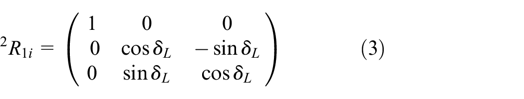
Five coordinate systems are used to establish the dynamics of the wheelset, as can be seen in Figure 4. Coordinate system number 4 is the equilibrium reference frame, which is common to the axle boxes and the bogie frame. The other coordinate systems are obtained by rotating a finite angle about one axis of the previous reference frame. In addition, coordinate systems 0 and 1 are particularised for the front (subscript f) and rear (subscript r) rollers and the left (subscript i) and right (subscript d) wheels, respectively. The coordinate transformation matrices are given by equations (1)–(6), where the left superscript means the destination coordinate system and the right subscript means the origin coordinate system.


Coordinate systems transformation.
Coordinate systems 0 and 1 are related to the contact planes that contain the contact points.

The multibody model developed is shown in Figure 7, where all the bodies and their connections can be observed. Reference frames are placed at the centre of mass of each body. The wheelsets are modelled with four degrees of freedom and can move in the vertical and lateral direction and rotate around the longitudinal (roll) and vertical (yaw) axes. The axle boxes can move in the vertical and axial direction. The bogie frame is allowed to move vertically and laterally and to rotate around the longitudinal (roll), lateral (pitch) and vertical (yaw) axes.

Front view of contact plane axes.

Lateral view of contact plane axes and normal forces.

Two-axle bogie model in front (top) and lateral (bottom) views. For clarity, the rollers have not been drawn in the front view.
The model is developed based on seven subsystems composed of bogie frame (subscript b), forward wheelset (subscript w1), rear wheelset (subscript w2), front left axle box (subscript ab1L), front right axle box (subscript ab1R), rear left axle box (subscript ab2L) and rear right axle box (subscript ab2R). For each subsystem, the classical dynamic equations (Newton’s second law and conservation of angular momentum) are applied in matrix form, as stated in (8) and (9).


Where

In (8) and (9), dots over the vector and variables indicate time differentiation. Variables
Normal contact forces
Hertz’s contact model is used to calculate the shape of the contact area and pressure. The theory predicts the shape of the contact area, its size as a function of the applied normal load N, and the magnitude and distribution of the forces that appear in the contact. The hypotheses on which Hertz’s theory is based are the following28,29:
The surfaces are continuous and non-conformal.
The deformations are small.
Each solid can be considered as an elastic half-space.
There is no friction between the surfaces.
Hertz showed that the contact surface is flat and elliptical, with a major semi-axis
The ratio
The two semi-axes
The penetration
The dimensions of the semi-axes are given by equations (10) and (11).

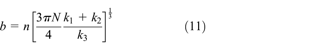


Where:
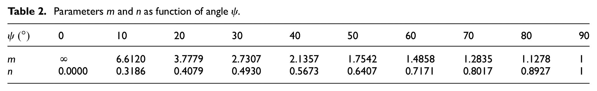
Parameters


Parameters
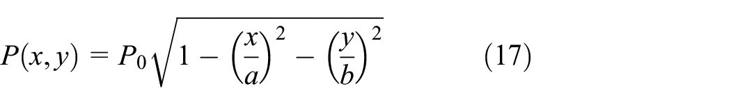
The contact pressure distribution on the contact surface,

Tangential forces
The first step to calculate the tangential forces is to compute the creepages, which are, by definition 29 :


The angular velocity of the wheelset in the coordinates of the wheelset body (CS2) is

The position vectors of the four contact points in terms of the wheelset coordinate system (CS2) are given by equations (23)–(26).


The left superscript refers to the coordinate system, as well as the subscript of the unitary vectors. The subscripts (L, R)(1, 2) refer to the left or right wheel and the front (1) or rear (2) rollers.
In terms of the equilibrium reference frame and using equations (5) and (6), the position vectors are
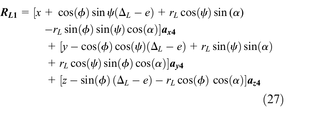
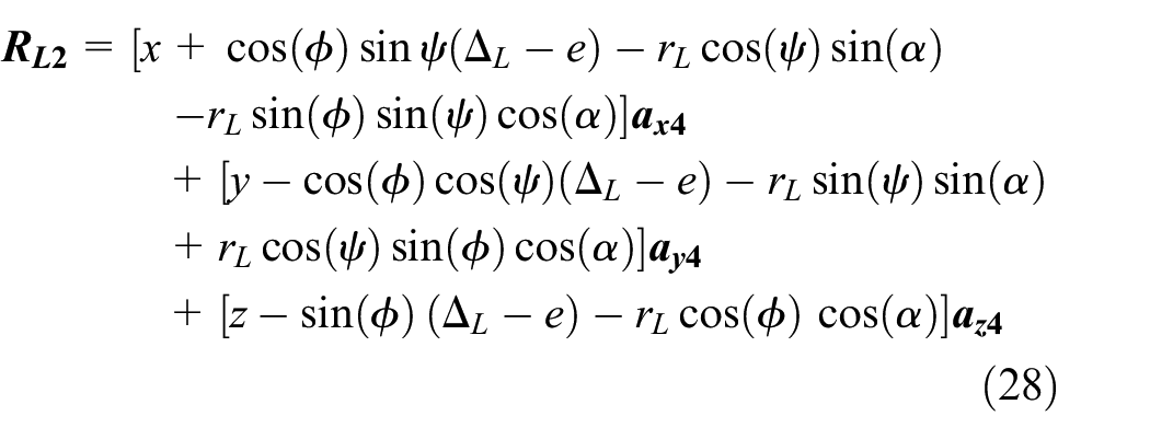


The velocities of the wheels at the contact points are obtained by time-differentiating equations (27)–(30).
The unitary vectors of the contact plane at the contact point between the left wheel and the front left roller in coordinates of the equilibrium reference frame are given by equations (31)–(33).


Similarly, the unitary vectors of the contact plane at the contact point between the left wheel and the rear left roller in coordinates of the equilibrium coordinate system can be obtained using the equations (2), (3), (5) and (6) to get the expressions given by equations (34)–(36).


Equations (37)–(39) define the unitary vectors of the contact plane at the contact point between the right wheel and the front right roller in the coordinates of the equilibrium reference frame.


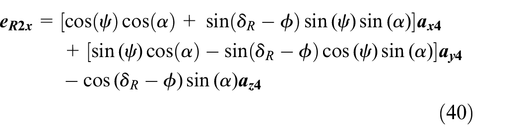
The unitary vectors of the contact plane at the contact point between the right wheel and the right rear roller in coordinates of the equilibrium coordinate system are given by equations (40)–(42).


The velocities of the rollers at the contact points in the coordinates of the equilibrium reference frame are


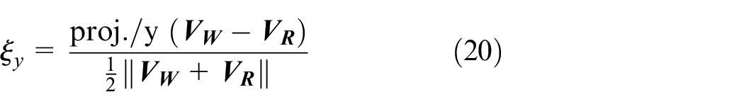
Applying equations (19)–(21) and considering that the projections of the wheel speed to the X and Y axes are


Next, the tangential contact forces are computed using the Fastsim algorithm 30 in the contact plane reference systems. After applying equations (1)–(6) and assuming small angles, the forces are expressed in the equilibrium coordinate system as


Where
By assuming that the displacements

Motion equations
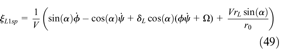
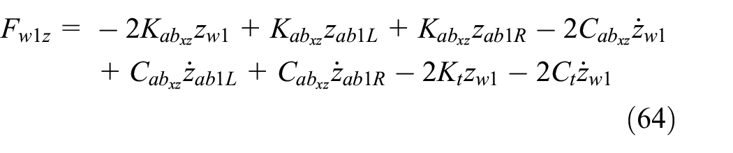
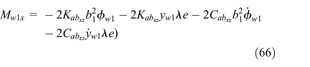
The expressions that describe the suspension forces of the front and rear wheelsets are given by equations (64)–(71). The flexibility of the supports is given by


The flange contact force is given by Ahmadian and Yang 31 as

By combining the suspension forces with the normal and tangential contact forces, the equations of motion of the front wheelset are obtained.
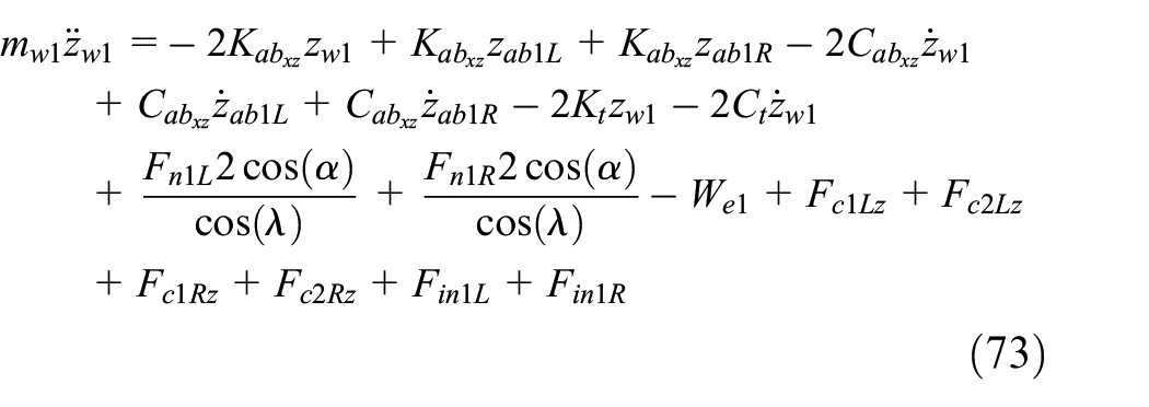
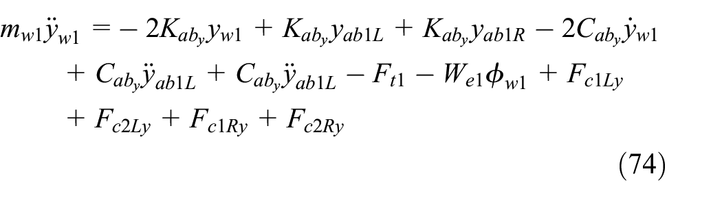
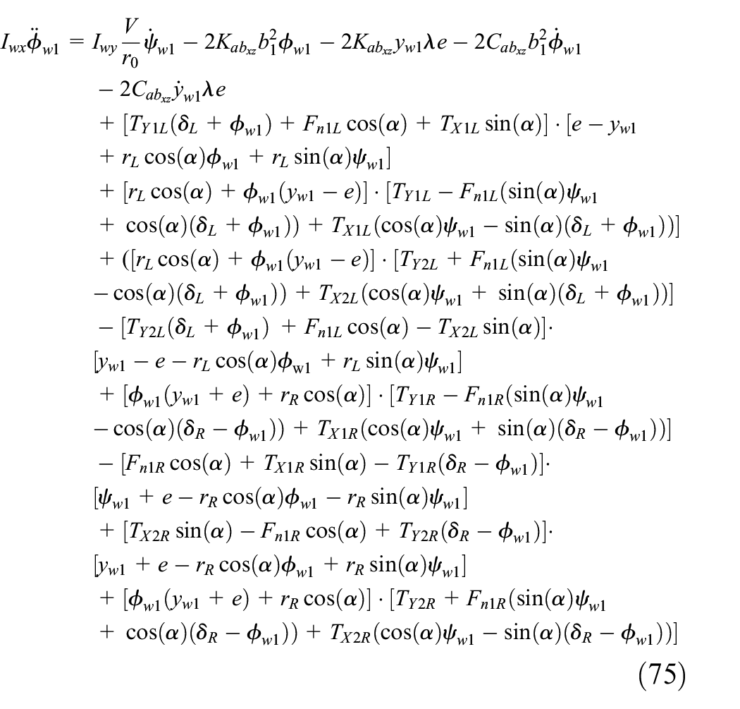

Where
Similarly, the expressions for the motion of the rear wheelset have been defined in (77)–(80), being


The equations that define the motion of the axle boxes are derived from the analysis of the actuating forces on them.


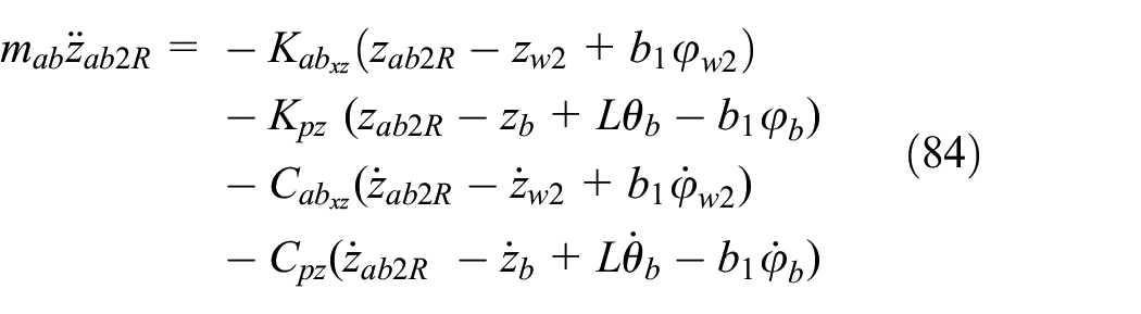


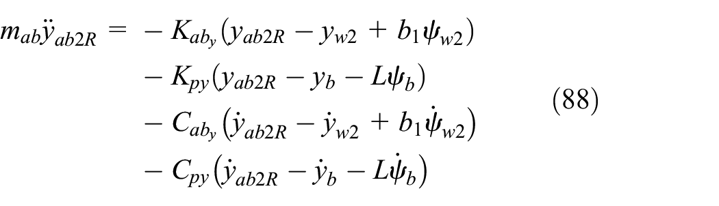
Where
The four equations that define the motion of the bogie frame in the vertical direction and pitch, roll and yaw angles are the following:


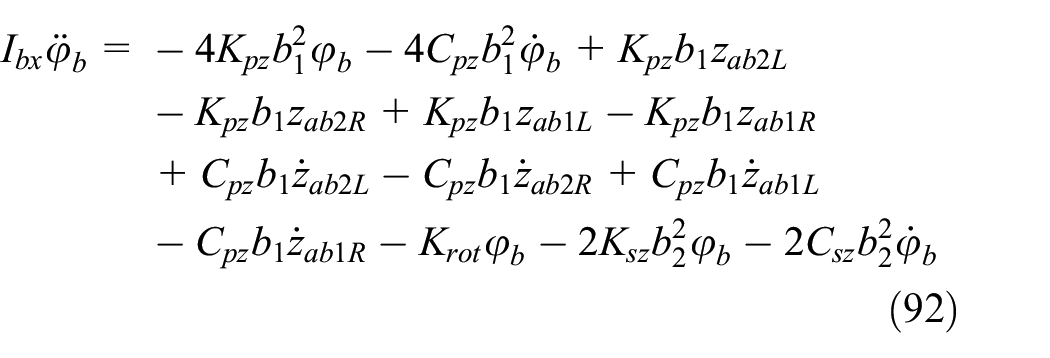

Where
This model is developed for a two-roller test rig, but it can be easily modified to simulate one-roller test rigs by setting the angle
The parameters of the model are listed in Table 3. Mass and inertia data and dimensions are obtained from the 3D CAD model. The stiffnesses and dampings are obtained from technical documentation and other research works 24 or calculated from measurements of the actual bogie.
Model parameters.

Damping on Y-25/Y-21 type bogies is provided by a dry friction-based Lenoir link, which is highly non-linear. Several authors13,32 have proposed different models to simulate the performance of this type of damping. However, computation times become extremely long. This work proposes a linear approach for the damping by setting an equivalent damping based on the research developed by Mazilu and Dinu. 32 The model proposed in this latter work is implemented using our values for the Y-21 bogie and a bogie load of 10 tonnes. The resulting friction force at each time step is divided by the velocity at that time step, giving an equivalent damping as a function of time. Based on these results, the equivalent damping value is chosen, which is represented by the black line of Figure 8.

Friction force computed using Mazilu and Dinu 32 (top) and equivalent damping (bottom).
Simulation results
First, the contact area and pressure distribution are computed, as these data are part of the input to compute the contact forces. Although this work focuses on the behaviour of the bogie on a two-roller test rig, it is interesting to perform a small comparison between the contact parameters in the wheel/rail and wheel/rollers cases. The contact patches are shown in Figure 9 for a bogie load of 10 tonnes (in addition to the weight of the bogie).

Contact patches in wheel/rail (left) and wheel/rollers (right) cases. The bogie load is 10 t.
The first feature to mention is the aspect ratio of the contact ellipse: in the wheel/rail case, the major semi-axis of the ellipse is in the rolling direction, which results in an
Simulation at 50 km/h
The differential equations introduced in the previous section are implemented in MATLAB and solved using the Dormand-Prince pair, which is based on the Runge-Kutta formula.
34
A first set of simulations is performed at 50 km/h and a bogie load of 10 tonnes to study the performance of the bogie in nominal conditions. Simulation time is set to 10 s in order to obtain a stationary response of the system after the initial transient. No external forces due to roller irregularities or other phenomena are considered. Therefore, the model variables
The vertical displacements (and the velocities) of the front and rear wheelsets quickly reach a stable vertical position around zero after the initial conditions to excite the system. The front wheelset presents a small oscillation of amplitude about 0.6 μm, and the rear wheelset presents an oscillation of amplitude about 0.025 μm. Therefore, these small oscillations are negligible. The same behaviour is observed in the vertical motion of the bogie frame.
The angular displacements of the front wheelset are shown in Figure 10. The left-hand plots illustrate the evolution of the roll and yaw angle of the first wheelset throughout the complete simulation. The right-hand plots provide a zoomed view to facilitate a more comprehensive understanding of the movement. It is evident that, owing to the initial conditions, the roll angle of the front wheelset manifests an initial transient, which is subsequently followed by a trend towards zero. Within this trend (Figure 10, upper right), an oscillation about 170 Hz can be observed.

Time evolution of angular variables of wheelset 1. The right plots are zoomed regions of the left ones. V = 50 km/h, W = 10 t.
On the other hand, the yaw angle starts at zero and develops a sustained oscillation of amplitude about 8.4 × 10⁻⁵ rad. The frequency of this oscillation is about 170 Hz, too.
Figure 11 shows the axial and lateral displacements of the wheelsets and bogie. The front wheelset initially experiences a transient period due to the simulation’s initial conditions, after which it begins to trend smoothly towards zero. In contrast, the displacement of the rear wheelset can be considered negligible. Due to lateral friction between the wheel treads and supporting rails, total motion amounts to just 15 μm. The lateral motion of the bogie frame exhibits damped oscillations due to the initial conditions. This oscillation is the result of the model’s internal flexibilities.

Time evolution of the axial displacement of the front wheelset (up), rear wheelset (middle) and bogie frame (bottom). V = 50 km/h, W = 10 t.
Figure 12 illustrates the behaviour of the angular variables of the bogie frame. After the initial transient, the pitch of the bogie frame stabilises around 1.52 × 10⁻⁶ rad. Closer inspection of its behaviour reveals a sustained oscillation with an amplitude of 0.075 μrad, which could be considered negligible. However, it is interesting that a frequency of approximately 170 Hz can also be identified, as well as its second harmonic. The roll angle of the bogie shows a trend towards zero. Again, a closer look at the plot reveals oscillations of frequency about 170 Hz. The yaw angle of the bogie exhibits a very low frequency oscillation with a peak-to-peak amplitude of 3 × 10⁻⁴ rad. However, what appears to be a simple line turns out to be a higher frequency oscillation on closer inspection. Again, the frequency of around 170 Hz observed earlier appears.
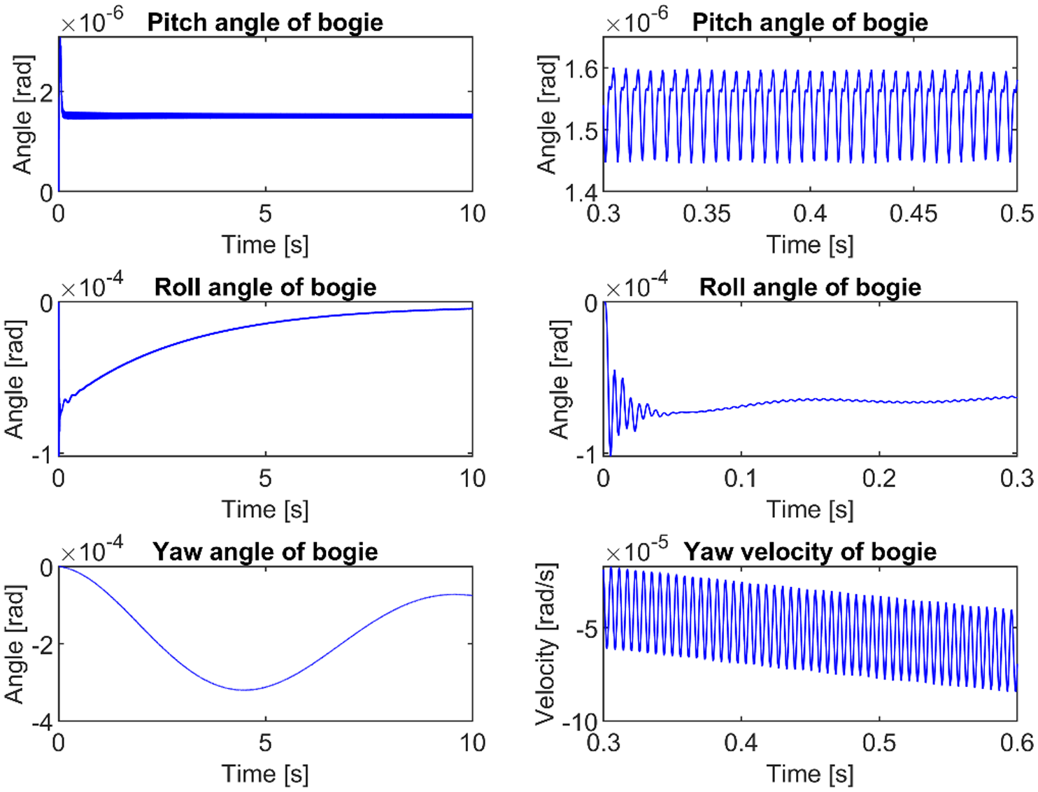
Time evolution of angular variables of the bogie frame. V = 50 km/h, W = 10 t.
As could be expected from the configuration of the test bench, the behaviour of the front and rear axle boxes differs notably in terms of kinematics. These displacements are shown in Figure 13. The front axle boxes follow the same trend as the front wheelset, moving towards zero after the initial transient due to the initial conditions of the simulation. Conversely, the rear axle boxes exhibit damped oscillations for approximately 0.7 s. After this, there is almost no lateral movement of the rear axle boxes: they move laterally by about 12 μm in 9 s.

Time evolution of the axial displacement of the axle boxes. V = 50 km/h, W = 10 t.
As occurs with the wheelsets and the bogie frame, the vertical displacement of the axle boxes is almost imperceptible. However, studying the vertical accelerations reveals interesting features. Due to the initial conditions, the four axle boxes experience vertical accelerations reaching 1.5 × 10⁴ m/s2, which are damped rapidly. Figure 14 shows a zoomed region of the vertical acceleration between 0.3 and 0.5 s. As can be observed from these plots, the vertical acceleration of the front axle boxes oscillates at a frequency of around 170 Hz with an amplitude of around 5 m/s2. As no external periodic forces are applied to the bogie, this phenomenon is due to the model’s internal flexibilities and the contact forces between the wheels and rollers. A similar pattern is evident in the rear axle boxes, though the amplitude of the accelerations is only approximately 0.25 m/s2. As the rear wheelset and axle boxes are only subject to vertical forces from the bogie itself, the vertical movement of the axle boxes results from the transmission of movement from the front wheelset. According to these results, the vertical accelerations registered in the rear axle boxes are about 20 times lower than those registered in the front axle boxes.

Vertical vibrations of the axle boxes (zoomed between 0.3 and 0.5 s). V = 50 km/h, W = 10 t.
To get a comprehensive view of the vertical acceleration of the axle boxes, a frequency analysis is performed. The PSDs of the accelerations are shown in Figure 15. The axle boxes of the front wheelset display a frequency component of high amplitude located at 168.81 Hz, which matches the high-frequency oscillations observed in the previous time plots. The second multiplier of this frequency is also visible at 337.52 Hz. The spectra also show two frequency components whose shape suggests that they are natural frequencies of the system. The first one is located at 162.6 Hz and is almost hidden by the component located at 168.81 Hz. The second frequency is located at around 284 Hz.
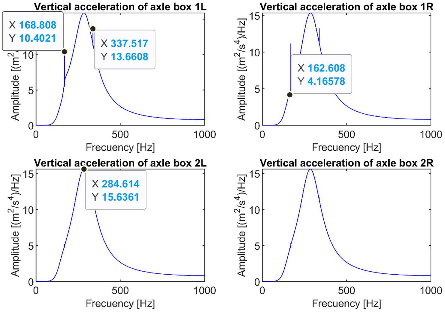
PSD of vertical acceleration of the axle boxes. V = 50 km/h, W = 10 t.
On the other hand, the frequency component of 168.81 Hz and its second harmonic are barely visible in the spectra of the rear axle boxes. The acceleration of these mechanical components is clearly dominated by the frequency around 284 Hz.
Sensitivity analysis
We will focus only on the two parameters that are easily modifiable in the actual test bench: the speed and the bogie load. The bogie load is scanned from 0 tonnes (just the weight of the bogie) to 20 tonnes in steps of 2 tonnes. For each bogie load case, the speed is increased in steps of 5 km/h, starting at 10 km/h up to 130 km/h. As in the previous simulations, no forces from external phenomena are applied.
As sensors for monitoring rolling stock dynamics are typically located in the axle boxes, the sensitivity analysis will focus on the evolution of the RMS acceleration in these four boxes. This parameter can be computed quickly and provides a good indication of the level of vibration experienced by the axle boxes. The results are plotted in Figures 16 and 17.

RMS acceleration of the front axle boxes as a function of speed and bogie load.
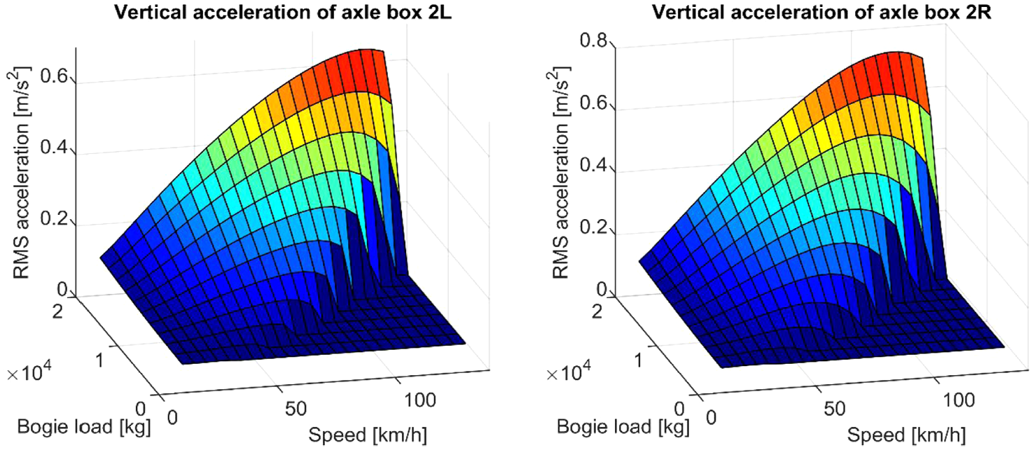
RMS acceleration of the rear axle boxes as a function of speed and bogie load.
The bogie load clearly influences the vertical acceleration of the axle boxes: increasing the bogie load will result in an increase in vertical acceleration at a given speed. However, the effect of speed is more interesting. Increasing speed increases the level of axlebox accelerations, but there is a speed above which vertical accelerations are significantly reduced to the point of being almost imperceptible. The speed at which the trend change occurs depends on the bogie load. For a bogie load of 4 tonnes, this speed is 50 km/h. For 10 and 20 tonnes, this speed increases to 80 and 120 km/h, respectively.
As far as maximum acceleration amplitudes are concerned, the front wheelset axleboxes are in the region of 11 m/s2. The maximum RMS values of the rear axle boxes are around 0.65 m/s2. Therefore, the ratio between the accelerations is somewhat lower than the value of 20 mentioned in the previous section. It should also be noted that the RMS values are slightly higher on the left axle box than on the right axle box in the front wheelset. The opposite occurs in the rear wheelset, where the RMS values are slightly higher on the right axle box than on the left.
Conclusions
A 21-DOF dynamic model of a two-axle bogie is presented in this work. The model considers the vertical and lateral displacements and the roll and yaw angles of the wheelsets, the vertical and lateral displacements of the four axle boxes and the vertical and lateral displacements and pitch, roll and yaw angles of the bogie frame. The inclusion of the axle boxes in the model allows us to simulate the behaviour of this element, which is where vibrations in the rolling stock are usually measured. This element is not usually simulated in the scientific literature and is one of the novelties of this research.
The model is customised to simulate the performance of a Y-21 freight bogie in a two-roller test rig. This type of test rig device rotates one of the wheelsets while the other rests on a fixed rail section. This configuration is typical of wheel lathes and has not been studied in the scientific literature reviewed. The bogie has also been modelled in 3D, so key parameters to characterise the model can easily be extracted. The creepages, creep and normal forces have been calculated taking into account this configuration and introduced into the dynamic model of the bogie. Although this work simulates that specific configuration, any other bogie type can be simulated by just changing the model parameters. In the same way, a test bench that moves the two wheelsets can be simulated by adding the creepages, creep and normal forces to the rear wheelset. One-roller test rigs can be simulated by setting the parameter
A small comparison between the contact surfaces and pressures of the typical wheel/rail contact and this specific wheel/rollers contact case is performed. The results show that the major semi-axis of the contact ellipse changes its direction when the two small rollers are considered. In addition, the contact area is reduced, and the contact pressure is increased. Therefore, the wheels should be subjected to accelerated wear, opening the door to using this type of test rig for studying wheel wear.
The performance of the model is analysed by simulating the behaviour of the bogie at a speed of 50 km/h under a bogie load of 10 tonnes. The lateral friction between the rear wheels and the supporting rail limits the axial movement of the rear wheelset, which induces a yaw movement on the bogie frame as the front wheelset moves laterally from the initial position to centre itself in the longitudinal axis of the bogie. Contact forces between wheels and rollers and internal elements of the system induce vertical vibrations in the system. Front axle boxes are subject to vertical accelerations of amplitude 5 m/s2 that reach the rear axle boxes attenuated around 20 times. The frequency analysis of the vertical acceleration of the axle boxes reveals the existence of a component located at 168.81 Hz and its second multiplier, which explains the high-frequency signals observed in the time domain of certain variables.
A sensitivity analysis is carried out by modifying the two basic parameters that can be changed in the test rig: the speed and the bogie load. According to the results from the simulations, the bogie load has a direct influence on the vertical acceleration of the axle boxes. However, the relationship between the speed and the vertical acceleration of axle boxes is more complicated. The results show that the acceleration increases with speed up to a speed at which the acceleration drops abruptly. In addition, this speed also depends on the bogie load applied.
Future research will focus on experimental validation of the model and simulation of other test setups, including roller bearing models in the axle boxes, as a way to develop a Digital Twin that allows analysing and understanding bogie performance on a test bench for predictive maintenance tasks. However, there is still a long way to go.
Footnotes
Handling Editor: Sharmili Pandian
Funding
The authors disclosed receipt of the following financial support for the research, authorship, and/or publication of this article: The research work described in this paper is part of the R&D and Innovation projects MC4.0 PID2020-116984RB-C21 and MC4.0 PID2020-116984RB-C22 supported by the Spanish Government through MCIN/AEI/10. 13039/501100011033. This publication is part of the R&D Project Intelligent diagnosis of critical railway components, funded by the call ‘Ayudas a Investigadores Tempranos UNED-Santander 2024’.
Declaration of conflicting interests
The authors declared no potential conflicts of interest with respect to the research, authorship, and/or publication of this article.