
Abstract
This paper focuses on the high-precision engineering application of designing and implementing a norm-optimal iterative learning control (ILC) algorithm for the precise positioning of a robotic gripper tip flexibly coupled to an industrial walking beam system. The ILC algorithm generates a feedforward or exogenous signal to minimize tracking errors, thereby enabling high-precision motion control. However, integrating the ILC signal into an existing feedback control system can introduce control signal discontinuities and fluctuations, potentially impairing performance.
To address these challenges, this paper proposes structural adjustments to the feedback control algorithm and the implementation of the ILC signal. The primary objectives are to prevent controller fragility caused by the integration of the ILC signal, ensure stable and feasible dynamics of the control variable, and maintain the desired system performance. This work demonstrates the novel application of norm-optimal ILC to a walking beam system with a flexibly coupled robotic mechanism. To the best of our knowledge, this specific application has not been explored in the literature. Validation through simulations, conducted using a nonlinear plant model in Simscape/Simulink, provides valuable insights into the dynamic behavior and control performance of the system.
Keywords
Introduction
Iterative Learning Control (ILC) is a high-performance control technique tailored for systems executing repetitive tasks. It enhances tracking accuracy by utilizing error information from previous iterations or trials to adjust future control inputs, much like a basketball player improving their free throw through practice.1–3 ILC is particularly effective for systems that demand precise tracking of predefined trajectories, as it progressively reduces tracking errors over successive repetitions.4,5 Moreover, it maintains accurate reference tracking even in the presence of incomplete system models or recurring but unknown disturbances and initial conditions across iterations.1,5
Although the concept of Iterative Learning Control (ILC) is relatively recent, its origins date back to the 1970s.6,7 The first formal and mathematically rigorous study was conducted by Arimoto et al., 8 which is widely regarded as the foundation of ILC research. The first comprehensive book on ILC, authored by Moore, 9 focused on deterministic systems. Thirty years later, Rogers et al. 10 presented an extensive discussion covering ILC applications across linear, nonlinear, distributed, and stochastic systems. For a thorough overview of the fundamental principles, applications, and recent developments in ILC, the review papers2–4,11–13 provide excellent resources.
Based on the literature, three main approaches to synthesizing ILC algorithms are outlined by Matijevic and Kostic 5 : (1) heuristic methods, (2) model inversion-based approaches for feedback systems or controlled subsystems, and (3) optimization-based formulations. Among these, optimization-based designs have demonstrated broad applicability across various domains.14,15 Notable examples include industrial robots, pick-and-place machines, electron microscopes, free-electron lasers, printing systems, wafer stages, healthcare technologies, broiler production systems, quantum control, nuclear fusion, additive manufacturing, and servo systems.
Regardless of the synthesis method, most ILC strategies focus on tracking a reference signal defined over a finite time interval, which is particularly relevant for high-precision engineering tasks. As a result, the spatial tracking problem has also been approached using ILC techniques. However, current implementations of spatial ILC remain highly application-specific, and a general framework applicable across a broader class of systems has yet to be established. 16
In the work of Saab et al., 17 ILC was applied to industrial robot manipulators, with emphasis on challenges related to initial state mismatches and model uncertainties. To address this, a specialized homing controller was introduced to automate state initialization at the end of each iteration. Despite this advancement, transient vibrations were observed, indicating the need for further refinement. Similarly, Yan et al. 18 investigated ILC for robotic manipulators operating under complex initial conditions.
The application of ILC to robotic systems with control variable constraints is addressed in several studies. Meng and He 19 investigated the use of ILC for a robotic arm with input constraints, focusing on vibration suppression and accurate trajectory tracking. Input limitations such as actuator saturation and dead zones can introduce undesirable vibrations, compromising both performance and stability. Chen et al. 20 further explored ILC design under constraints on both control and output variables, demonstrating its effectiveness in maintaining tracking accuracy despite these challenges.
In industrial settings where computational resources are limited, Chi et al. 21 proposed a computationally efficient ILC implementation that avoids matrix inversion. This approach significantly reduces the computational burden, making it practical even for applications with a large number of ILC signal samples.
Meng and He 22 presented an ILC framework aimed at addressing practical implementation challenges in flexible structures, such as vibration suppression, input saturation, dead zones, backlash, external disturbances, and trajectory tracking. The book also introduces simplified partial differential equation models to describe typical problems in flexible structures, which are generally more difficult to stabilize using ILC.
Rogers et al. 10 identified the phenomenon of long-term performance degradation in ILC implementations—a situation where the tracking error initially decreases across iterations but begins to grow again after many trials. This is interpreted as an implementation-related issue rather than a limitation of the theoretical framework.
The design of constrained ILC, including approaches for handling input saturation, is also discussed, notably through the use of receding horizon techniques.
Rogers et al. 23 highlight the numerous opportunities for advancing ILC, particularly in the areas of design, application, and implementation. Persistent challenges—such as actuator saturation, backlash, and integrator windup—underscore the need for continued research to enhance its practical applicability.
This paper investigates the application of norm-optimal ILC to a walking beam motion system featuring a flexibly coupled robotic mechanism. It addresses key implementation challenges and proposes modifications to the control algorithm to enable successful deployment. To the best of our knowledge, the use of norm-optimal ILC in walking beam motion systems has not been reported in existing literature. Related aspects of applying norm-optimal ILC in mechatronic systems with flexible couplings are discussed in References 22, 24–26.
Previous research on walking beam systems has primarily focused on classical control architectures, including PLC-based logic, 27 finite-element-based load simulations, 28 nonlinear model predictive control, 29 and multivariable structure design. 30 These approaches require accurate modeling and often lack adaptability to time-varying system dynamics or unmodeled disturbances. The use of iterative learning control (ILC), especially in its norm-optimal form, has not yet been reported for walking beam applications, despite the method’s proven strengths in repetitive, high-precision motion systems.
Walking beam systems are widely used transfer mechanisms in manufacturing environments, particularly in machining-type transfer lines. 31 They have diverse industrial applications, including bonding machines, metal forming lines, packaging processes that require precise placement, and coordination with pick-and-place units or robotic arms. Their motion is synchronized with upstream and downstream equipment—such as conveyor belts, stamping machines, and robotic grippers—to ensure high throughput and coordinated operation. By synchronously lifting, advancing, and positioning parts across workstations, walking beams enhance automation and productivity.
Over time, these systems have evolved from basic transport components into sophisticated tools for precision motion and assembly tasks. However, achieving both high speed and high positioning accuracy remains a challenge, especially in mitigating vibration. Iterative Learning Control (ILC) addresses these challenges by learning from previous executions to compensate for system uncertainties and improve tracking accuracy. 32 It generates feedforward signals or exogenous inputs that reduce tracking errors, even when system models are incomplete.
Despite these benefits, implementing ILC may lead to abrupt changes in control variables, such as discontinuities or fluctuations, that degrade overall system performance. To mitigate these issues, adjustments to both the control algorithm structure and the implementation of the ILC signals are necessary.
This paper proposes modifications to the norm-optimal ILC algorithm to improve control robustness, ensure smooth control dynamics, and preserve high performance. The proposed method is implemented on a walking beam motion system with a flexibly coupled robotic mechanism. Validation is performed using a nonlinear Simscape/Simulink model that accurately captures multibody dynamics and system nonlinearities.
The model incorporates both feedback and feedforward controllers based on parametric and nonparametric system identification, providing robust control aligned with high-order model behavior. Section “Norm optimal ILC design: Modifications, simulation verification, results, and discussion” presents the ILC algorithm development, simulation setup, and proposed modifications.
For systems with unstable or poorly damped poles, serial norm-optimal ILC architectures are shown to be more suitable than parallel configurations.33,34 The proposed approach addresses issues of controller fragility and excessive control input variations,35–37 enabling stable and efficient system operation. Simulation results in MATLAB/Simulink confirm the effectiveness of the proposed strategy and provide valuable insights into the dynamic behavior of the walking beam motion system.
System description
To highlight its practical relevance, the walking beam motion system analyzed in this paper reflects typical setups found in automated production lines requiring tightly synchronized transfer and placement operations. In general, such a system with a flexibly coupled robotic mechanism is depicted in Figure 1. The control variable is the force F x acting on the walking beam, whose movement is tracked via encoders. The control objective is to ensure that the point of interest (x poi , y poi ) follows a specified reference trajectory. This point corresponds to the tip of the gripper, which is used for high-precision assembly tasks within the machine. Although a sensor to track (x poi , y poi ) during machine operation is unavailable, it is assumed to be present during the development of the control algorithm that generates the control force F x . All parameters shown in the figure are known, enabling the creation of a simulation model of the controlled plant using the Simscape/Simulink module in MATLAB. The gripper is modeled as a thin beam, divided into four finite elements, while the rest of the subsystem is represented by a nonlinear time-invariant model with lumped parameters. Analytical Modeling using Lagrange’s equations and linearization of the nonlinear model is also feasible.
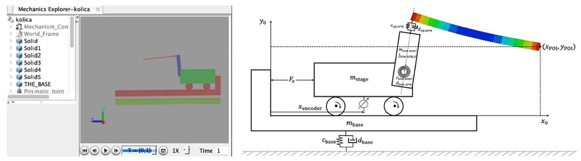
Walking beam motion system with a flexible coupled robotic mechanism.
Based on the known geometric and physical parameters of the rigid bodies and their connections in the multibody system, a software model can be developed in Simscape/Simulink. Linearization or identification techniques can then be applied to this model to derive suitable models for controller design. The Simscape/Simulink simulation model fully corresponds to the controlled plant (or real experimental setup). Figure 2 presents recorded Bode diagrams, serving as nonparametric models of the controlled plant depicted in Figure 1. The parameters listed in Table 1 correspond to a motion system used in industrial wirebonder machines. While the numerical values are not identical to a real wirebonder, the system geometry and the characteristics of the nonparametric model shown in Figure 3—within the desired closed-loop frequency bandwidth—are representative of the actual system.

Simscape/Simulink model of controlled plant from Figure 1, or walking beam motion system with a flexible coupled robotic mechanism.
One example of the possible parameters of the plant from Figure 1.


Nonparametric models of the controlled plant shown on Figure 1.
The Bode diagrams in Figure 3 were generated primarily by estimating frequency response data (FRD models) from simulation-based experiments using broadband noise excitation, including uniform, Gaussian, and PRBS signals. These FRD models formed the core of the analysis and were compared against models obtained through numerical linearization. Coherence functions were computed as well, confirming the reliability of the identification. The resulting FRD models served as the basis for both controller design and performance evaluation.
To ensure reliable excitation across a wide frequency band, all input signals were bounded in amplitude to a maximum of 10 N. The experiments were conducted with a sampling time of T s = 2e-04 s, corresponding to a sampling frequency of 5000 Hz. The PRBS excitation was generated using a 10-bit shift register, yielding a sequence of 210 − 1 = 1023 samples, while white and uniform noise signals provided broadband excitation. In all cases, the usable identification bandwidth ranged approximately from 1 to 400 Hz, which corresponds to roughly twice the expected closed-loop bandwidth of the system.
Walking beam systems are widely deployed in real-world settings where synchronization with adjacent machinery is essential. For example, in metal forming lines, walking beams coordinate with stamping tools and transfer stations to support high-throughput precision manufacturing. In automated packaging, they work in tandem with pick-and-place units to ensure accurate product handling and positioning. These scenarios underscore the practical motivation behind the control strategy developed in this paper.
The structure of the closed-loop system is shown in Figure 4. The feedback loop utilizes the encoder signal to measure the position of the walking beam. The system also includes a feedforward controller,

The coefficients


This formulation ensures smooth and continuous reference signals, along with their first and second derivatives. Although the jerk (third derivative) is not explicitly optimized or constrained, it remains bounded and continuous due to the inherent smoothness of the polynomial. The trajectory is typically extended with idle periods before and after the motion to improve transient handling. This trajectory design inherently limits

Structure of the closed-loop walking beam motion system with integrated feedforward controller.
Consequently, the controller
The feedback controller,
However, achieving the desired motion performance for the walking beam’s position (x) does not necessarily ensure equivalent performance for the point of interest (x poi , y poi ). This point, corresponding to the tip of the gripper, is not rigidly connected to the walking beam motion system. Its motion depends on both the movement of the walking beam and initial conditions, such as the weight of the robotic mechanism’s gripper, the resulting bending effects, and the relative motion between the robotic mechanism and the walking beam. Additionally, the dynamic characteristics of the flexible coupling between the robotic mechanism and the walking beam system, as shown in Figure 3, also influence the motion.
The system’s goal is for the point of interest (x poi , y poi ) to follow a specified reference trajectory ((x ref , y ref ), y ref = const.) which repeats periodically in alignment with defined machine operation cycles (j = 1, 2, 3 ….). To achieve this, the control structure in Figure 4 can be modified by incorporating an ILC algorithm and its signal f j . During the ILC signal learning phase, the point of interest (x poi , y poi ) can be equipped with a sensor (e.g. an accelerometer), as shown in Figure 5. In nominal operation, the ILC controller is replaced by an ILC signal generator tailored to the reference trajectory ((x ref , y ref ), y ref = const.), and the system operates without a sensor at the point of interest (x poi , y poi ).

Structure of the closed-loop walking beam motion system with flexible coupled robotic mechanism with integrated feedforward controller and serial ILC connection.
The control variable (F x ) influences the output position (x poi ) according to the reference trajectory (x ref ). The motion of y poi depends on (1) the initial conditions, (2) the system’s physical parameters (e.g. stiffness and damping), and (3) the second derivative of the reference trajectory (x ref ; i.e. reference acceleration).
Improved performance of y ref = const. can be achieved by (1) limiting the acceleration of the reference trajectory (x ref ), (2) increasing the system’s damping and stiffness to better support the motion of y poi , and (3) minimizing the impact of initial conditions on the movement of the point of interest (x poi , y poi ). The following analysis focuses primarily on improving the tracking quality of (x poi ) with respect to the reference trajectory (x ref ).
During the development and deployment of the ILC-based control strategy, measurement noise and unmodeled dynamics may influence the learning process. High-frequency noise can be amplified by the ILC signal if not properly addressed. To mitigate such effects and ensure robust performance, low-pass filtering of the learned ILC signal is considered, as illustrated in Figure 6. Additionally, the weighting matrices in the ILC design (see Section “Norm optimal ILC design: Modifications, simulation verification, results, and discussion”) are selected to balance learning speed and robustness against disturbances and modeling uncertainties.
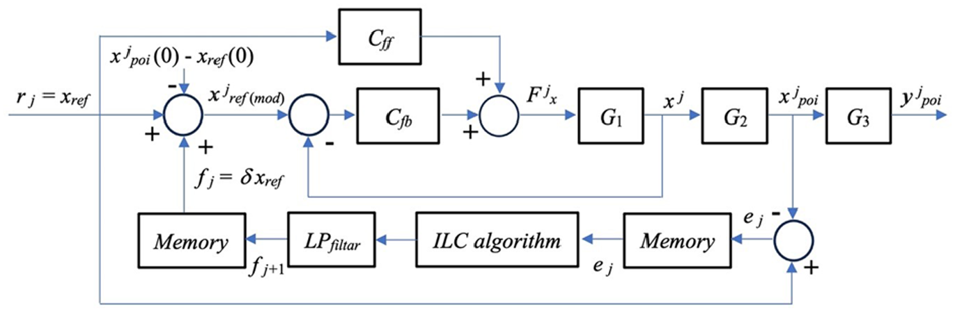
Structure of the closed-loop walking beam motion system with flexible coupled robotic mechanism with integrated feedforward controller and modified serial ILC connection.
The feasibility of filtering major input signals (setpoint, process output, and measurable load disturbances) to the PID controller is analyzed, yielding validated modifications for maintaining good system performance. 36 For instance, a low-pass filter can reduce overshoots during step changes in the setpoint:

The first-order filter eliminates step changes in the proportional component of the controller, while the second-order filter addresses changes in the derivative component during setpoint transitions. 36 In this context, Figure 6 proposes a structural modification (with the final proposed modification presented in Figure 12).
Since C ff (s) = Ms2, the second derivative of the reference trajectory significantly influences the dynamics of the control signal. A reference signal with rapid changes may cause the control signal to exceed actuator limits. While reference trajectories are generally designed to avoid unacceptable dynamics in control and output signals, the ILC algorithm aims to precisely track challenging reference trajectories, which may involve rapid dynamic changes. Consequently, the ILC signal can exhibit sharp variations and discontinuities. Similar to the approach in Hägglund, 36 the ILC signal could be filtered in a serial connection to mitigate undesirable dynamics in the control signal. However, proper implementation of the filter is challenging, as it risks adversely affecting previously achieved system performance.
Norm optimal ILC design: Modifications, simulation verification, results, and discussion
In the previous section, the signals and functionalities of the system components, as well as the overall setup illustrated in Figures 4 to 6, were discussed. This section focuses on the synthesis of the ILC algorithm, which aims to ensure the convergence of the compensation signal
The plant is modeled using discrete-time transfer functions
The plant model, including
The complementary sensitivity function of the system without the ILC algorithm (

The reference trajectory

An ILC algorithm can be expressed by its update equation:
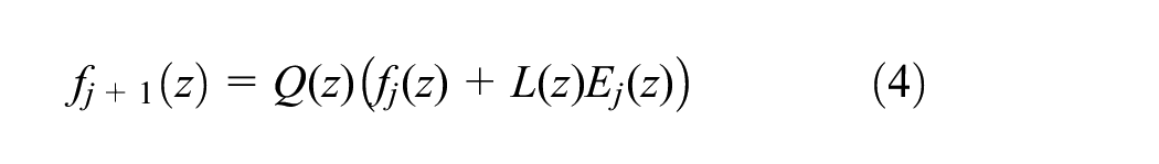
Here,
If relation (4) holds, the tracking error propagation for the system in Figure 5 is expressed as:

The first term determines how much of the previous error is propagated to the next iteration. The tracking error converges monotonically if and only if:

for all frequencies

However, this inversion is typically not exact due to system non-idealities or non-minimum phase behavior. In such cases, exact inversion is replaced by stable approximations, such as Zero Phase Error Tracking Control (ZPETC) or regularized inversion, which retain only the stable portion of the inverse. These non-causal approximations are implemented offline to preserve robustness while avoiding unstable dynamics.
Therefore,
For the controlled plant in Figure 1 and the ILC structure with serial connection, calculating

The impact of ILC signals
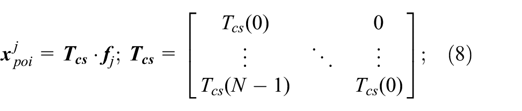
To derive the optimal update law for the ILC compensation signal

This relation assumes that the closed-loop system from
We now define a quadratic cost function that penalizes the tracking error

Substituting the expression for

Expanding this term:

The goal of the norm-optimal ILC design is to determine the compensation control signal

Differentiating the cost function with respect to

Rearranging the terms gives the linear system:

Solving the update equation yields the ILC update law:

Here, the learning and robustness matrices are defined as:


These expressions clearly demonstrate how the learning behavior is influenced by both system dynamics and the design of the weighting matrices. To ensure numerical stability and robustness of the ILC update law (12), we note that the matrix to be inverted in equations (13) and (14),

is symmetric and positive definite, provided that
The matrices
Generalization is achieved by appropriately selecting the weighting matrices to capture the expected variations in system dynamics and disturbances. As a result, the fixed matrices
To analyze the convergence of the update law (12) and the tracking error signal in the closed-loop control structure shown in Figure 5, we first express the tracking error as:

Substituting this into the update law (12) yields:

This expression reveals that the evolution of the ILC signal across iterations is governed by the iteration matrix:

Thus, a sufficient condition for the asymptotic convergence of the ILC signal to a steady-state solution is that the spectral norm of

where
Moreover, by substituting the ILC update equation (12) into the tracking error dynamics equation (9), we obtain:

This equation shows that the tracking error dynamics depend not only on the current error but also on the asymptotic behavior of the ILC signal

Notably, the inhomogeneous term

indicates that tuning
The convergence analysis highlights that the proposed norm-optimal ILC framework offers a structured approach for shaping the learning dynamics via the design of weighting matrices
The matrix
(1) A larger
(2) The matrix
Through proper tuning, the designer can balance convergence speed, robustness, and steady-state performance. The norm condition in equation (15) offers a practical criterion for verifying convergence and guiding the selection of weighting matrices.
Tuning of the weighting matrices 38 :
(1)
(2)
(3)
In the control system defined by Figures 1 and 5 (or 6), with controllers C ff and C fb designed as described in Section “System description,” and with the reference trajectory (7) defined over a finite time horizon of N samples, and parameters listed in Table 1, the following weighting matrices were used in the norm-optimal ILC cost function (10):

where
In Figure 6, we adopt a third-order Butterworth digital low-pass filter
Simulation results for the structure in Figure 6 and the norm-optimal ILC design procedure are shown in Figures 9 and 10. The presence of the

Illustration of the iterative convergence of the norm-optimal ILC algorithm and its impact on reducing the tracking error of the x-coordinate of the point of interest.

Illustration of the operation of the designed norm-optimal ILC structure from Figure 6.
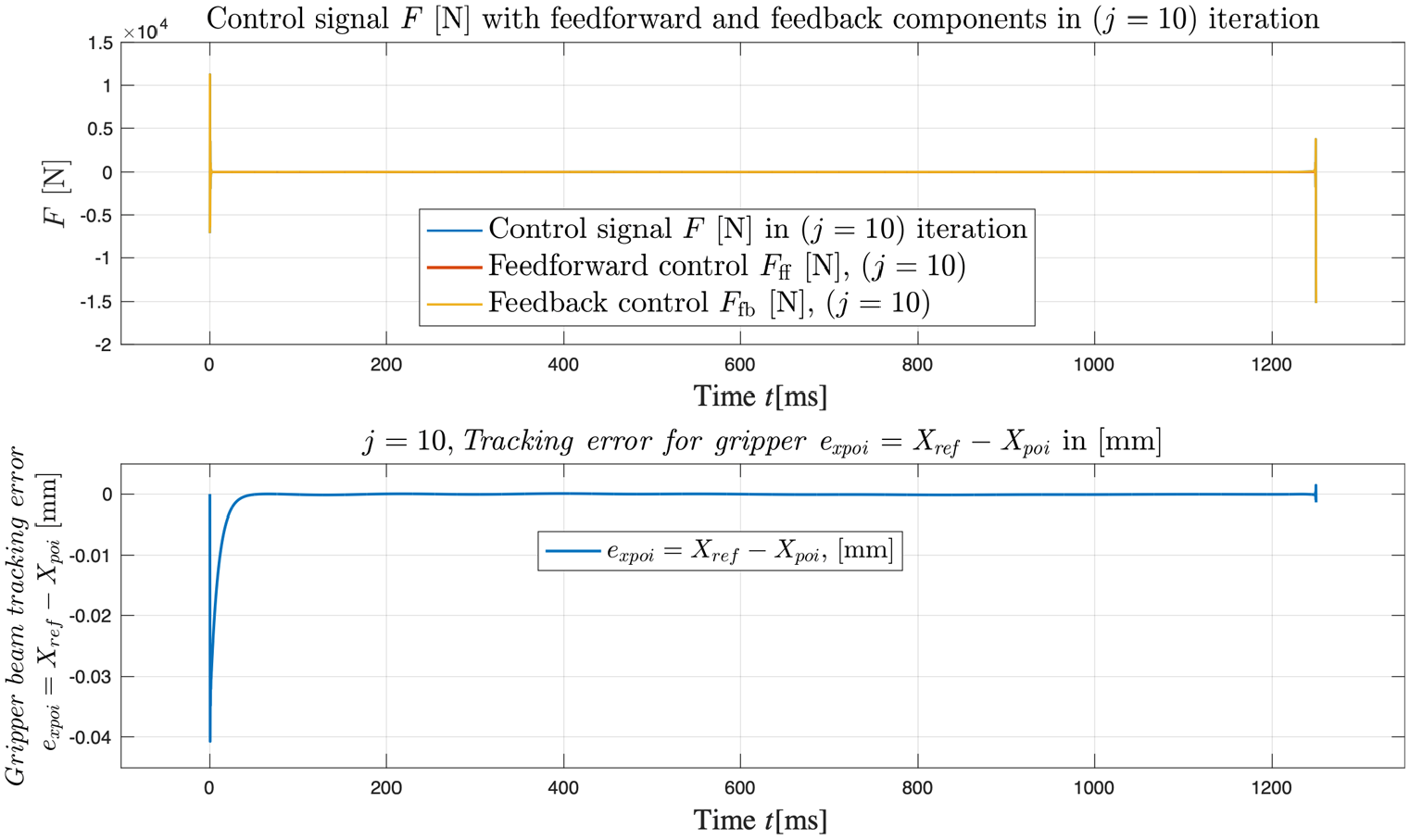
Illustration of the operation of the designed norm-optimal ILC structure from Figure 5.
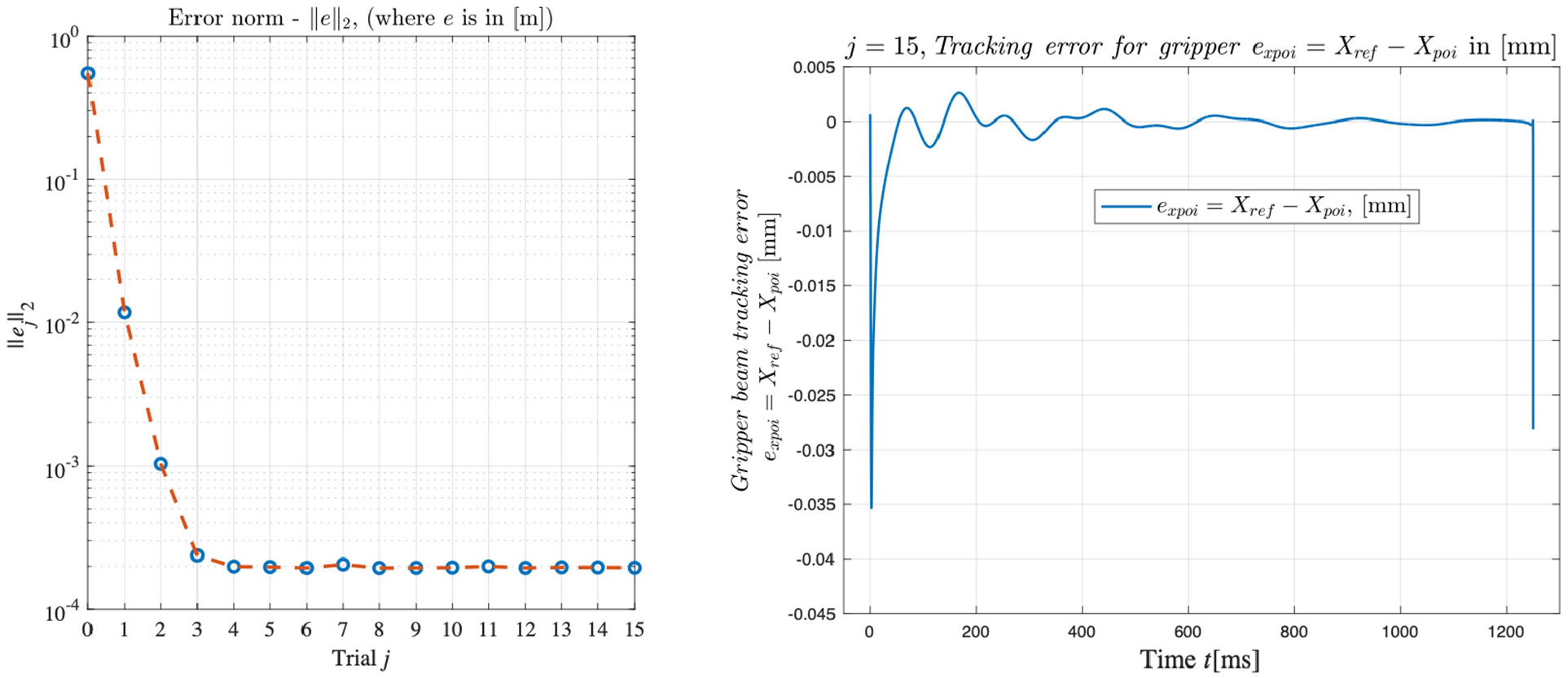
Illustration of the iterative convergence of modified norm-optimal ILC algorithm and its impact on reducing the tracking error of the x-coordinate of the point of interest.

Control signal of the modified norm-optimal ILC structure from Figure 6. (A non-causal low-pass filter (17) is used, and the last sample of the ILC signal is set to be equal to the penultimate one.).
The tracking error is reduced by over 1000 times with the application of the norm-optimal ILC algorithm. This algorithm enables more efficient tracking of the point of interest along the x-coordinate (
Simulation results indicate that while the norm-optimal ILC algorithm significantly improves the performance of the output variable, it is impractical due to its tendencies toward controller fragility, abrupt jumps, oscillations, and potentially excessive control variable values.
Modified norm optimal ILC
The ILC signal f j is calculated offline between consecutive iterations, aiming to achieve the most efficient tracking of the reference trajectory xref. In offline mode, non-causal filtering of the ILC signal f j is feasible, allowing noise suppression and reduction of abrupt changes in the control signal. However, such filtering can negatively impact the previously achieved performance of the output signal. Despite the small sampling time (T s = 2e-04 s), even a delay or lead in the filtered ILC signal as small as one sampling interval can significantly affect output signal performance.
To address controller fragility, we propose a heuristic solution validated through simulations. Specifically, we recommend incorporating a digital non-causal FIR filter:
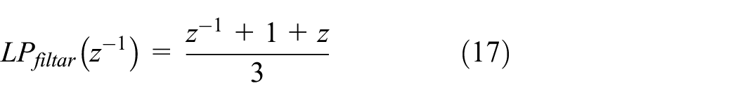
into the structure shown in Figure 6. This filter supplements the third-order Butterworth digital low-pass filter, previously applied with a bandwidth of 0.999·(1/

Structure of the closed-loop walking beam motion system with flexible coupled robotic mechanism and modified serial ILC connection and feedback controller implementation.

The FIR filter defined by (17) is a symmetric 3-point moving average filter, with frequency response:
where
The modification in Figure 12 introduces the feedback controller implementation as follows:

The integral action (
Based on the results in Figure 13, we conclude that the filter in equation (17) is unnecessary in the structure presented in Figure 12.
Excessive control actions observed at the end of the reference trajectory (Figure 9) are attributed to numerical instability. Extending the reference trajectory by a suitable time interval, Δt (e.g. 50 ms), enables the offline computation of the ILC signal f j to continue beyond the actual system implementation. This approach prevents abrupt jumps in the control signal at the trajectory endpoint.
At the beginning of the reference trajectory, sudden variations in the ILC signal—often caused by disturbances such as initial conditions—can also lead to excessive control actions and actuator saturation. The modified structure in Figure 12 effectively mitigates these discontinuities in the control variable.
This improvement becomes evident when comparing the control signal amplitudes across different configurations: approximately 10,000 N in Figure 9, 2000 N in Figure 11, and only 300 N in Figure 14. Considering realistic actuator limitations, the control signal in Figure 14 remains well within the acceptable range, in contrast to the excessive peaks observed in Figures 9 and 11.

Illustration of the operation of the designed norm-optimal ILC structure from Figure 12.
The effectiveness of the proposed modification becomes particularly evident under stringent actuator saturation limits. Figure 15 explicitly illustrates the iterative convergence of the tracking error norm under different actuator saturation thresholds, confirming that the modified ILC structure maintains system performance even when the actuator saturation level is as low as 30 or 20 N.
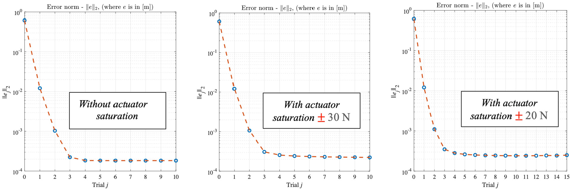
Illustration of the iterative convergence process for the tracking error norm in the structural implementation of the system from Figure 12, under different control signal constraints.
The fragility observed in our study does not stem from internal closed-loop instability, but rather from signal-level degradation in the control signal. These degradations are triggered by abrupt changes in the feedback controller input, caused by reference trajectory endpoints, discontinuities in the ILC signal, or mismatches in initial conditions. This phenomenon is particularly relevant for real-world implementations, where actuator saturation and excessive oscillations must be avoided.
In this paper, we characterize controller fragility as the sensitivity of control signal quality to small, abrupt perturbations in initial conditions, the reference trajectory, the ILC signal and other internal signal discontinuities, measurement noise, and minor variations in the controller’s structure and parameters. Specifically, we define controller fragility in terms of undesirable increases in control signal amplitude, sudden jumps, or high-frequency oscillations, triggered by minor structural or signal-level changes.
To quantify this phenomenon, we define the Control Signal Fragility Index (CSFI) as:

where
CSFI value greater than 0.5 indicates significant controller fragility—that is, a high sensitivity of the control signal to small, abrupt internal signal variations. The simulation results presented in Figures 8, 9, 11, and 14 suggest that unmodified controller structures exhibit high CSFI values, confirming their vulnerability. In contrast, the proposed modifications (e.g. the structure shown in Figure 12) result in markedly reduced fragility, consistent with lower CSFI values and improved robustness.
This paper introduces a general methodology aimed at reducing the sensitivity of the control variable to abrupt variations in the ILC signal when the signal is applied in series within a closed-loop control architecture. In this way, in serial ILC implementations within a closed-loop control structure, abrupt variations in the ILC signal can negatively affect both horizontal and vertical motion components. The proposed method relies on a structural decomposition of the feedback controller, whereby the integral component is retained in the direct path, and the remaining dynamics are relocated to the feedback path. This modification effectively mitigates, and in some cases eliminates, control signal degradation caused by discontinuities in the ILC signal.
Such discontinuities often arise because of attempts to compensate for disturbances associated with initial conditions. Consequently, when feasible, it is preferable to eliminate these disturbances through constructive (i.e. system-level or initialization) measures rather than through compensatory control action.
Conclusion
The walking beam motion system with a flexibly coupled robotic mechanism is widely used in industrial applications such as assembly lines, high-precision machines, and transport systems. Operating in repetitive cycles, it tracks a reference trajectory with high precision. However, increasing machine speeds to boost productivity poses challenges, as demanding reference trajectories can lead to more aggressive control signal changes and increased tracking errors. To maintain high-precision tracking of the desired trajectory, an exogenous or feedforward ILC signal can be integrated into the system.
This paper demonstrates that while the ILC signal can enhance precision, its integration into an existing feedback control system may introduce discontinuities and fluctuations in the control signal, potentially degrading overall performance. To address these challenges, the paper proposes structural modifications to the feedback control algorithm and the implementation of the ILC signal, ensuring improved system robustness and precision.
The paper begins with a literature review, highlighting that ILC implementations are highly specific to applications and that the associated implementation challenges represent an area for future research. It then presents a detailed procedure for synthesizing and implementing the norm-optimal ILC signal in the walking beam motion system. The findings show that, even when stability is positively confirmed, inadequate implementation of the feedback controller or improper integration of the ILC signal can result in unacceptable system performance and controller fragility.
Through simulation, the paper proposes and validates a robust implementation strategy for the feedback controller and ILC signal integration. All nonlinear effects in the walking beam motion system are accounted for in the simulation, and the norm-optimal approach to ILC signal synthesis is data-driven rather than model-based.
The proposed approach successfully mitigates controller fragility induced by the ILC signal, ensures feasible control variable dynamics, and achieves the desired system performance.
Although nonlinear friction was not explicitly modeled in the simulation environment, in practical implementation scenarios, friction compensation should be considered. If friction effects are consistent across repetitions, the ILC algorithm is expected to implicitly compensate for them. Otherwise, specialized control strategies for friction compensation may be used in combination with ILC.
Future work will focus on experimental validation of the proposed ILC methodology. A wirebonding machine is considered as a testbed for experimental validation of the proposed ILC methodology under real-world constraints.
Footnotes
Handling Editor: Divyam Semwal
Funding
The authors received no financial support for the research, authorship, and/or publication of this article.
Declaration of conflicting interests
The authors declared no potential conflicts of interest with respect to the research, authorship, and/or publication of this article.