Research on tool tip wear detection and life prediction based on an improved L1PS model

Abstract

Tool wear is a critical factor that directly impacts product performance, making accurate and timely detection essential for ensuring machining quality. In particular, under conditions of shallow cutting depth, tool tip wear significantly exceeds edge wear, yet the detection of tool tip wear has received little attention. Therefore, this paper proposes an image segmentation algorithm for detecting milling cutter tip wear, enabling precise measurement of tool tip wear. Initially, Valley-emphasis method is employed for initial segmentation of ground images to detect and segment the bottom edges. Subsequently, the detected edges serve as masks for parallel computation, achieving precise edge segmentation. Finally, the XOR result of the finely segmented edges and the mask is used to determine the wear region. Compared to existing detection algorithms, this method enhances edge detection accuracy without increasing detection time. The maximum error compared to manual measurement is within 0.007 mm, with a minimum accuracy rate of 97.92%. Additionally, the algorithm’s runtime has been reduced to 15.53 s, a decrease of approximately 94.68%. These results substantiate the efficacy of the proposed approach.

Introduction

With the continuous development of China’s aerospace industry, there is an increasing demand for materials that are difficult to machine, complex structural components, and thin-walled parts, which have higher performance requirements. These components are typically processed using milling operations. In particular, thin-walled parts made of aircraft aluminum alloys are machined using high-speed, low-feed, and low-depth-of-cut techniques, enabling the complete processing of all relevant dimensions in a single clamping operation and requiring more precise dimensional and positional tolerances. During the milling process, friction between the milling cutter and the workpiece generates a significant amount of heat, resulting in the conversion of mechanical energy into plastic deformation. As the duration of friction increases, the tool experiences prolonged pressure, leading to tool wear. The performance of the milling cutter deteriorates with increasing tool wear and significantly affects surface integrity, machining efficiency, and surface properties during the machining process, often leading to process failure. According to surveys, the costs associated with tooling and tool changes account for 3%–12% of the total machining cost, and tool inspection contributes to downtime, accounting for 7%–20% of the total machining time. ¹ Abnormal tool conditions cause 10%–40% of machine downtime, ² with less than 38% of industrial tools reaching their expected service life. ³ Therefore, online detection of milling tool wear, also known as tool condition monitoring (TCM), is currently one of the research hotspots in academia and industry.

Currently, most methods for detecting milling tool wear in industrial production rely on empirical observation and offline measurements. Manual inspection is not only costly but also subjective, lacking the ability to quantify the degree of wear. In offline measurements, the tool and tool holder need to be repeatedly clamped and positioned, significantly reducing efficiency and introducing additional assembly errors and changes to the wear mechanism, which outweigh the benefits. Both methods require machine downtime for inspection, further decreasing machining efficiency and increasing enterprise costs.^4,5

In the recent scholarly landscape, there has been an upsurge of suggested solutions targeting wear detection, which can be broadly bifurcated into indirect and direct methodologies. The indirect approach employs apt sensors to harvest signals such as cutting forces, ⁶ acceleration and vibrations,^7,8 and temperature, ⁹ forging an association between these singular or conglomerate signals with the condition of tool wear.^10,11 Li and Zhu ¹² advocated for an empirical statistical model that estimates the in situ area of tool wear, incorporating both process parameters and force characteristics. Zhou et al. ¹³ introduced a TCM method that synergizes the optimal feature parameters of acoustic sensor signals with a dual-layer kernel extreme learning machine. Twardowski et al. ¹⁴ established a link between the vibration acceleration signal, serving as the model input data, and the wear value of the end-milling tool VBc. He et al. ⁹ proposed a stacked sparseautoencoder model to predict tool wear, utilizing raw temperature signals and backpropagation neural network regression. Stavropoulos et al. ¹⁵ simultaneously monitored acceleration and spindle drive current sensor signals, accomplishing tool wear prediction through a cubic regression model and a pattern recognition system. Lei et al. ¹⁶ proposed physically based models, statistically based models, data-driven models, and hybrid models. The indirect approach may be beneficial in practical applications; however, signal analysis fails to provide direct and accurate measurements of tool wear values, as signals are subject to influence from industrial environmental factors.^17,18

The direct approach is commonly referred to as a machine vision system, primarily implemented through charge-coupled device (CCD) cameras or optical microscopes. Direct tool condition monitoring focuses on the surface wear profile of the tool, the integrity of the workpiece surface, the morphology of the chips, and finer classification based on these outcomes. Fernández-Robles et al. ¹⁹ used various image processing techniques to assess the area of flank wear using micro-milling tool images. Li et al. ²⁰ established a probabilistic function based on the correlation principle between the grayscale variations along the cutting edge and the relative positions of the original and worn boundaries, reconstructing the curved original tool boundary through Bayesian inference. Lim et al. ²¹ utilized a deep learning regression model to predict tool wear states from features extracted from 2D images of the workpiece surface profile. Pagani et al. ²² extracted different indicators from the RGB and HSV image channels to guide a neural network in chip classification, indirectly assessing tool wear. Zhang et al. ²³ proposed a theoretical approach to monitor ultra-precision rake face milling tool wear by observing changes in chip morphology. García-Ordás et al. ²⁴ classified the wear of form milling tools using machine learning and computer vision techniques. The direct method has the advantage of non-contact and accurate values, but has three major problems: difficult image acquisition, inability to detect online, and complex algorithms.

In this paper, the real-time online detection of milling cutter bottom tip wear area is achieved through machine vision algorithms. The milling cutter bottom images are collected in real time by designing CNC programs and controlling tool installation. Environmental light interference is reduced by adjusting the combination of light sources. An improved image processing algorithm is employed to detect the wear area of the tool tip, ensuring measurement accuracy while reducing computational time and addressing the issue of limited tool sample quantity. This provides a novel approach to online detection using machine vision.

Related works

Image segmentation is a fundamental task in many image processing and computer vision applications.^25–27 Its objective is to transform an image into a collection of pixel regions with specified labels, enabling the localization, differentiation, and measurement of labeled objects. In practical applications of tool wear detection, accurate segmentation becomes challenging due to issues such as complex tool structures, uneven illumination within the machine tool, and excessive edge fluctuations during the acquisition process, leading to significant measurement errors and unreliable results.

Currently, image segmentation algorithms can be classified into two main categories: deep learning algorithms and foundational algorithms. Deep learning has proven to be a powerful tool in signal detection and image processing, allowing for pixel classification based on training data. However, deep learning typically involves millions of trainable parameters, and successful training heavily relies on large, accurately labeled datasets. Additionally, deep learning lacks a solid mathematical foundation and often suffers from unexpected side effects, such as adversarial attacks. ²⁸ In contrast, foundational algorithms, such as various thresholding methods and variational energy functional methods, exhibit strong stability and adaptability. Thresholding methods generally segment images based on pixel grayscale values, including Otsu, K-means, and KSW entropy algorithms. These methods are simple, computationally efficient, and can be flexibly customized to meet different requirements. Variational energy functional methods and their numerical solution strategies are easy to control and implement, suitable for various tasks. ²⁹ Among them, active contour models (ACMs) have been proposed by numerous researchers, and effective numerical computation formulas have been provided.

The Otsu method and its improvements

The Otsu method is a commonly used generic image thresholding method. By selecting the threshold with the largest inter-class variance or the smallest intra-class variance from the image histogram, the Otsu method can obtain satisfactory segmentation results when the target and the image background have similar variances. However, the method fails if the target and the image background differ significantly in size. In other words, the Otsu method works well for bimodal histograms but fails for images with a single-peaked distribution or near-single-peaked histogram.

The image can be described as $F(x,y)$ with a gray scale ranging from 0 to $L-1$ , where $L$ is the number of different gray levels. The probability of occurrence of a gray level $k$ is defined as follows:

$$p\left(k\right)=\frac{1}{\mathrm{MN}}\sum _{F(x,y)=k}f(x,y).$$

(1)

If the image is divided into two classes, $D_0$ and $D_1$ , using a threshold $t$ , then $D_0$ consists of pixels with gray values in $[0,t]$ and $D_1$ consists of pixels with gray values in $[t+1,L-1]$ . Let ${\omega }_0\left(t\right)$ and ${\omega }_1\left(t\right)$ denote the cumulative probability of class $D_0$ and $D_1$ , respectively. The probabilities satisfy:

$$\begin{array}{c}{\omega }_0=\sum _{0<k\le t}p\left(k\right),\hfill \\ {\omega }_1=\sum _{t<k\le L-1}p\left(k\right),\hfill \\ {\omega }_0+{\omega }_1=1.\hfill \end{array}$$

(2)

Let ${\mu }_0\left(t\right)$ and ${\mu }_1\left(t\right)$ denote the average levels of classes $D_0$ and $D_1$ , respectively, and the mean grayscale values of these two classes can be calculated as:

$$\begin{array}{cc}\multicolumn{1}{c}{{\mu }_0\left(t\right)}& =\frac{\sum _{0<k\le t}\mathrm{kp}\left(k\right)}{{\omega }_0\left(t\right)},\hfill \\ \multicolumn{1}{c}{{\mu }_1\left(t\right)}& =\frac{\sum _{t<k\le L-1}\mathrm{kp}\left(k\right)}{{\omega }_1\left(t\right)},\hfill \end{array}$$

(3)

and ${\mu }_T$ be the global mean of the image:

$${\mu }_T={\omega }_0{\mu }_0+{\omega }_1{\mu }_1.$$

(4)

Then for a threshold $t$ , the inter-class variance of $D_0,D_1$ is expressed as:

$$E={\omega }_0{({\mu }_0-{\mu }_T)}^2+{\omega }_1{({\mu }_1-{\mu }_T)}^2.$$

(5)

The optimal threshold $g$ can be determined as:

$$g=\arg \underset{0<t\le L-1}{\max }[{\omega }_0{({\mu }_0-{\mu }_T)}^2+{\omega }_1{({\mu }_1-{\mu }_T)}^2].$$

(6)

The image is then binarized according to the optimal threshold $g$ :

$$h(x,y)=\{\begin{array}{cc}1,\hfill & g\le F(x,y)<L-1,\hfill \\ \multicolumn{1}{c}{0,}& 0\le F(x,y)<g.\hfill \end{array}$$

(7)

The idea of the Valley-emphasis (VE) method is to attach a weight to Otsu’s objective function and express equation (5) as follows:

$$E^{\prime }=(1-h\left(t\right))[{\omega }_0{({\mu }_0-{\mu }_T)}^2+{\omega }_1{({\mu }_1-{\mu }_T)}^2],$$

(8)

where $h\left(t\right)=p\left(t\right)$ . This ensures that when the selected threshold has a high probability of occurring (a large $p\left(t\right)$ ), a very small weight is assigned so that $E^{\prime }$ cannot be maximized, and conversely a larger weight is obtained. ³⁰ This valley search method chooses a threshold that maximizes the variance between classes and lies at the bottom of the valley between the two peaks of the gray-scale histogram.

Active contour models (ACMs)

Based on the characteristics of active contours, ACMs can be categorized into edge-based models^31,32 and region-based models.^33,34 Edge-based models primarily rely on edge gradient information and are suitable for segmenting images with high contrast and well-defined edges, but they often fail on noisy images. Region-based models are less sensitive to initialization and perform better with noise and weak edges by using information like region mean median, variance, and texture distributions.

In region-based models, the Chan-Vese (CV) model ³⁴ simplifies the Mumford-Shah (MS) model by assuming each segmented subregion is homogeneous, allowing for the segmentation of piecewise constant images. The model employs the level set method (LSM) ³⁵ to represent regions and boundaries, exhibiting favorable mathematical properties. Building upon this, Jung ³⁶ proposed a piecewise smooth model to address intensity inhomogeneity and employed an $L_1$ data fidelity measure to handle outliers and noise effectively. This model effectively addresses image non-uniformity using image decomposition theory and demonstrates robustness against noise and outliers.

MS model

Let $\mathrm{\Omega }\subseteq {\mathbb{R}}^2$ be a bounded image domain with the Lipschitz boundary and $I\left(x\right):\mathrm{\Omega }\to \mathbb{R}$ be a given image. The image domain $\mathrm{\Omega }$ is assumed to be partitioned into two regions ${\mathrm{\Omega }}_1$ and ${\mathrm{\Omega }}_2$ such that ${\mathrm{\Omega }}_1\cap {\mathrm{\Omega }}_2=Ø$ and ${\mathrm{\Omega }}_1\cup {\mathrm{\Omega }}_2=\mathrm{\Omega }$ . Note that ${\mathrm{\Omega }}_1$ refers to the region of interest in this paper. Furthermore, we set the constants $c_1$ and $c_2$ to denote the average intensities of two regions ${\mathrm{\Omega }}_1$ and ${\mathrm{\Omega }}_2$ . The MS model considered to approximate an image by using piecewise smooth functions as:

$$\underset{s\left(x\right),\Gamma }{\min }\{\lambda {\int }_{\mathrm{\Omega }}{|I\left(x\right)-s\left(x\right)|}^2\mathrm{dx}+\beta {\int }_{\mathrm{\Omega }\setminus \Gamma }{|\nabla s\left(x\right)|}^2\mathrm{dx}+\mathrm{Length}\left(\Gamma \right)\}.$$

(9)

where $\lambda$ and $\beta$ are the positive parameters and $|\nabla s\left(x\right)|=\sqrt{{\left({\partial }_{x_1}s\left(x\right)\right)}^2+{\left({\partial }_{x_2}s\left(x\right)\right)}^2}$ . The first term is the data fitting term. $s\left(x\right)$ is a smooth approximation of the given image $I\left(x\right)$ except on the edge set $\mathrm{\Gamma }$ . The last term represents the edge length of the edge curve $\mathrm{\Gamma }$ .

L1PS model

By assuming that the true image is the sum of a piecewise-constant function and a smooth function, a piecewise-smooth image segmentation model with $L_1$ data fidelity (L1PS) is considered as follows:

$$\{\begin{array}{c}\begin{array}{cc}\underset{c_1,c_2,B\left(x\right),u\left(x\right)\in C_1}{\min }\hfill & \lambda {\int }_{\mathrm{\Omega }}\left(\begin{array}{c}|I\left(x\right)-c_1-B\left(x\right)|u\left(x\right)+\hfill \\ \multicolumn{1}{c}{|I\left(x\right)-c_2-B\left(x\right)|(1-u\left(x\right))}\end{array}\right)\mathrm{dx}\hfill \\ \multicolumn{1}{c}{}& +\beta {\int }_{\mathrm{\Omega }}{|\nabla B\left(x\right)|}^2\mathrm{dx}+\nu {\int }_{\mathrm{\Omega }}|\nabla u\left(x\right)|\mathrm{dx}\hfill \\ \multicolumn{1}{c}{\mathrm{s}.\mathrm{t}.}& u\left(x\right)=\{\begin{array}{cc}1,\hfill & \mathrm{if}x\in {\mathrm{\Omega }}_1,\hfill \\ \multicolumn{1}{c}{0,}& \mathrm{if}x\in {\mathrm{\Omega }}_2.\hfill \end{array}\hfill \end{array}\hfill \end{array}$$

(10)

where $c_1,c_2$ are constant intensities for the foreground and background, $B\left(x\right)$ is a smooth background function, $u\left(x\right)$ is the indicator function, and $C_1=[0,1]$ is a convex relaxation of $u\left(x\right)$ . ²⁷ Using a convex relaxation scheme, the model becomes:

$$\begin{array}{cc}\underset{c_1,c_2,B\left(x\right),u\left(x\right)\in C_1}{\min }\hfill & \lambda {\int }_{\mathrm{\Omega }}\left(\begin{array}{c}|I\left(x\right)-c_1-B\left(x\right)|u\left(x\right)+\hfill \\ \multicolumn{1}{c}{|I\left(x\right)-c_2-B\left(x\right)|(1-u\left(x\right))}\end{array}\right)\mathrm{dx}\hfill \\ \multicolumn{1}{c}{}& +\beta {\int }_{\mathrm{\Omega }}{|\nabla B\left(x\right)|}^2\mathrm{dx}+\nu {\int }_{\mathrm{\Omega }}|\nabla u\left(x\right)|\mathrm{dx}\hfill \end{array}$$

(11)

In equation (11), the $L_1$ data-fitting term enables segmentation of images with low contrast or outliers, the second term enforces smoothness of $B\left(x\right)$ everywhere, and the last term is the total variation which denotes the length of the boundary. ³¹

Methodology

The tool wear online detection system is composed of an image acquisition module and an image processing module, as shown in Figure 1. The image acquisition module divides the workbench into two parts: the detection area and the processing area, and utilizes the detection area to set up the image acquisition equipment for image capture. The image processing module is based on a self-matching algorithm. The image processing is performed in two steps: segmenting the multi-edge image into single-edge images and segmenting the worn region of each individually segmented edge. The flowchart of the image processing module is shown in Figure 2.

Figure 1.

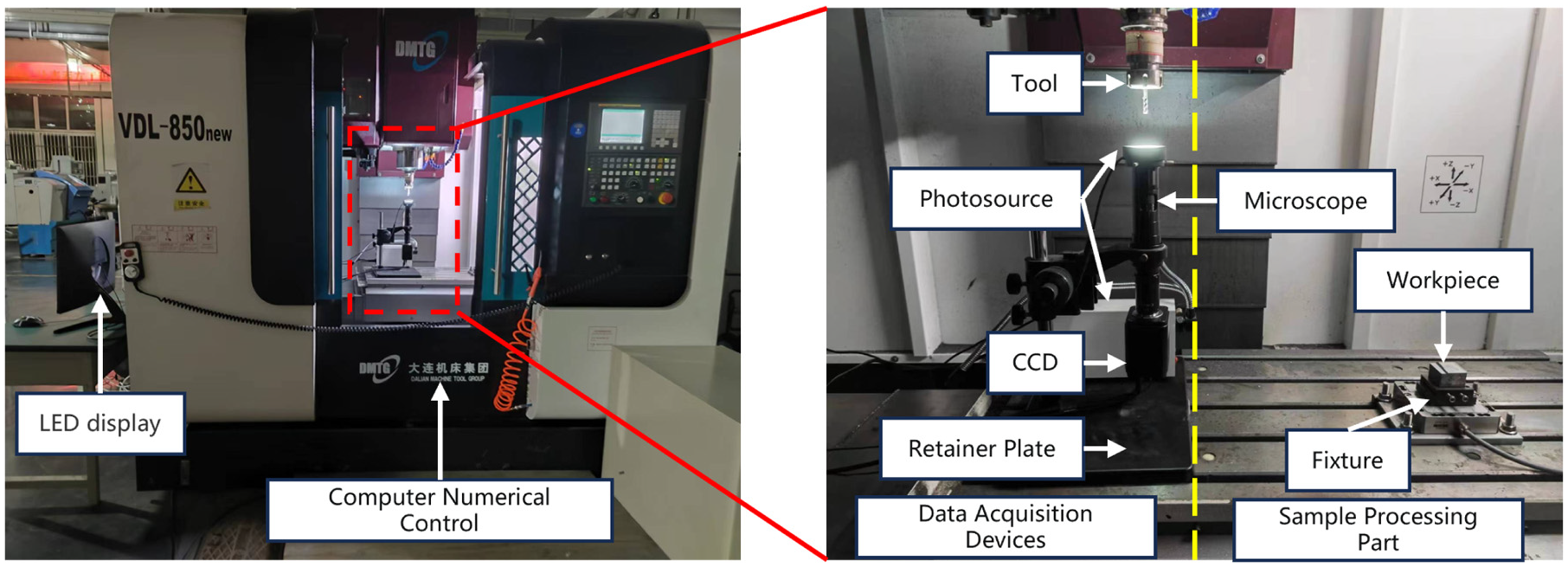
Experimental setup used for obtaining tool wear images.

Figure 2.

Overall flowchart of image processing module.

Image acquisition

This paper presents an online detection approach that divides the image acquisition module into an acquisition system and a control system. The acquisition system consists of a camera, a microscope, an adjustable LED ring light, and an adjustable linear cold light source, enabling the capture of cutting edge images in a single pass. The intensity of the light source is pre-set based on the ambient light and the pre-experimental image capture results, as illustrated in Figure 3. The control system utilizes numerical control machine tools and programming codes to implement spindle speed reset and tool position movement. The programming code follows the rule of setting a fixed processing time in the code, during which the tool disengages from the work surface, moves to a fixed coordinate above the camera, the spindle stops rotating (n = 0), the feed speed becomes 0 (F = 0), and a pause of 5 s is specified. After the image capture is completed, the spindle starts rotating again, and the tool returns to its original position to continue executing the remaining program.

Figure 3.

Results of online image acquisition: (a) Roberts and (b) acquisition effect with fixed extension length.

Image processing

L1PS can flexibly handle irregular boundaries and shapes in images, providing excellent segmentation performance for blurry edges, particularly suitable for edge wear regions with highly blurred boundaries and smooth transitions in base edge images. However, L1PS has some limitations. The method is not suitable for multi-object segmentation and is sensitive to the initial region. Additionally, it has high computational complexity, requiring excessive computation time when applied to the entire base edge image. Therefore, this paper proposes an improved method, where the image is first segmented using the VE algorithm. The segmentation results not only transform the image into single-object tasks but also provide initial masks for L1PS. The detailed steps are as follows:

Initial image segmentation

This study adopts the Valley-Emphasis (VE) algorithm for initial segmentation, where the threshold $T$ is determined according to equation (12).

$$T=\arg \underset{0\le t\le L-1}{\max }{E}^{\prime }\left(t\right)$$

(12)

To ensure consistency of symbols throughout the text, the segmentation results of (7) have been renamed as shown in equation (13).

$$G(x,y)=\{\begin{array}{cc}1,\hfill & T\le F(x,y)<L-1\hfill \\ \multicolumn{1}{c}{0,}& 0\le F(x,y)<T\hfill \end{array}$$

(13)

Milling cutter number identification

To accurately identify the number of cutting edges on a worn milling cutter, an improved method is proposed that combines morphological operations and Hough Transform. This method involves applying threshold segmentation, followed by morphological processing, Hough Transform line detection, and finally analyzing the angle distribution to determine the number of cutting edges.

Morphological operations

Morphological opening and closing operations are performed on the binary image using the same structuring element to remove noise and enhance the features of the cutting edges.

Hough Transform for line detection

The Hough Transform is used to detect lines in the edge-detected image. This technique works by transforming points in the Cartesian coordinate system into the parameter space, where lines are represented by their distance and angle from the origin, facilitating the identification and analysis of straight line features.

Filtering and merging lines

To filter out short lines and merge closely spaced lines with similar angles, the following criteria are used:

First, the length $L$ of each detected line is calculated, where $(x_1,y_1)$ and $(x_2,y_2)$ are the two endpoints of the detected line, $l$ represents a detected line, and $A$ represents the set of all detected lines.

$$L=\sqrt{{(x_2-x_1)}^2+{(y_2-y_1)}^2}$$

(14)

Second, only lines longer than a specified minimum length $L_{\min }$ are kept. Where $L_c$ indicates a line that meets the length requirements.

$$L_c=\{l\in A\mid L>L_{\min }\}$$

(15)

Third, lines that are close to each other and have similar angles within a threshold ${\theta }_t$ are merged. Where, $\alpha$ is the Angle of the line, and M- $L_c$ is the merged line. $\alpha =\arctan 2(y_2-y_1,x_2-x_1)\times \frac{180}{\pi }$

$$\mathrm{M}-L_c=\mathrm{merge}(L_c,{\theta }_t)$$

(17)

Analyzing angle distribution

The angle distribution of the lines is analyzed, and the number of significant peaks in the histogram is identified, corresponding to the number of cutting edges on the milling cutter (N).

Single-edge image extraction

After identifying the number of cutting edges on the milling cutter, the complete image of the cutter is segmented into parts, each containing a single cutting edge. The segmentation results are shown in Figure 4.

Figure 4.

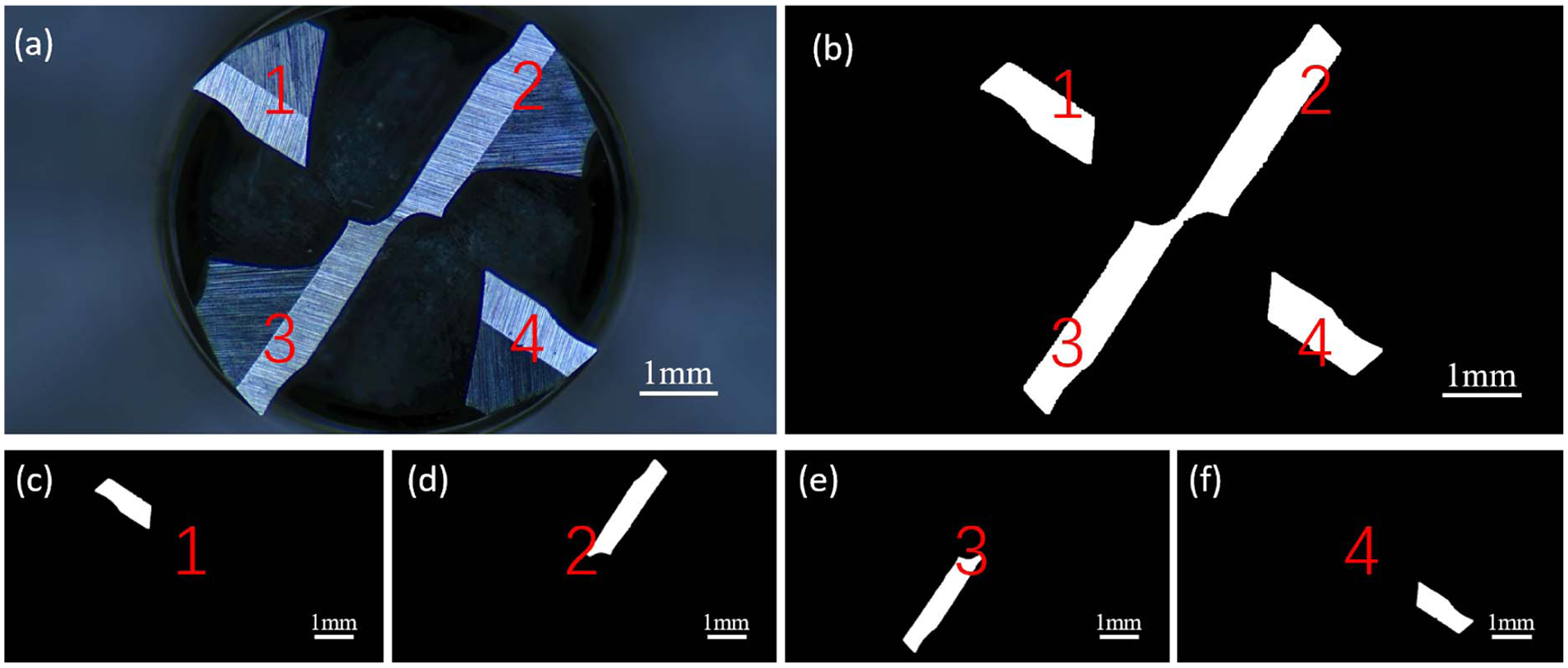
The result of single-objective image extraction: (a) grayscale image, (b) segmented cutting edge result, and (c–f) sub-images of the cutting edges corresponding to the numbers in the image.

Calculate segment boundaries

For a cutter with $N$ cutting edges, each segment covers an angular range of:

$$\mathrm{\Delta }\theta =\frac{{360}^{°}}{N}$$

(18)

Create masks for each segment

For each segment, a binary mask is created. The mask covers the angular range from ${\theta }_i$ to ${\theta }_i+\mathrm{\Delta }\theta$ :

$$M_i(x,y)=\{\begin{array}{cc}1,\hfill & \mathrm{if}{\mathrm{\theta }}_{\mathrm{i}}\le \mathrm{\theta }(\mathrm{x},\mathrm{y})<{\mathrm{\theta }}_{\mathrm{i}}+\mathrm{\Delta }\mathrm{\theta },\hfill \\ \multicolumn{1}{c}{0,}& \mathrm{otherwise},\hfill \end{array}$$

(19)

where $\theta (x,y)$ is the angle of the point $(x,y)$ with respect to the center of the image.

Apply masks to the image

The image is segmented by applying each mask to the original image $F(x,y)$ :

$$F^{\prime }(x,y)=F(x,y)·M_i(x,y),$$

(20)

where $F^{\prime }(x,y)$ is the segmented image corresponding to the $i$ -th cutting edge.

The edge image of a single cutting edge is given by:

$$P(x,y)=\mathrm{edge}(G(x,y)·M_i(x,y)),$$

(21)

where $G(x,y)$ is the gray image and $M_i(x,y)$ is the segmentation mask.

Detailed image segmentation

Using edge images as masks

As shown in Figure 5, global thresholding methods may fail to provide accurate segmentation in complex structures, especially when the tool is worn. The L1PS algorithm, which accounts for intensity inhomogeneity, provides superior edge segmentation results. The edge image $P(x,y)$ obtained from the previous steps is used as a mask for detailed segmentation of the initial base edge image $F^{\prime }(x,y)$ using L1PS. This process is performed in parallel based on the number of cutting edges. The level set method is employed to handle irregular boundaries and shapes in the image, yielding accurate edge segmentation $S(x,y)$ .

Figure 5.

The segmentation results of the proposed algorithm: (a) original image, (b) the single-objective mask, (c) VE segmentation result, and (d) final segmentation results.

L1PS algorithm rewrite

The L1PS algorithm uses the L1 norm (Manhattan norm) to effectively handle outliers and noise in image decomposition, addressing intensity inhomogeneity and demonstrating robustness to noise and outliers. It ensures smooth transitions between worn and unworn cutting edges.

Given the edge image $P(x,y)$ as a mask, the detailed edge extraction for the single-target original image $F^{\prime }(x,y)$ results in the wear edge image $S(x,y)$ . The process is defined as follows:

Let $\mathrm{\Omega }\subset {\mathbb{R}}^2$ be the bounded image domain. The single-target original image $F^{\prime }(x,y)$ is decomposed as:

$$F^{\prime }(x,y)=B(x,y)+J_i(x,y)+n(x,y),$$

(22)

where $B(x,y)$ represents the bias field image, $J_i(x,y)$ (for $i=1,2$ ) represents the true image for the foreground and background regions respectively, and $n(x,y)$ represents the noise image.

The L1PS model minimizes the following objective function to obtain the wear edge image $S(x,y)$ :

$$\{\begin{array}{cc}\underset{j_1,j_2,B(x,y),P(x,y)}{\min }\hfill & \lambda {\int }_{\mathrm{\Omega }}[|F^{\prime }(x,y)-j_1-B(x,y)|P(x,y)\hfill \\ \multicolumn{1}{c}{}& +|F^{\prime }(x,y)-j_2-B(x,y)|(1-P(x,y))]\mathrm{dx}\hfill \\ \multicolumn{1}{c}{}& +\beta {\int }_{\mathrm{\Omega }}{|\nabla B(x,y)|}^2\mathrm{dx}+\nu {\int }_{\mathrm{\Omega }}|\nabla P(x,y)|\mathrm{dx}\hfill \\ \multicolumn{1}{c}{\mathrm{s}.\mathrm{t}.}& P(x,y)=\{\begin{array}{cc}1,\hfill & \mathrm{if}\mathrm{x}\in {\mathrm{\Omega }}_1,\hfill \\ \multicolumn{1}{c}{0,}& \mathrm{if}\mathrm{x}\in {\mathrm{\Omega }}_2.\hfill \end{array}\hfill \end{array}$$

(23)

where $j_1$ and $j_2$ are the mean intensity values of regions ${\mathrm{\Omega }}_1$ and ${\mathrm{\Omega }}_2$ respectively, and $\lambda$ , $\beta$ , $\nu$ are positive parameters. The term $\beta {\int }_{\mathrm{\Omega }}{|\nabla B(x,y)|}^2\mathrm{dx}$ measures the intensity inhomogeneity using the ${\mathcal{L}}_2$ norm, while the term $\nu {\int }_{\mathrm{\Omega }}|\nabla P(x,y)|\mathrm{dx}$ measures the length of the edge image $P(x,y)$ using the ${\mathcal{L}}_1$ norm to preserve edge smoothness. The optimized $P(x,y)$ is taken as the wear edge image $S(x,y)$ .

Optimization process

To solve the above model, one main difficulty of the numerical implementation is the binary constraint. To this end, we define a convex set $C_1:=[0,1]$ and then use the convex relaxation scheme to transform the optimization problem accordingly:

$$\begin{array}{cc}S(x,y)=\underset{j_1,j_2,B,P\in C_1}{\min }\hfill & \lambda {\int }_{\mathrm{\Omega }}(|F^{\prime }(x,y)-j_1-B|P+\hfill \\ \multicolumn{1}{c}{}& |F^{\prime }(x,y)-j_2-B|(1-P))\mathrm{dx}\hfill \\ \multicolumn{1}{c}{}& +\beta {\int }_{\mathrm{\Omega }}{|\nabla B|}^2\mathrm{dx}+\nu {\int }_{\mathrm{\Omega }}|\nabla P|\mathrm{dx}\hfill \end{array}$$

(24)

The minimization problem is not convex with respect to $(j_1,j_2,B(x,y),P(x,y))$ but is convex with respect to each variable individually. Each sub-minimization problem has a precise solution, which can be computed using convex optimization algorithms. The problem is solved by alternating minimization: fixing $P(x,y)$ to compute the minimum of $j_1,j_2,$ and $B(x,y)$ , and then using these to compute the minimum of $P(x,y)$ . While this process does not guarantee convergence to the global minimum (or even a local minimum), in practice it often yields a good approximation. Therefore, the numerical solution $(j_1,j_2,B(x,y),P(x,y))$ is determined using the alternating minimization method.

Calculating the wear area

The number of pixels within the wear region of the milling cutter tip is determined by comparing the wear edge image $S(x,y)$ with the edge image $P(x,y)$ , as in equation (25). The wear area $B$ is then calculated based on the number of pixels in this region. An image processing algorithm is employed to calculate the number of pixels that fall within the wear region. These regions are characterized by differences between the $S(x,y)$ and $P(x,y)$ images. Each pixel in the wear region represents a small portion of the tool surface that has been worn away. The total wear area $B$ is calculated by summing the pixels within these regions:

$$B=\sum _{x,y}(S(x,y)\oplus P(x,y)),$$

(25)

where $B$ represents the total wear area, and $\oplus$ denotes the XOR operation.

In the initial step, camera calibration was performed to determine the actual size represented by each pixel, enabling the conversion of pixel count to actual physical dimensions. This calibration allows for precise measurement of wear based on the area. The discrepancies between the $S(x,y)$ and $P(x,y)$ images are identified and quantified by counting the pixels in the highlighted regions. The calibrated data is then used to convert this pixel count into an accurate physical measurement of the wear area.

Experimentation and discussion

Test equipment

In this study, a three-axis machining center was employed for tool wear testing, achieving a milling accuracy of 1 µm. The milling path followed a parallel reciprocating motion along the $Y$ -axis, utilizing uncoated high-speed steel tools, while the workpiece material selected was 45 steel, as shown in Figure 6.

Figure 6.

Tool path.

The quality of the collected images is a key factor in ensuring the effectiveness of the algorithm. Therefore, during the equipment setup process, special attention was given to controlling the lighting conditions and the machining environment.

Lighting conditions: Although the machine operates in a closed environment, external light interference cannot be completely eliminated. To mitigate this, we combined a ring light source with a linear light source. The ring light helps to supplement and reduce ambient light disturbances, while the linear light source enhances the contrast between the tool’s cutting edge and the background.

Processing environment: During normal machining, the tool is influenced by cutting fluids and chips, which can significantly affect image quality. In our study, we first employed a dry environment to avoid the effects of cutting fluids, and second, we continuously blew away debris to keep the tool surface clean.

In this research, the hardware environment is Intel^® Core™ i5-6600K @ 3.50GHz × 4 CPU, 8GB of memory, and the development environment is MATLAB 2018b. The image acquisition equipment is two strip light sources and an industrial camera with a resolution of 1200 × 1600.

To ensure data reliability and consistency of working conditions, each milling cutter mills a total of three layers of workpieces and is determined to be scrapped, while a new cutter and new workpieces are replaced. The specific machining parameters are detailed in Table 1.

Table 1.

Detailed machining parameters.

Parameters	Milling form	Cutting width	Cutting depth	Spindle speed	Feed rate
Value	Dry milling	0.1	1	800	600
Unit	N/A	mm	mm	m/min	mm/s

Algorithm analysis

Segmentation evaluation method

In order to quantitatively evaluate the segmentation results of various segmentation models, this study employs several evaluation metrics to assess the accuracy of image segmentation, including Jaccard similarity (JS), Misclassification Error (ME), Pixel Accuracy (PA), F1-Score (F1), and Kappa coefficient ( $\kappa$ ). ³⁷

Jaccard similarity (JS) measures the similarity between two sets of data by calculating the number of elements that are the same and different. The formula is defined as follows:

$$\mathrm{JS}=\frac{|S_1\cap {\mathrm{S}}_2|}{|S_1\cup {\mathrm{S}}_2|},$$

(26)

where $|·|$ denotes the area of the region, $S_1$ represents the segmentation result obtained using the algorithm, and $S_2$ represents the ground truth segmentation result.

Misclassification Error (ME) measures the percentage of background pixels misclassified as foreground and foreground pixels misclassified as background. For a binary segmentation problem, the ME can be simply expressed as:

$$\mathrm{ME}=1-\frac{|B_{\mathrm{gt}}\cap B_t|+|O_{\mathrm{gt}}\cap O_t|}{\left|B_{\mathrm{gt}}\right|+\left|O_{\mathrm{gt}}\right|},$$

(27)

where $B_{\mathrm{gt}}$ and $O_{\mathrm{gt}}$ represent the background and object in the ground truth image, and $B_t$ and $O_t$ represent the background and object in the thresholded segmentation image, respectively, where $|·|$ denotes the cardinality of a set. For a perfectly thresholded image, ME is 0, while for a completely misclassified thresholded image, ME is 1.

Another measure is to simply calculate the percentage of correctly classified pixels in the image. This measure is commonly referred to as Pixel Accuracy (PA) and is defined as:

$$\mathrm{PA}=\frac{\mathrm{TP}+\mathrm{TN}}{\mathrm{TP}+\mathrm{TN}+\mathrm{FP}+\mathrm{FN}},$$

(28)

where TP represents the number of correctly segmented foreground pixels, TN represents the number of correctly segmented background pixels, FP represents the number of incorrectly segmented foreground pixels, and FN represents the number of incorrectly segmented background pixels. In binary classification problems, PA is equal to $1-\mathrm{ME}$ .

F1-Score (F1) is a measure of classification accuracy in statistical analysis. It takes into account both precision and recall of the classification model. The F1-score can be seen as the harmonic mean of precision and recall. The formula is defined as follows:

$$F_1=\frac{2\mathrm{PR}}{P+R},P=\frac{\mathrm{TP}}{\mathrm{TP}+\mathrm{FP}},R=\frac{\mathrm{TP}}{\mathrm{TP}+\mathrm{FN}},$$

(29)

where $P$ represents precision and $R$ represents recall.

Kappa coefficient ( $\kappa$ ) is a statistical measure used to assess the agreement between two raters or judges who classify items into mutually exclusive categories. It is generally considered a more reliable measure than simple percentage agreement since $\kappa$ takes into account the possibility of agreement occurring by chance. The formula is defined as follows:

$$\begin{array}{c}\kappa =\frac{P_0-P_e}{1-P_e},\hfill \\ \multicolumn{1}{c}{P_e=\frac{(\mathrm{TP}+\mathrm{FN})(\mathrm{TP}+\mathrm{FP})+(\mathrm{FP}+\mathrm{TN})(\mathrm{FN}+\mathrm{TN})}{{(\mathrm{TP}+\mathrm{TN}+\mathrm{FP}+\mathrm{FN})}^2},}\end{array}$$

(30)

where $P_0$ is the sum of the number of samples correctly classified for each class divided by the total number of samples, which represents the overall classification accuracy, and $P_e$ is the probability of chance agreement.

Analysis of initial image segmentation algorithm

Upon observing the structure of the cutting tool, (1) noticeable wear marks are generated due to friction at the bottom of the blade, with significant and uneven distribution of these marks. Denoising algorithms fail to effectively address this issue, resulting in the formation of holes on the surface during the segmentation process. (2) The cutting tool consists of a handle and a blade, causing the blade’s helical line and the outline of the handle to not overlap, creating background regions for both the handle and the chip flute, with some grayscale differences between them.

Figure 7 and Table 2 show the segmentation results of different algorithms. Figure 7(a) shows the original collected image of the milling cutter, which is used for comparing the effects of various segmentation algorithms and does not participate in the evaluation of segmentation algorithms.

Figure 7.

Comparison of segmentation results of different methods: (a) original collected image, (b) OTSU algorithm, (c) VE algorithm, (d) Adaptive Local Thresholding, (e) Fast K-Means algorithm, and (f) Canny Edge Detection with Filling.

Table 2.

Evaluation metrics for different segmentation algorithms.

Method	JS	ME	PA	F1	Kappa
OTSU algorithm	0.000723	0.473344	0.526656	0.001432	−0.1575
VE algorithm	0.830850	0.014615	0.985385	0.917865	0.909879
Adaptive Local Thresholding	0.424708	0.114274	0.885726	0.583066	0.528377
Fast K-means algorithm	0.275841	0.227280	0.772720	0.422581	0.335283
Canny Edge Detection with Filling	0.460821	0.083306	0.916694	0.665942	0.624256

OTSU algorithm

The OTSU algorithm’s evaluation metrics all performed poorly, as shown in Figure 7(b). The Jaccard Similarity (JS) and F1-Score (F1) are almost zero, indicating that this algorithm almost failed to identify the correct regions in the segmentation task. The Misclassification Error (ME) is close to 50%, indicating a very high rate of misclassification. The Pixel Accuracy (PA) is slightly above 50%, showing the randomness of the algorithm. The Kappa coefficient is negative, indicating that the OTSU algorithm’s segmentation performance is even worse than random guessing, showing serious systematic errors. In summary, the OTSU algorithm performs extremely poorly in segmenting the milling cutter image and cannot effectively distinguish between the blade and the background.

VE algorithm

The VE algorithm performs best in all evaluation metrics, as shown in Figure 7(c). The Jaccard Similarity (JS) and F1-Score (F1) are both above 0.9, indicating that the algorithm can accurately identify most of the correct segmentation regions. The Misclassification Error (ME) is very low, and the Pixel Accuracy (PA) is close to 100%, demonstrating the high precision of this algorithm. The Kappa coefficient is close to 1, further verifying the high reliability and consistency of the VE algorithm. In summary, the VE algorithm excels in segmenting the milling cutter image and is the most recommended method.

Adaptive Local Thresholding

The performance of the Adaptive Local Thresholding algorithm is moderate, as shown in Figure 7(d). The Jaccard Similarity (JS) and F1-Score (F1) indicate that the algorithm can correctly identify segmentation regions to a certain extent, but there is room for improvement. The Misclassification Error (ME) and Pixel Accuracy (PA) show that the algorithm can correctly classify most pixels, but some misclassifications still exist. The Kappa coefficient shows that the algorithm has a certain level of consistency, but improvement is needed. In summary, the Adaptive Local Thresholding algorithm performs generally in segmenting the milling cutter image and requires further optimization.

Fast K-means algorithm

The performance of the Fast K-means algorithm is poor, as shown in Figure 7(e). The Jaccard Similarity (JS) and F1-Score (F1) indicate that the algorithm has limited ability to identify correct segmentation regions. The Misclassification Error (ME) is high, and the Pixel Accuracy (PA) shows that the algorithm correctly classifies most pixels but still has many misclassifications. The Kappa coefficient is low, indicating poor consistency of the algorithm. In summary, the Fast K-means algorithm performs poorly in segmenting the milling cutter image and needs improvement in segmentation accuracy.

Canny Edge Detection with Filling

The Canny Edge Detection with Filling algorithm performs well, as shown in Figure 7(f). The Jaccard Similarity (JS) and F1-Score (F1) indicate that the algorithm can identify many correct segmentation regions. The Misclassification Error (ME) is low, and the Pixel Accuracy (PA) is high, showing that the algorithm can correctly classify pixels in most cases. The Kappa coefficient is high, indicating good consistency between the segmentation results and the ground truth. In summary, the Canny Edge Detection with Filling algorithm performs well in segmenting the milling cutter image, but from a visual inspection, it introduces redundant information on each tooth, which is not conducive to further processing.

Overall, the VE algorithm performs best across all evaluation metrics, demonstrating high precision and consistency. The Canny Edge Detection with Filling and Adaptive Local Thresholding algorithms perform well but introduce too much redundant information, which is not beneficial for subsequent calculations. The OTSU and Fast K-means algorithms perform poorly, exhibiting significant systematic errors, and cannot be applied to the algorithms in this paper.

The primary reason for the poor performance of the comparison algorithms is that this study focuses on tool tip wear, while most previous research has concentrated on edge wear. In edge wear studies, the region of interest is typically larger, and by controlling data acquisition methods, the gray value difference between worn and unworn areas is more pronounced. In contrast, the region of interest in tool tip wear images occupies only a very small portion of the overall image, as shown in Figure 5, and has gray values similar to the background, making most algorithms ineffective for segmenting tool tip images.

Based on the structural analysis, the VE algorithm was chosen to segment the cutter teeth. However, the results of the VE algorithm still contain some redundant data. After segmentation using the VE algorithm, morphological opening operations are employed to disconnect the connections between wear marks, as shown in Figure 8(a). Subsequently, isolated points in the binary image are removed, and morphological closing is performed to fill in the holes, completing the segmentation of the cutter teeth, as shown in Figure 8(b).

Figure 8.

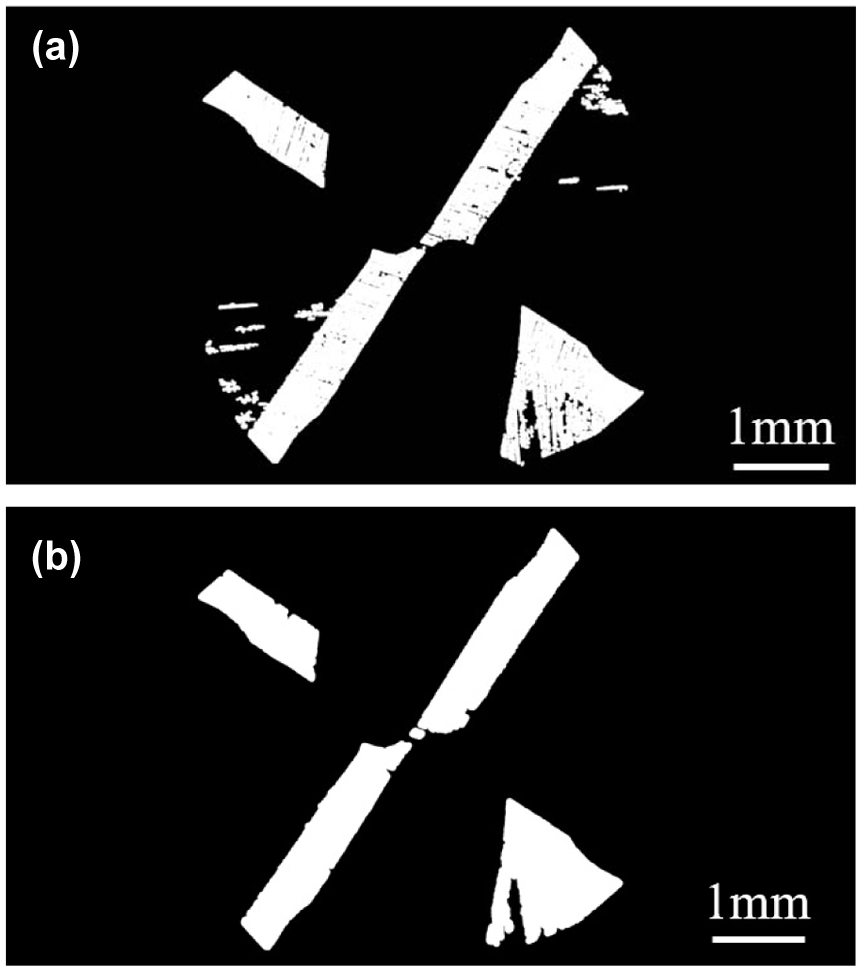
Morphological processing result: (a) morphological open operation and (b) removal of solitudes.

L1PS algorithm analysis

Figure 9 and Table 3 show the influence of different initial contours on the L1PS algorithm.

Figure 9.

The influence of different initial contours on L1PS algorithm.

Table 3.

Evaluation metrics for different initial contours in L1PS algorithm.

Initial contour	JS	ME	PA	F1	Kappa
Square – Left	0	0.467007	0.532993	NaN	−0.158574
Square – Center	0.609793	0.032583	0.967417	0.765677	0.748903
Square – Top	0.178185	0.078194	0.921806	0.276128	0.247424
Rectangle – Horizontal	0	0.465835	0.534165	NaN	−0.158474
Rectangle – Vertical	0	0.465835	0.534165	NaN	−0.158474

Square – Left

The segmentation result with this initial contour is extremely poor. The Jaccard Similarity (JS) is 0, indicating no overlap between the segmentation result and the ground truth. The Misclassification Error (ME) is close to 47%, and the Pixel Accuracy (PA) is only 53%, indicating that the algorithm’s performance is almost random. The F1-Score could not be calculated, and the Kappa coefficient is negative, showing that the segmentation result is even worse than random guessing, indicating significant systematic errors.

Square – Center

The segmentation result with this initial contour is the best, with excellent performance in all metrics. The Jaccard Similarity (JS) is 0.609793, indicating a high overlap between the segmentation result and the ground truth. The Misclassification Error (ME) is only 3.26%, and the Pixel Accuracy (PA) is as high as 96.74%. The F1-Score is 0.765677, and the Kappa coefficient is 0.748903, demonstrating high accuracy and consistency of the algorithm with this initial contour.

Square – Top

The segmentation result with this initial contour is moderate. The Jaccard Similarity (JS) is 0.178185, indicating a certain degree of overlap between the segmentation result and the ground truth. The Misclassification Error (ME) is 7.82%, and the Pixel Accuracy (PA) is 92.18%. The F1-Score is 0.276128, and the Kappa coefficient is 0.247424, indicating that the segmentation performance is acceptable but still has room for improvement.

Rectangle – Horizontal

The segmentation result with this initial contour is poor, similar to Square – Left. The Jaccard Similarity (JS) is 0, the Misclassification Error (ME) is 46.58%, and the Pixel Accuracy (PA) is 53.42%. The F1-Score could not be calculated, and the Kappa coefficient is negative, indicating that the segmentation performance is worse than random guessing and has systematic errors.

Rectangle – Vertical

The segmentation result with this initial contour is the same as Rectangle – Horizontal, also showing poor performance. The Jaccard Similarity (JS) is 0, the Misclassification Error (ME) is 46.58%, and the Pixel Accuracy (PA) is 53.42%. The F1-Score is undefined, and the Kappa coefficient is negative, indicating that the segmentation performance is poor and has significant systematic errors.

In summary, the segmentation results with Square – Left, Rectangle – Horizontal, and Rectangle – Vertical initial contours are poor, even worse than random guessing, indicating systematic errors. The segmentation result with the Square – Top initial contour is moderate. The best segmentation result is achieved with the Square – Center initial contour, demonstrating that the L1PS algorithm performs best under this initial contour. Nevertheless, it is evident that the L1PS algorithm alone is not suitable for multi-object segmentation, highlighting the effectiveness of the proposed algorithm in this paper.

It is evident that the L1PS model produces varying segmentation outcomes under different initial contours. Among them, the results obtained from (a), (d), and (e) exhibit similarities but fall short of achieving the desired segmentation. On the other hand, (b) and (c) reveal that although the L1PS model may not be suitable for multi-target segmentation tasks, it performs well in terms of single-object segmentation when appropriate initial contours are provided. Table 4 shows the running time and iteration counts of the L1PS and proposed methods. It can directly reflect the effectiveness of the method in this paper.

Table 4.

Iterations and CPU time of the L1PS and proposed method.

Segmentation result	Iterations	CPU time (s)
Square – Left	3401	292.22
Square – Center	1271	109.21
Square – Top	562	48.29
Rectangle – Horizontal	1475	126.73
Rectangle – Vertical	1624	139.54
Segmentation result	Iterations	CPU time (s)
Left-top	151	12.97
Right-top	105	9.02
Left-bottom	76	6.53
Right-bottom	131	11.26
Global	…	15.53

Verification of wear area

Figure 10 illustrates the wear curve of a milling cutter tip over time, showing the area of tip wear (in mm²²) against working time (in hours). The curve includes the actual wear data, the proposed method’s prediction, and the deviation. The red dashed lines indicate thresholds for different stages of wear, such as initial wear, slight wear, tip breakage, and tool damage. Additionally, the figure includes images of the tool tip wear at various stages.

• Initial wear (0–1.1 h): In the initial stage, when the tool travel is within the range of 2736 m, the wear area of the tool tip gradually increases, representing the normal wear period where the cutting edge adapts to the cutting conditions.

• Slight wear (1.1–3.6 h): When the tool travel is between 2736 and 7776 m, the wear area increases more significantly but remains within controlled limits, marking the transition from initial wear to steady-state wear.

• Breakage initiation (3.6–4.5 h): When the tool travel is between 7776 and 9720 m, the wear area increases significantly, indicating that wear has become more severe and the tool tip has begun to break down.

• Tool damage (4.5–5 h): After the tool travel exceeds 9720 m, the wear area reaches its peak, indicating severe wear and damage. This suggests that the tool is no longer effective and must be replaced.

Figure 10.

Milling cutter wear curve.

The proposed method’s prediction closely follows the actual wear trend with slight deviations, demonstrating high accuracy and reliability. The wear morphology changes from initial wear to slight wear, followed by tip breakage, and finally tool damage. The proposed method provides a reliable prediction of the wear trend with minimal deviation from the actual data, highlighting the importance of monitoring wear stages for timely maintenance and replacement of the milling cutter.

Conclusion

This paper designs a machine vision based online tool wear accurate measurement system. The whole process control from machine control, light source combination, equipment selection to algorithm design provides a new idea for online machine vision monitoring. Among them, control the machine tool to go to the path and code to achieve off-line acquisition of tool bottom edge; combination of ring light source and fiber optic light source to attenuate the influence of ambient light; adopting multi-edge to single-edge approach, using VE results as a mask, and using L1PS as an accurate measurement algorithm for fine segmentation. After experimental verification, the maximum deviation from the actual value is 0.036 mm, the average is 0.007 mm, and the detection accuracy is as low as 90.94%, with an average of 97.92%, which verifies the effectiveness of the method. Furthermore, the algorithm’s runtime has been optimized to 15.53 s, reflecting an approximate reduction of 94.68%.