Sage Journals: Discover world-class research

Abstract

Transformers are critical components in power transmission and distribution systems. However, their performance may deteriorate over time due to multiple factors. To detect such issues, diagnostic techniques like vibration analysis and infrared imaging are commonly used. Among these, infrared imaging stands out as a non-contact method requiring only an infrared camera. Nevertheless, interpreting thermal images can be difficult, as visual differences between faulty and healthy conditions are often subtle and indistinguishable to the human eye. This paper proposes a novel approach for detecting and classifying nine transformer conditions using infrared thermal images combined with Ant Colony Optimization (ACO) and the K-Nearest Neighbors (KNN) algorithm. Features are extracted from the R, G, and B channels separately, and four statistical indicators are computed to generate a comprehensive feature matrix. ACO is used to optimize the feature selection based on classification accuracy. The method addresses the challenge of achieving high diagnostic accuracy while meeting the constraints of online implementation. Experimental results show that the proposed method can accurately distinguish between one healthy state and eight types of short-circuit faults, outperforming conventional techniques.

Keywords

transformer diagnosis infrared images fault detection feature extraction selection optimization classification

Introduction

Transformers are essential components in power transmission and distribution networks. They are responsible for stepping up the voltage for efficient energy transmission and stepping it down for distribution to end-users.¹ Given their crucial role, it is vital to maintain their continuous and reliable operation.

However, various factors can lead to performance degradation or failure, such as poor maintenance, winding short circuits, network overvoltage, lightning strikes, and the natural aging of components like rubber seals.²

To ensure dependable transformer operation, a proactive and effective maintenance strategy is essential. Condition-based preventive maintenance enables the early detection of potential defects, allowing technicians to take timely corrective action and avoid costly failures or unplanned outages.³

Numerous diagnostic techniques have been developed to detect transformer faults. For instance, Behkam et al.⁴ employed frequency response traces in conjunction with artificial intelligence to identify and locate early-stage transformer defects. Thomas et al.⁵ used Convolutional Neural Networks (CNNs) to determine the type, phase, and location of faults from current data. Li et al.⁶ analyzed winding vibrations to evaluate structural integrity, while Wu et al.⁷ utilized time-frequency spectrograms derived from raw vibration signals as inputs to a classifier. Other innovative approaches include Ghoneim et al.,⁸ who proposed a Whale Optimization Algorithm guided by an Adaptive Dynamic Polar Rose method and applied it to dissolved gas analysis (DGA), and Kumar et al.,⁹ who developed a smart sensor system to monitor silica-gel breather color changes under varying humidity. Sahri and Yusof¹⁰ addressed missing data issues in DGA datasets by employing K-Nearest Neighbor imputation using both Euclidean and Cityblock metrics.

However, all of these techniques rely on contact-based sensors, which may introduce measurement distortions and affect the reliability of the classification outcomes.¹¹

To overcome the limitations of contact-based methods, non-contact approaches such as infrared (IR) image analysis have gained prominence. This technique detects temperature variations; as electrical faults typically generate localized heating in transformer components.¹² Infrared thermography is widely used in industrial diagnostics and even medical imaging. One major advantage is its ability to detect early-stage anomalies before serious failures occur, thereby enhancing maintenance planning and reliability.

Several studies have investigated infrared-based diagnostic methods for transformers. dos Santos et al.¹³ integrated temperature measurements from transformer oil with AI techniques, achieving an accuracy of 86% in fault detection. Balabantaraya et al.¹⁴ introduced a modified VGG-16 model for thermal image-based diagnosis. Mahami et al.¹⁵ combined infrared imaging with the GIST descriptor technique, although without feature selection. Fang et al.¹⁶ tackled class imbalance by integrating Neighborhood Component Analysis (NCA) with KNN and Bayesian optimization for hyperparameter tuning.

Despite their promising results, these hybrid methods often increase computational complexity, limiting their feasibility for real-time deployment.

In this study, we propose a simple yet effective method for transformer fault classification using only KNN and a small number of selected features, making it well-suited for online implementation. Our approach integrates feature extraction from infrared images with machine learning classification. We begin by analyzing the RGB channels separately to construct a large feature matrix. Since this extensive matrix may slow real-time processing, feature selection is applied to retain only the most relevant features.^17,18 Ant Colony Optimization (ACO) is used for feature selection, followed by classification with the KNN algorithm.

The originality of our work lies in three key aspects. First, we introduce a unique feature extraction method by decomposing infrared images into three separate matrices (R, G, and B), setting the other channels to zero each time. Second, we combine this extraction technique with an optimization algorithm designed to maximize classification accuracy. Third, we identify a classifier that achieves high accuracy, exhibits good stability, and operates with a minimal feature set.

To validate our method, we tested it on a publicly available dataset containing infrared images of a transformer in eight fault conditions and one healthy state. Our results demonstrate that the proposed technique converges quickly and achieves high performance using only three features. We further compared our approach with other classifiers, including Support Vector Machine (SVM) and Decision Tree (DT). While DT performed well, it required nine features to achieve similar accuracy.

To determine the most stable classifier, we conducted multiple simulations and analyzed the mean and standard deviation of their performance metrics. Our findings indicate that the KNN classifier offers higher accuracy and greater stability while requiring fewer features, making it the most suitable choice for real-time transformer fault diagnosis.

The remainder of this paper is organized as follows. Section “Experimental study and analysis” presents the experimental study. Section “Features extraction” describes the feature extraction method. Section “Features selection and classification” covers the feature selection process, including the use of Ant Colony Optimization (ACO) and the K-Nearest Neighbors (KNN) classifier, which serves as the fitness function for ACO. Section “Results and discussion” presents the results and discussion. Finally, Section “Conclusion” provides the conclusion.

Experimental study and analysis

Experiments were carried out for different conditions of electrical transformers whose specification are presented in Table 1. Nine different states are considered, a healthy state and eight different cases of short circuit faults in common core winding.

Table 1.

Thermal camera properties and electrical transformer specifications.

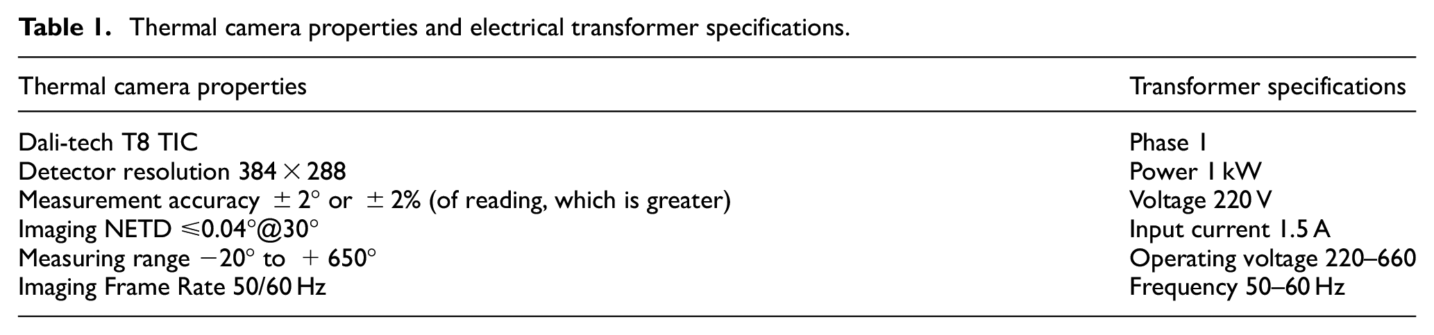
Thermal camera properties	Transformer specifications
Dali-tech T8 TIC Detector resolution 384 × 288 Measurement accuracy ±2° or ±2% (of reading, which is greater) Imaging NETD ≤0.04°@30° Measuring range −20° to +650° Imaging Frame Rate 50/60 Hz	Phase 1 Power 1 kW Voltage 220 V Input current 1.5 A Operating voltage 220–660 Frequency 50–60 Hz

Thermal images acquisition was performed on an Electrical Machines Laboratory workbench by a Dali-tech T4/T8 infrared thermal image camera at an environment temperature of 23°. Thermal camera properties and electrical transformer specifications are represented in Table 1. Nine sets (class label) of Images represent a healthy state and eight different faulty conditions of the transformer. As shown in Table 2 the first rang represents the number of short-circuit rounds from the set of 600 rounds, and the second rang represents the fault class percentage (%) of the number of short-circuit rounds.

Table 2.

The nine considered states in the transformer diagnostic.

Fault class (rounds)	Healthy	80	160	240	320	400	480	520	600
Fault class (%)	0	13	26	40	53	66	80	93	100
Class label	1	2	3	4	5	6	7	8	9

Figure 1 presents thermal images of both healthy and faulty transformer states. It is evident that visually distinguishing between these thermographs is extremely challenging. The minimal differences between the thermal images of healthy and faulty conditions make it nearly impossible to detect faults with the naked eye, increasing the risk of misclassification. This limitation highlights the need for advanced artificial intelligence (AI) and machine learning techniques to enhance fault differentiation and improve diagnostic accuracy.¹⁹

Figure 1.

Heat-thermal image of electrical transformer: (a) healthy, (b) 13% fault, (c) 26% fault, (d) 40% fault, (e) 53% fault, (f) 66% fault, (g) 80% fault, (h) 93% fault, and (i) 100% fault.

The studied faults are internal issues within the transformer, where short circuits occur in the windings located around the same magnetic core. This can lead to overheating, insulation failure, reduced performance, or even complete device breakdown. It is a serious type of internal fault often used for diagnostic testing or condition monitoring. The considered dataset includes eight short-circuit cases at different levels as shown in Table 2.

Features extraction

In this work, we separated the RGB images to three images R, G, and B images, for the R-image, we took the first matrix of RGB image and we forced the others to zeros, for G-image we took the second matrix and we forced the others to zero and with the same way we obtained the B-image as shown by the Figure 2.

Figure 2.

R-image, G-image, and B-image.

To construct the feature matrix, we extracted four statistical indicators: standard deviation, mean, maximum, and minimum values from each row of the image. The mathematical formulas for these indicators are provided in the following equations:

Mean

The mean can be defined as the mean color value in the image, which may define in equation (1)

μ = \frac{1}{N} \sum_{i = 1}^{N} x_{i}

(1)

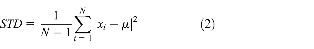
Standard deviation

The standard deviation is the square root of the distribution variation; equation (2) explain the of STD

STD = \frac{1}{N - 1} \sum_{i = 1}^{N} {| x_{i} - μ |}^{2}

(2)

Min

The min is the minimal color value in the image, the mathematical formula is shown in equation (3)

Min = \min | x_{i} |

(3)

Max

The max is the maximal color value in the image, the mathematical formula is shown in equation (4)

Max = \max | x_{i} |

(4)

The feature extraction method is illustrated in the following Figure 3:

Figure 3.

Features extraction method.

C1 is the first class (healthy state), the rest classes from C2 to C9 are the faulty classes, the obtained feature matrix is composed of 2760 features and 898 samples.

The first features represent the mean of the first row of the R image of each class, the second features represent the mean of the second row of the R image of each class and the last feature represent the mean of 230th row of the B image of each class.

Given this large number of features, it is recommended to make a selection to choose only the features who contains more information about the state of the transformer.

Features selection and classification

The extracted feature dataset often contains irrelevant or redundant features,²⁰ which can negatively impact classification performance. To achieve high accuracy in transformer fault classification, it is crucial to apply a feature selection process that eliminates unnecessary features while retaining only the most relevant ones.²¹ This not only enhances classification precision but also improves the overall efficiency of the fault diagnosis process.

In this study, we employ Ant Colony Optimization (ACO) for feature selection, using a fitness function based on the K-Nearest Neighbors (KNN) classification algorithm.

Ant colony algorithm (ACO)

The ant colony algorithm is a very popular method in the field of optimization and which is part of the field of swarm intelligence. The term “swarm” refers to a group of individuals who communicate with each other by interacting and modifying their environment.

Intelligence in this context means the intelligent behavior of an individual that is developed through the cooperation and interpretation of modifications made by each individual.

ACO was firstly introduced by Dorigo et al. in the early 1990s.²² It was considered a new nature-inspired metaheuristic method to solve optimization problems such as TSP problems.²³

When the ants look for food, each ant deposits a substance called pheromone, this substance is immediately detected by the other ants and follows the same path and in turn deposits new pheromones thus the old pheromones will be reinforced, consequently will be more marked by pheromones and will have a high probability of being followed by other ants.

Paths that are followed by fewer ants will see the pheromones deposited evaporate over time, so the most practiced path will be retained by the group by following the largest pheromone trail left by the group this concept is shown in Figure 4(a) and (b).

Figure 4.

Basic explanation of the ant colony algorithm.

The mathematical description of ACO

The updating of pheromones must be considered after each tour: this includes the quantity evaporated per unit length and deposited on the edge by the ant. The ants will choose and take the right path thanks to the mechanism of evaporation of pheromones. Thus, local optimization will be avoided. The intensity of pheromone on path-ij at time t + 1 is given by equation (5)²³:

τ_{ij} (t + 1) = ρ . τ (t) + Δ τ_{ij} (t, t + 1)

(5)

The value of the evaporation rate ρ is critical, When the evaporation rate is set to 1, there is no pheromone evaporation, and not easy to get convergence. But setting ρ too low is prone to get a local best answer.

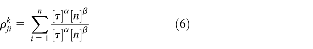
The transition probability for the k-th ant from nod i to nod j as equation (6)²³:

ρ_{ji}^{k} = \sum_{i = 1}^{n} \frac{{[τ]}^{α} {[n]}^{β}}{{[τ]}^{α} {[n]}^{β}}

(6)

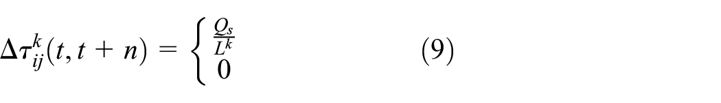
The trail update pattern determines the three categories that the field of the ant system (AS) can be divided to: ant-cycle, ant-quantity, and ant-density algorithms, their formulas are given by equations (7)–(9).²³ The ant-cycle model shows that each ant lays its trail at the end of the tour, but the other two model sup-dated the trail after each step, which explains the wide use of the Ant-cycle algorithm and the elimination of the two other models.

ANT-quantity:

Δ τ_{ij}^{k} (t, t + 1) = {\begin{matrix} \frac{Q_{s}}{L^{k}} \\ 0 \end{matrix}

(7)

ANT-density:

Δ τ_{ij}^{k} (t, t + 1) = {\begin{matrix} Q_{2} \\ 0 \end{matrix}

(8)

ANT-cycle:

Δ τ_{ij}^{k} (t, t + n) = {\begin{matrix} \frac{Q_{s}}{L^{k}} \\ 0 \end{matrix}

(9)

Where $Δ τ_{ij}^{k}$ is the quantity per unit of length of pheromone laid on edge (i, j) by the k-th ant between time t and t + 1; Q is a constant; d_ij is the Euclidean distance between i and j; L^k is the tour length of the kth ant.

Ant colony optimization for features selection

The application of the Ant Colony Optimization (ACO) algorithm to feature selection involves treating each feature as a node, representing a potential point along an ant’s path (see Figure 5). The number of features to be selected and the number of ants are predefined, and each ant constructs a subset of features accordingly. Once the selection phase is completed, an evaluation function is applied to the selected subsets, using the accuracy of a KNN classifier as the performance metric. Based on these results, pheromone levels are updated to reinforce the feature subsets that achieve the highest classification accuracy. This is done by using equation (9), where the distance L is replaced by one minus accuracy (1−acc).

Figure 5.

ACO problem representation for Features selection.

K-Nearest Neighbors (KNN)

The KNN algorithm is a classification and regression method, belongs to the class of supervised learning algorithm,²⁴ the advantage of this method is that it is very fast and easy to be implemented for online classification. The principle of the method is that if we have a new point to classify, we proceed to calculate the distance of this new point in relation to all the other points of the existing classes and the classification will be made according to the distance between this point with the classes.²⁴ The mathematical formula for the distances is given by equations (10) and (11).

Euclidian distance

d = \sqrt{\sum_{i = 1}^{n} {(x_{i} - y_{i})}^{2}}

(10)

Manhattan distance

d = \sum_{i = 1}^{n} {(x_{i} - y_{i})}^{2}

(11)

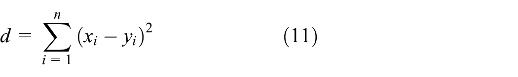
In this work we have used Euclidian distance.

In the example illustrated by the Figure 6, the distance calculated between the new point to the class C is smaller than the distance between the class A and B, so the new point is assigned to class C. The algorithm of the method is given by Figure 7.

Figure 6.

KNN classification.

Figure 7.

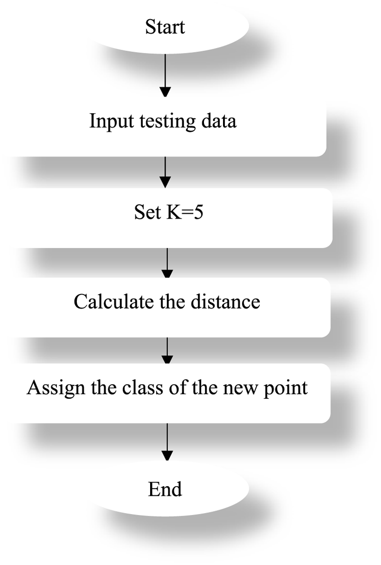
KNN algorithm.

The choice of K

To determine the optimal value of k, we conducted multiple simulations with and without feature selection, testing different values of k. For each simulation, we computed the standard deviation of accuracy to assess model stability. The results are presented in Table 3 (without optimization) and Table 4 (with optimization).

Table 3.

Best value of k without ACO (indicated in bold).

K	3	5	7	9	11
STD of ACC	1.68	1.52	2.17	1.79	1.53

Table 4.

Best value of k with ACO.

	K
Number of features	3	5	7	9	11
3	0.23	0	0.23	0.70	0.44
4	0.35	0.4	0.32	0	0.35
5	0	0	0.14	0	0.25
6	0	0	0	0.14	0.25
7	0	0	0	0	0
8	0	0.40	0	0.14	0.19
9	0	0	0	0	0
10	0.14	0	0.47	0.14	0.35

From Table 3, we observe that k = 5 yields the best result, as it has the lowest standard deviation. This indicates that the model is more stable with this value compared to other choices of k.

From Table 4, we see that the minimum number of features with the highest stability (STD = 0) is obtained for k = 5. Therefore, for the remainder of this study, we set k = 5 as the optimal value.

The principle of method is given by the following Figure 8:

Figure 8.

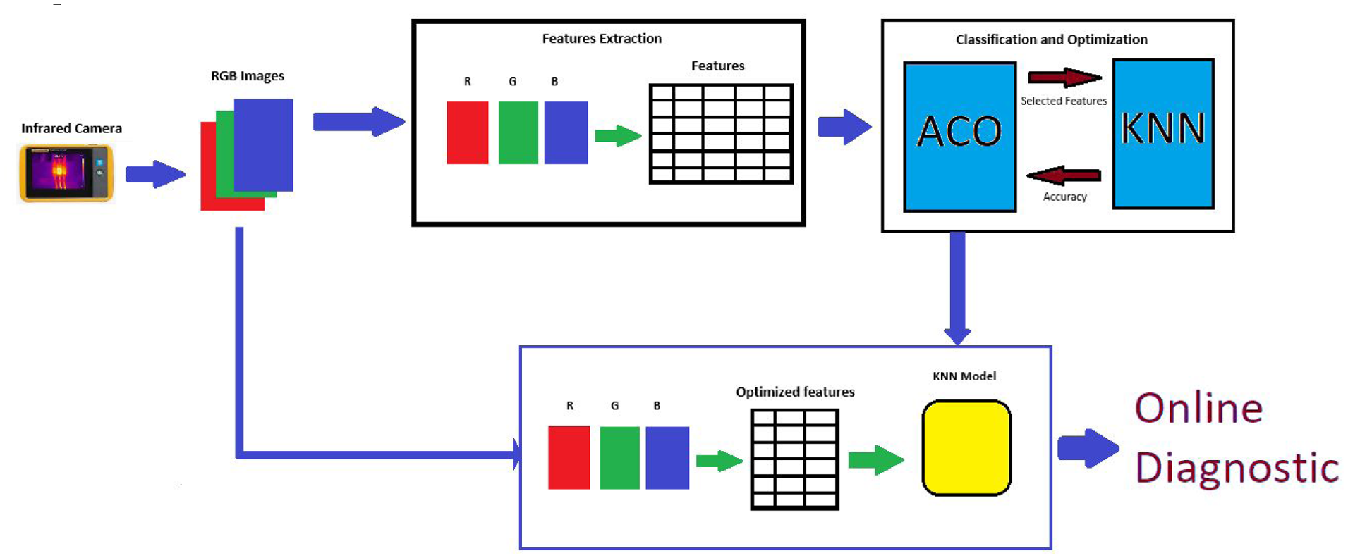
Flowchart of proposed method.

Figure 8 illustrates that the RGB images captured by the infrared camera are first separated into three individual channels. Then, a feature extraction phase is applied to each channel separately, resulting in a very large feature matrix. To address this, the ACO (Ant Colony Optimization) algorithm was introduced to optimize the number of features by using an objective function based on the accuracy of the KNN classifier. As a result, a significantly reduced feature set and a trained KNN model were obtained, which will be used for online diagnosis.

Results and discussion

This section presents the key findings of our study. The primary objective is to minimize the number of selected features while maintaining high classification accuracy.

To achieve this, the dataset was divided into two subsets: 80% for training and 20% for testing, using a confusion matrix to evaluate classification performance. Multiple simulations were conducted using the K-Nearest Neighbors (KNN) classifier with different feature subset sizes. The resulting classification accuracies are illustrated in Figure 9.

Figure 9.

Classification accuracy variation according to the features number.

As shown in Figure 9, when the number of selected features is between 3 and 10, the KNN classifier maintains high accuracy. However, beyond this range, the classification accuracy tends to decrease. These results confirm that KNN is highly effective even with a small set of features, which is particularly beneficial for real-time implementation due to reduced computational cost.

This observation is especially significant, as reducing the number of features substantially enhances computational efficiency, making the approach more suitable for practical, real-time diagnostic systems.

In Figure 9, three distinct zones can be identified: the first ranges from 3 to 10 features, the second from 11 to 15 features, and the third begins at 16 features onward. To do our study and cover all behaviors, we select a subset of 3 features from the first region, another of 11 features from the second region, and the last one of 20 features from the third region.

The following figure illustrates the classification results when using a small number of selected features, where the classifier processes 20 observations per class.

From Figure 10, we see that all diagonal elements in the confusion matrix are 100% indicates a perfect classification. In this context, each class was entirely and correctly identified by the model. This means there were no false positives or false negatives for any class. Additionally, the fact that all 20 observations were correctly classified reinforces the reliability of this result.

Figure 10.

Classification results with three features.

This level of performance, particularly when achieved with only three features, is notable. It suggests that these selected features are highly discriminative and sufficient to distinguish between classes effectively. The success of the model with a minimal feature set may indicate low noise and high signal relevance in those features.

In conclusion, 100% diagonal values and 20/20 correct classifications with three features indicate excellent model performance on this dataset. Nonetheless, further validation is recommended to confirm these findings and ensure the model’s generalization capabilities, for this the metrics: F1score, recall, specificity are used to prove the efficiency of the method.

The same result is obtained for four and five features.

In Figure 11(a), we observe that some observations are misclassified. Specifically, 95% of the observations are correctly classified, while 5% are misclassified, corresponding to 1 observation from 20 observations. As shown in Figure 11(b), this misclassified observation was predicted to belong to the 2nd class, but it actually belongs to the 1st class.

Figure 11.

Classification result with different features: (a, b) 11 features and (c, d) 20 features.

In Figure 11(c), we see that among all observations, only we five are misclassified. Here, 18 of the observations from 20 are correctly classified respectively in the first class and in the third class. In the fifth class, only one observation from 20 is misclassified.

The Figure 11(d) shows that among the misclassified observations, two observations were predicted to belong to the first class, whereas it belongs to the third class, while one observation was predicted to belong to the third class, but it belongs to the first class. Additionally, one observation was predicted to belong to the second class, while it belongs to the first class, and another was predicted to belong to the eighth class, but it actually belongs to the ninth class.

Even when considering other measurement metrics, the results are consistent and always shows that when the features number is small, the classification is excellent, as shown in the Table 5 below:

Table 5.

Results by considering other measurement metrics.

Metric	3 features					11 features					20 features
	Accuracy	Recall	F1score	Precision	Specificity	Accuracy	Recall	F1score	Precision	Specificity	Accuracy	Recall	F1score	Precision	Specificity
Result (%)	100	100	100	100	100	99.44	99.44	99.44	99.47	99.93	97.22	97.22	97.21	97.25	99.65

From the results, we conclude that the best performance is achieved when a small number of features is selected. Therefore, we focus only on the smaller set of features for the developed method and in the subsequent analysis.

To demonstrate the efficiency of the KNN classifier in the proposed method, we compared it with other classifiers, specifically the Decision Tree (DT) classifier and Support Vector Machine (SVM). We then conducted several simulations, where we calculated the classification accuracy based on the variation in the number of features. The results are presented in Figure 12.

Figure 12.

Classification accuracy variation as function of features number for KNN, DT, and SVM.

From the Figure 12, we see that the SVM starts with low accuracy (55%) when only one feature is used. Accuracy improves steadily as more features are added, reaching above 85% by 20 features. This indicates that SVM performances on this dataset are not good. However, the KNN achieves high accuracy early, close to 100% with just a few features. But, it shows some fluctuation as more features are added, with a slight drop at 20 features. The DT technique performs consistently well, achieving near-perfect accuracy, but this result is observed only when the number of features exceeds 10, and it remains stable across all higher feature number. This comparison indicates that KNN outperforms the other classifiers, as it achieves the highest accuracy with the fewest number of features, aligning with our goal of maximizing performance while minimizing feature number.

To determine which classifier remains stable when the number of features is very small (3, 4, 5), we need to analyze the stability of all classifiers.

Stability study

In this study, we conducted 20 experiments and computed the mean and standard deviation of all measurement metrics for each classifier. The results are presented in Table 6.

Table 6.

Comparison results of KNN, DT, and SVM.

	KNN			DT			SVM
Metrics	Features			Features			Features
	3	11	20	3	11	20	3	11	20
• Accuracy (%)	100	99.44	97.22	99.44	99.44	100	74.44	88.89	83.33
• STD (10⁻¹⁵)	0	0	0.45	0	0.56	0	0.22	0	0.22
• Recall (%)	100	99.44	97.22	99.44	99.44	100	74.44	88.89	83.33
• STD (10⁻¹⁵)	0	0.45	0.45	0.45	0.45	0	0.34	0.22	0.22
• Precision (%)	100	99.47	97.25	99.47	99.47	100	75.38	82.95	79.63
• STD (10⁻¹⁵)	0	0	0.45	0	0	0	0.22	0	0.22
• Specificity (%)	100	99.93	99.65	99.93	99.93	100	96.81	98.61	97.92
• STD (10⁻¹⁵)	0	0.22	0.45	0.22	0.22	0	0.22	0.22	0
• F1score (%)	100	99.44	97.21	99.44	99.44	100	70.60	85.04	79.26
• STD (10⁻¹⁵)	0	0	0.11	0	0	0	0.22	0.11	0.11

According to the first column of the table, we observe that all metrics yield good results, highlighting the effectiveness of KNN with ACO. A similar outcome is also observed with the Decision Tree (DT) classifier, as shown in column 6, but the number of features used is 20, which is higher than the three features utilized by KNN. Based on these results, we conclude that KNN provides excellent performance with a minimal number of features, making it well-suited for online implementation of our method.

Conclusion

In this study, we proposed a reliable and efficient method for diagnosing transformer faults using infrared thermal images. The approach integrates Ant Colony Optimization (ACO) for feature selection and K-Nearest Neighbors (KNN) for classification. The ACO algorithm identifies the most relevant features based on a fitness function driven by the classification accuracy of KNN. This combination ensures both high accuracy and model stability, while significantly reducing the dimensionality of the input data.

The method was evaluated on a dataset comprising one healthy condition and eight different short-circuit fault classes. Experimental results show that the proposed ACO-KNN technique achieves excellent performance with as few as three features, demonstrating its effectiveness for real-time implementation. Furthermore, comparative analysis with other classifiers, including Support Vector Machine (SVM) and Decision Tree (DT), confirmed that the ACO-KNN framework not only achieves superior accuracy but also requires fewer computational resources.

Overall, the proposed method offers a promising solution for intelligent transformer fault diagnosis using infrared imaging, combining simplicity, speed, and high diagnostic precision.

Footnotes

Handling Editor: Sharmili Pandian

ORCID iDs

Boualem Ikhlef

Chemseddine Rahmoune

Mohamed Amine Sahraoui

Funding

The author(s) received no financial support for the research, authorship, and/or publication of this article.

Declaration of conflicting interests

The author(s) declared no potential conflicts of interest with respect to the research, authorship, and/or publication of this article.

References

Wang

Liu

Chen

, et al. Power transformer fault diagnosis system based on Internet of Things. J Wireless Com Network 2021; 2021: 21.

Zhang

Song

Dual-aspect self-attention based on transformer for remaining useful life prediction. IEEE Trans Instrum Meas 2022; 71: 1–11.

Alsumaidaee

Yaw

Koh

, et al. Review of medium-voltage switchgear fault detection in a condition-based monitoring system by using deep learning. Energies 2022; 15(18): 6762.

Behkam

Karami

Naderi

, et al. Condition monitoring of distribution transformers using frequency response traces and artificial neural network to detect the extent of windings axial displacements. In: 2022 26th international electrical power distribution conference (EPDC), Tehran, Islamic Republic of Iran, 11–12 May 2022, pp.18–23. New York: IEEE.

Thomas

Chaudhari

Verma

NK.

CNN-based transformer model for fault detection in power system networks. IEEE Trans Instrum Meas 2023; 72: 1–10.

Chen

Yang

, et al. Convolutional neural network-based transformer fault diagnosis using vibration signals. Sensors 2023; 23(10): 4781.

Triebe

Sutherland

JW.

A transformer-based approach for novel fault detection and fault classification/diagnosis in manufacturing: a rotary system application. J Manuf Syst 2023; 67: 439–452.

Ghoneim

SSM

Farrag

Rashed

, et al. Adaptive dynamic meta-heuristics for feature selection and classification in diagnostic accuracy of transformer faults. IEEE Access 2021; 9: 78324–78340.

Kumar

Mishra

Islam

Condition monitoring of transformer breather using smart photodiodes array. IEEE Trans Instrum Meas 2024; 73: 1–7.

10.

Sahri

Yusof

RB.

Support vector machine-based fault diagnosis of power transformer using k nearest-neighbor imputed DGA dataset. J Comput Commun 2014; 2(9): 22–31.

11.

Zhang

Leach

Bae

, et al. Sensor impact evaluation and verification for fault detection and diagnostics in building energy systems: a review. Adv Appl Energy 2021; 3: 100055.

12.

Sun

Hua

Wang

, et al. A temperature-based fault pre-warning method for the dry-type transformer in the offshore oil platform. Int J Electr Power Energy Syst 2020; 123: 106218.

13.

dos Santos

de Aquino

RRB

Lira

MMS.

Thermography and artificial intelligence in transformer fault detection. Electr Eng 2018; 100: 1317–1325.

14.

Balabantaraya

Sahoo

, et al. A novel infrared thermography image analysis for transformer condition monitoring. e-Prime 2024; 10: 100758.

15.

Mahami

Rahmoune

Bettahar

, et al. Induction motor condition monitoring using infrared thermography imaging and ensemble learning techniques. Adv Mech Eng 2021; 13(11): 1–13.

16.

Fang

Yang

Chen

, et al. Power distribution transformer fault diagnosis with unbalanced samples based on neighborhood component analysis and k-nearest neighbors. In: 2021 power system and green energy conference (PSGEC), Shanghai, China, 20–22 August 2021, pp.670–675. New York: IEEE.

17.

Sakallı

Koyuncu

Identification of asynchronous motor and transformer situations in thermal images by utilizing transfer learning-based deep learning architectures. Measurement 2023; 207: 112380.

18.

Ngo

Vuong

Van Luong

, et al. Machine learning-based intrusion detection: feature selection versus feature extraction. Clust Comput 2024; 27: 2365–2379.

19.

Najafi

Baleghi

Mirimani

SM.

Thermal images dataset, Transformer, 1-phase_ dry type, https://doi.org/10.17632/8mg8mkc7k5.1 (2020, accessed 16 November 2020).

20.

Theng

Bhoyar

KK.

Feature selection techniques for machine learning: a survey of more than two decades of research. Knowl Inf Syst 2024; 66: 1575–1637.

21.

Rahman

ASA

Masrom

Rahman

, et al. Genetic programming based automated machine learning in classifying ESG performances. IEEE Access 2024; 12: 59612–59629.

22.

Dorigo

Colorni

Maniezzo

Distributed optimization by ant colonies. In: Varela

Bourgine

(eds) Proceedings of the first European conference on artificial life. Vol. 142. Elsevier, 1991, pp.134–142.

23.

Dorigo

Gambardella

LM.

Ant colonies for the travelling salesman problem. Biosystems 1997; 43(2): 73–81.

24.

Guo

Wang

Bell

, et al. KNN model-based approach in classification. In: Meersman

Tari

Schmidt

(eds) On the move to meaningful internet systems 2003: CoopIS, DOA, and ODBASE: OTM confederated international conferences, CoopIS, DOA, and ODBASE 2003, Catania, Sicily, Italy, November 3–7, 2003. Proceedings. Springer Berlin Heidelberg, 2003, pp.986–996.

Minimizing feature set for transformer fault classification with infrared imaging and ACO-KNN

Abstract

Keywords

Introduction

Experimental study and analysis

Features extraction

Features selection and classification

Ant colony algorithm (ACO)

The mathematical description of ACO

Ant colony optimization for features selection

K-Nearest Neighbors (KNN)

Results and discussion

Conclusion

Footnotes

ORCID iDs

Funding

Declaration of conflicting interests

References