Modeling and experimental validation of a 2D electro-hydraulic servo proportional valve by bond graph

Abstract

The two-dimensional (2D) valve, which integrates the pilot and power stages into the spool, offers large flow and high power-to-weight ratio, making it widely used in military and aerospace applications. However, existing 2D valve models based on linear theory struggle to capture its nonlinear characteristics and are limited to specific steady-state conditions. This paper presents the development of a bond graph model for a 2D electro-hydraulic servo proportional valve (2D-EHSPV), which accounts for nonlinear factors such as magnetic hysteresis, Coulomb friction, and flow force. The bond graph model concretely illustrates the energy transfer relationships among the electro-mechanical converter (EMC), magnetic coupling (MC), and the 2D valve body, exemplifying the working principle of a two-dimensional pilot. The accuracy of the bond graph model was validated by comparing its dynamic analytical results with experimental data, demonstrating a high degree of accuracy with errors within 6.25%, which can serve as a theoretical foundation for 2D-EHSPV development. Building upon this model, the influence of key structural parameters on stability, energy efficiency, and feedback accuracy is analyzed using Matlab/Simulink. The bond graph model developed in this paper provides a theoretical basis for fault diagnosis, structural optimization, and control strategy development of other 2D valves.

Introduction

Hydraulic valves play a critical role as control components within the overall electrohydraulic control system.^1–3 Consequently, the investigation of hydraulic valves has emerged as a significant focus within the fields of hydraulic transmission and control. In the context of innovations in hydraulic valve structure, Ruan et al. proposed a two-dimensional theory of the spool (2D theory), which leverages the two degrees of freedom (DOFs) of the spool to merge the pilot stage and power stage into a single spool. ⁴ The 2D servo valve introduced by Ruan et al., based on this 2D theory, offers several advantages, including a simplified structure, a high power-to-weight ratio, and enhanced pollution resistance.^5,6 In recent years, numerous novel 2D valves have been developed recently, including the 2D servo-proportional valve (proposed by Meng), and the 2D proportional valve (proposed by Li).^7,8 Compared to traditional 2D servo valves, these designs are more suitable for civil and industrial applications due to their simpler construction, which avoids the need for complex helical grooves, and their use of commercially available proportional solenoids as EMC, enhancing manufacturability and reducing cost. Furthermore, these 2D valves are characterized by their 2D pilot structures (either straight type or slanted slot type) and exhibit nonlinear, multi-energy coupling in their physical models. ⁹

From the perspective of electro-hydraulic servo control theory, the 2D valve can be conceptualized as a three-way rotary valve-controlled differential hydraulic cylinder system. Its pilot control stage can be viewed as a three-way rotary valve, while its power stage can be seen as a differential hydraulic cylinder. The static and dynamic characteristics of a general electro-hydraulic control system can be adjusted through a control algorithm. ¹⁰ The static characteristics of a machine-hydraulic closed-loop control system primarily depend on the processing level, while its dynamic characteristics are mainly determined by key structural parameters. ¹¹ Therefore, it is necessary to establish a mathematical model of the two-dimensional valve and analyze the influence of key structural parameters on the static and dynamic characteristics of the whole valve. Meng et al. derived the characteristic equation of a two-dimensional magnetically levitated servo-proportional valve based on linear theory, established the corresponding Routh stability criterion, and validated its applicability under high-pressure and large-flow conditions through numerical simulations and experimental studies. ⁷ However, due to the inherent limitations of linear modeling, the derived stability criterion tends to be overly conservative, failing to fully capture the nonlinear dynamics of the system. As a result, the pilot stage is typically designed with a certain amount of positive opening to artificially increase the damping ratio and ensure theoretical stability. This design, while stabilizing from a linear perspective, leads to considerable energy losses due to continuous leakage flow from the pilot stage. Notably, experimental findings have demonstrated that stable operation can still be maintained even with reduced or zero positive opening, thereby challenging the validity of conventional leakage-based damping strategies and underscoring the necessity for more accurate nonlinear modeling approaches in 2D valve design. ¹² Similar limitations of linear theory are also evident in the studies by Zheng and Li. Zheng et al. developed both open-loop and closed-loop transfer functions for a cartridge-type 2D electro-hydraulic servo valve, focusing on the role of rotational viscous damping, and verified the system’s dynamic response through simulations and experiments. ¹³ Li et al., on the other hand, proposed a 2D three-way (3W) fuel flow control servo valve, derived its open-loop transfer function, and analyzed the influence of critical structural parameters using AMESIM modeling and experimental validation. ¹⁴ Both studies reported excellent performance of 2D valves in terms of fast response, wide bandwidth, and high integration. Nonetheless, these models are inherently based on linearized system dynamics obtained through Taylor series expansion around specific operating points. While such simplifications are effective for control-oriented design and preliminary analysis, they fail to account for strong nonlinearities, parameter coupling, and varying operating conditions. Consequently, their predictive accuracy diminishes significantly in scenarios involving wide operating ranges or multi-domain interactions, leading to suboptimal control performance and increased model uncertainty in practical applications. Therefore, it is essential to introduce a more comprehensive nonlinear modeling approach to better characterize the dynamic behavior of the 2D valve.

In the nonlinear modeling of hydraulic components, various physics-based approaches have been widely employed, including nonlinear differential equation modeling, finite element analysis (FEA), and computational fluid dynamics (CFD). A comparative analysis of these modeling approaches is summarized in Table 1, highlighting their respective characteristics in terms of domain coupling, nonlinearity handling, computational cost, system-level applicability, and model interpretability. Differential equation provides explicit mathematical descriptions of system dynamics, but often becomes intractable when addressing strongly coupled, multi-domain interactions or highly nonlinear boundary conditions.^15–17 FEA and CFD offer detailed spatial and temporal resolution of electromagnetic and flow fields, respectively, yet are computationally intensive and thus less suitable for system-level integration and real-time simulation.^18–21 In contrast, bond graph provides a unified, energy-based framework that inherently supports multi-physics coupling, encompassing hydraulic, mechanical, and electromagnetic subsystems through a consistent representation of energy exchange.^22,23 This method emphasizes system structure and energy flow rather than isolated equations, allowing for intuitive model construction, modular representation, and clear visualization of domain interactions. ²⁴

Table 1.

Comparison of nonlinear modeling methods for hydraulic components.

Modeling method	Domain coupling	Nonlinearity handling	Computation cost	System-level suitability	Interpretability
Differential equations	Manual, limited	Moderate	Low–moderate	Moderate	Medium
FEA	Single/multi-domain	High	High	Low	High (local)
CFD	Single domain (fluid)	High	High	Low	High (flow field)
Bond graph	Unified, intrinsic	Direct via constitutive laws	Moderate	High	High (structural)

Several researchers have applied bond graph methodology for the nonlinear modeling of hydraulic valves. Athanasatos and Costopoulos developed a bond graph model for high-pressure industrial hydraulic systems, which he proposed could be used for active fault discovery in the event of spool failure. ²⁵ Dasgupta and Murrenhoff constructed a detailed model of the nozzle flapper valve, with particular focus on the torque motor component. ²⁶ However, the model does not incorporate the inertia of the working fluid within the pipes and valves, the elasticity of the pipes, and other pertinent factors. Dasgupta also compared the simulation results of the model with those of Gordić et al. ²⁷ and discussed the impact of various control parameters on the overall response of the system. Zanj et al. constructed a bond graph model of the indirect hydro-control valve, taking into account the nonlinear characteristics of the variable truncated conical bore. ²⁸ The accuracy of the model is validated through experimental verification, and the impact of varying parameters on the dynamic performance of the system is investigated. Lou et al. introduced an exact expression for the sloping U-notched port overflow area as a function of slide valve travel and a thermo-hydraulic bond graph based on mass-energy conservation, which improves the efficiency and reliability of slide valve thermodynamic analyses. ²⁹ Mahato et al. employed bond graph theory to model and simulate three distinct switching control hydraulic systems. ³⁰ The results demonstrated that the system with soft switching valves exhibited the lowest energy consumption. Fan et al. established a bond graph model of a pilot-operated pressure-regulating solenoid valve and implemented all the simulations with 20-sim and MATLAB/Simulink. ³¹ The model is employed to examine the step response characteristics and hydraulic control characteristics of the system under disparate supply pressures, input currents, and temperatures. Cao et al. developed a bond graph model of the landing gear retraction and release hydraulic system and derived interval-resolved redundancy relations, which can be employed for the detailed detection of system faults. ³² Kumar et al. developed a model of a priority flow divider valve using bond graph theory and combined it with different hydraulic systems. ³³ The model was employed to analyze the static and dynamic characteristics of the Priority flow divider valve, and to determine the energy consumption for different load conditions. It can be demonstrated that bond graph theory is an appropriate methodology for the non-linear modeling of hydraulic components and hydraulic systems. A review of the literature revealed that no scholars have yet established the bond graph model of 2D valves.

The aforementioned studies provide a significant theoretical foundation for the modeling and characteristic analysis of 2D valves. Given that 2D valves exhibit a combination of hydraulic, mechanical, and electromagnetic characteristics, it is more appropriate to utilize the bond graph method to model their nonlinear mathematical models. The bond graph model permits straightforward consideration of the target system parameters at each junction, thereby facilitating the study of the influence of key structural parameters on the dynamic characteristics of 2D valves. In light of the fact that 2D-EHSPV integrate the benefits of 2D servo valves and 2D proportional valves, ⁷ this paper posits 2D-EHSPV as the subject of the establishment of a bond graph model, which can serve as a reference model for other 2D valves. The principal focus of this paper is as follows:

Section “Introduction” presents the background and significance of the study. Section “Physical model” presents a physical model of the 2D-EHSPV. Section “Bond graph model” presents the development of a bond graph model for the 2D-EHSPV, along with the derivation of its state equations. Section “Experimental validations” presents a validation process to assess the accuracy of the bond graph model. Section “Simulation” analyzes the influence of key structural parameters on the stability, energy efficiency, and feedback accuracy of 2D-EHSPV based on the bond graph model. Section “Conclusions” provides a conclusion of the entire research.

Physical model

The 2D-EHSPV consists of an EMC, an MC, and a straight-groove 2D valve body, as shown in Figure 1. The EMC’s armature is fixed to the MC, converting thrust force into linear displacement via a spring. The pilot stage includes high- and low-pressure channels, a pilot channel, a pilot chamber, and a high-pressure chamber. By adjusting the communication area between these channels, the pilot chamber pressure is regulated. The EMC’s electromagnetic thrust is amplified and converted into magnetic torque by the MC, driving the spool’s rotation. This alters the pilot stage pressure, generating a strong axial driving force that moves the spool. As the spool moves, displacement feedback from the MC induces counter-rotation, gradually restoring pilot chamber pressure to its initial state, leading to a new equilibrium. The spool displacement is proportional to the EMC displacement. Furthermore, 2D-EHSPV adopts a three-dimensional four-way configuration, incorporating four ports: the pressure port (P), the tank port (T), the working port A (A), and the working port B (B).

Figure 1.

Schematic diagrams of 2D-EHSPV.

In the 2D-EHSPV, the MC plays a crucial role in force amplification, conversion, and displacement feedback. Operating magnetically, it eliminates frictional wear, giving 2D-EHSPV a performance advantage over traditional 2D proportional valves. As shown in Figure 2, the MC consists of an input module (IM), an output module (OM), and permanent magnets (PM). The IM and OM surfaces are lined with PMs, with face-to-face PMs having the same polarity to generate magnetic repulsion in the working air gaps. The IM, connected to the EMC, moves axially, while the OM, linked to the spool, can move or rotate along the spool’s axis. At equilibrium, the OM is centered within the IM with equal air gap widths (w₁ = w₂) and balanced magnetic repulsive forces. When the IM shifts negatively along the x-axis, the air gap widths change (w₃ > w₄), creating a stronger repulsion on the smaller gap side. This results in a driving force F_x along the negative x-axis and a tangential force F_y along the negative y-axis, generating a clockwise moment about the x-axis.

Figure 2.

Schematic diagrams of the MC.

Bond graph model

The 2D-EHSPV is a mechatronic system that integrates electrical, mechanical, and hydraulic power conversion. Its bond graph model consists of a simplified EMC model, an MC kinetic model, a spool kinetic model with two degrees of freedom, and a flow-pressure model for both the pilot and power stages, structured according to the system’s power flow composition. Before establishing the bond graph model, the following assumptions were made:

1. The mass of the OM and the mass of the spool are concentrated into an inertial unit.

2. The supply pressure would remain constant and the tank pressure is zero.

3. Resistive and capacitive effects are lumped wherever appropriate.

4. The liquids involved in the analysis would be Newtonian liquids.

5. The concentration of OM and spool mass into one inertial unit.

6. The spring has a constant stiffness coefficient.

7. Temperature effects are neglected

8. The solid elements are rigid.

9. Flow viscosity is constant.

In bond graph theory, transformer (TF) and Gyrator (GY) are two fundamental elements used to model power-conserving energy transformations across different physical domains. TF transmits energy without loss while conserving power and modifies the proportional relationship between effort and flow variables, such as between force and velocity in mechanical systems or pressure difference and flow rate in hydraulic systems. In contrast, GY also transmits energy while conserving power but exchanges the roles of effort and flow variables, enabling the modeling of phenomena where effort is converted into flow and vice versa. In addition to these two elements, source of effort (Se) and source of flow (Sf) are idealized sources within bond graph models. Se represents a source that imposes a specified effort, such as a constant pressure source in hydraulic systems, independent of the resulting flow, while Sf represents a source that imposes a specified flow, independent of the resulting effort. Moreover, the basic passive elements resistor (R), inertia (I), and capacitor (C) play crucial roles in bond graph modeling. The R element models energy dissipation mechanisms, such as friction in mechanical systems or hydraulic resistance in fluid systems. The I element represents the storage of kinetic energy, associated with quantities such as mass in mechanical domains or inductance in electrical domains. The C element models the storage of potential energy, corresponding to compliance in mechanical systems or fluid capacitance in hydraulic systems.

EMC model

In this paper, the EMC of the 2D-EHSPV employs a proportional solenoid to convert electrical power (voltage and current) into mechanical power (thrust and armature velocity). A bond graph model of the EMC is developed based on the solenoid’s working principle, as shown in Figure 3. The control current source is represented by the Sf(i) element, connected to the EMC’s inlet port at the 1-junction. Coil resistance is accounted for by the R_c elements, while the GY element models the electromechanical conversion process. The output force F_ps is proportional to the current i_ps, represented by K_ps in the GY element, where K_ps depends on the solenoid’s characteristics. The equation can be written as:

$$\mathrm{Current}\mathrm{input}\mathrm{EMC},1\mathrm{junction}:U_{\mathrm{i}}=U_{\mathrm{c}}+U_{\mathrm{o}}$$

(1)

Figure 3.

Bond graph model of the EMC.

MC model

The MC converts the EMC’s thrust into torque and utilizes magnetic force for displacement feedback, with the IM’s thrust and velocity as input and the OM’s torque and angular velocity as output. A bond graph model of the MC is established based on its working principle, as shown in Figure 4. The I_Ii and C_s elements at the 1-junction represent the inertia force F_Ii (corresponding to the IM mass m_im) and the spring force F_ks (corresponding to the stiffness K_ks and spring compression). The C_fb element at the 0-junction represents the magnetic torque T_d, associated with the magnetic spring stiffness K_fb and MC air gap compression. The spool displacement alters the air gap size, thereby modifying T_d to enable displacement feedback, reflected in the negative feedback between the feedback angle θ_fb(w_fb) and input angle θ_o(w_o). The GY element links the 0- and 1-junctions, converting IM displacement into OM torque, with K_mc representing this conversion. Due to the nonlinearity of the permanent magnetic air gap, K_mc is determined experimentally. The equations can be written as:

$$\mathrm{IM}\mathrm{input}\mathrm{OM},1\mathrm{junction}:F_{\mathrm{i}}=F_{\mathrm{ps}}-F_{\mathrm{ks}}-F_{\mathrm{Ii}}$$

(2)

$$\mathrm{Displacement}\mathrm{feedback},0\mathrm{junction}:w_{\mathrm{d}}=w_{\mathrm{o}}-w_{\mathrm{fb}}$$

(3)

Figure 4.

Bond graph model of the MC.

Spool model

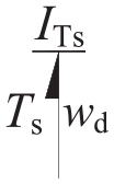
The 2D-EHSPV is designed based on 2D theory, which necessitates the consideration of both linear motion and axial rotation of the spool in the bond graph model. The linear movement of the spool is responsible for controlling the power stage, whereas the axial rotation of the spool serves to regulate the pilot stage. As shown in Figure 5(a), the spool is subjected to viscous friction F_f, inertial force F_s, steady flow force F_sf, transient flow force F_tf, hydraulic spring force F_hs (F_hs = F_sh + F_sp), pilot chamber driving force F_dp and high-pressure chamber driving force F_dh during linear motion. As shown in Figure 5(b), the spool is subjected to viscous friction torque T_f, inertial torque T_s, steady flow torque T_sf, transient flow torque T_tf, and MC drive torque T_d during axial rotation.

Figure 5.

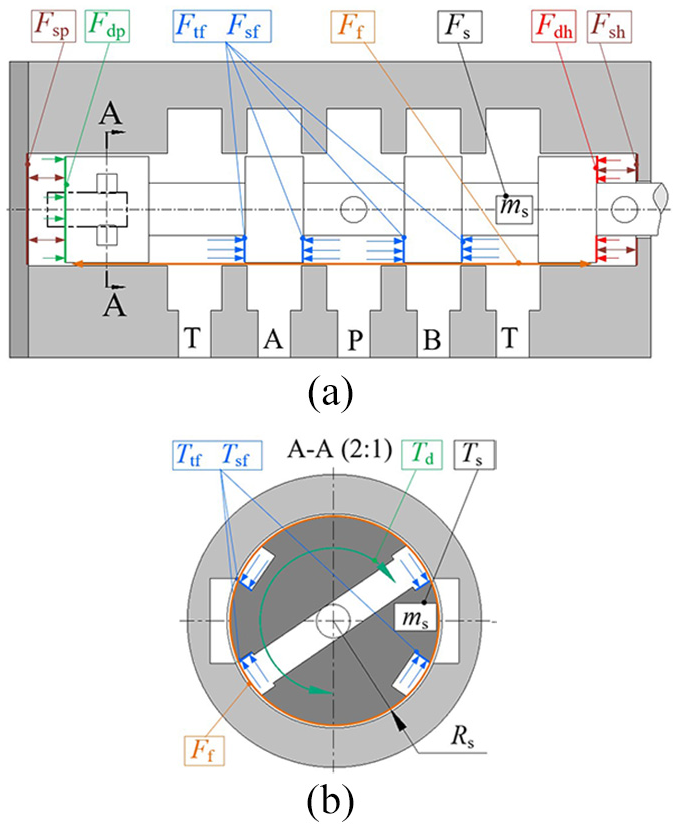
Force/torque diagram of the spool: (a) linear motion and (b) axial rotation.

A bond graph model for the spool’s linear motion was established based on the acting forces, as shown in Figure 6. The input is hydraulic power (pilot stage pressure and flow rate), while the output is mechanical power (spool force and velocity). In this model, R_Ff, R_Fsf, R_Ftf, I_Fs, and C_hs elements at the 1-junction represent viscous friction, steady and transient flow forces, inertial force, and hydraulic spring force, respectively. The pilot and high-pressure chamber driving forces, F_dp and F_dh are generated by chamber pressures acting on the spool’s force areas, with TF elements K_dp and K_hp corresponding to these areas. The equations can be written as:

$$\begin{array}{c}\mathrm{Drive}\mathrm{force}\mathrm{input}\mathrm{Spool},1\mathrm{junction}:\hfill \\ F_{\mathrm{dp}}-F_{\mathrm{dh}}=F_{\mathrm{f}}+F_{\mathrm{tf}}+F_{\mathrm{sf}}+F_{\mathrm{s}}+F_{\mathrm{hs}}\hfill \end{array}$$

(4)

Figure 6.

Bond graph model of the linear motion.

Since the spool’s rotation does not alter chamber volume, no hydraulic spring force is generated. A bond graph model for axial rotation was established based on the acting torques, as shown in Figure 7. Both the input and output are mechanical power, with the input comprising the MC’s torque and angular velocity and the output comprising the spool’s torque and angular velocity. In this model, R_Tf, R_Tsf, R_Ttf, and I_Fs elements at the 1-junction represent viscous friction torque, steady and transient flow torques, and inertial torque, respectively. The equations can be written as:

$$\begin{array}{c}\mathrm{Drive}\mathrm{torque}\mathrm{input}\mathrm{Spool},1\mathrm{junction}:\hfill \\ T_{\mathrm{d}}=T_{\mathrm{f}}+T_{\mathrm{tf}}+T_{\mathrm{sf}}+T_{\mathrm{s}}\hfill \end{array}$$

(5)

Figure 7.

Bond graph model of the axial rotation.

Pilot stage and power stage model

From the perspective of electro-hydraulic servo control, the pilot stage of 2D valve as a three-way rotary valve. Although the pilot and power stages are controlled by spool rotation and direct action, respectively, their hydraulic circuits are interconnected. The oil distribution within the 2D-EHSPV is depicted in Figure 8. In the neutral position, the P- and T-chambers are only connected to the pilot stage, leading to pressure losses in the high-pressure chamber and channel due to oil flow through the PP and PH pipes, which must be represented in the bond graph model. High-pressure oil enters the pilot chamber through the pilot channel at flow rate Q_h, causing a pressure drop to P_c, while the pilot chamber discharges oil to the low-pressure channel at Q_l, further reducing pressure. Spool rotation modulates liquid resistance between the high- and low-pressure channels and the pilot slots, mimicking a three-way rotary valve. During oil flow, the high- and pilot chambers exhibit variable volumes, whereas the high- and low-pressure channels have fixed volumes. When the spool moves away from neutral, the pressure input from the P-chamber to the pilot stage is affected by the A- and B-chambers, whose pressures P_a and P_b depend solely on spool opening in the unloaded state.

Figure 8.

Oil distribution diagram of 2D-EHSPV: (a) power stage and (b) pilot stage.

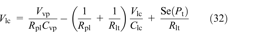
The pilot stage is governed by the pressures P_c in the pilot chamber and P_hc in the high-pressure chamber. P_c originates from the P-chamber and is influenced by throttling effects between the high-, low-pressure, and pilot channels during transmission. Based on the oil distribution diagram, the bond graph model of the pilot stage is established, as shown in Figure 9. Both the input and output are hydraulic power. In the model, elements C_hc, C_vp, and C_lc represent the pressures P_h, P_c, and P_l corresponding to the fixed and variable volumes of the high-pressure, pilot, and low-pressure channels, respectively. Elements R_hp and R_pl represent flow rates Q_hp and Q_hc, which are determined by the opening areas A_h and A_l between the pilot chamber and high-/low-pressure channels. Additionally, C_vh represents P_hc in the high-pressure chamber, corresponding to its variable volume V_vh. The model comprehensively captures the oil flow processes within the pilot stage. The equations can be written as:

$$\mathrm{High}-\mathrm{pressure}\mathrm{channel},0\mathrm{junction}:Q_{\mathrm{pp}}=Q_{\mathrm{hc}}+Q_{\mathrm{hp}}$$

(6)

$$\mathrm{Pilot}\mathrm{chamber},0\mathrm{junction}:Q_{\mathrm{pc}}=Q_{\mathrm{hp}}-Q_{\mathrm{v}}-Q_{\mathrm{pl}}$$

(7)

$$\mathrm{Low}-\mathrm{pressure}\mathrm{channel},0\mathrm{junction}:Q_{\mathrm{lt}}=Q_{\mathrm{pl}}-Q_{\mathrm{lc}}$$

(8)

$$\mathrm{High}-\mathrm{pressure}\mathrm{chamber},0\mathrm{junction}:Q_{\mathrm{hc}}=Q_{\mathrm{ph}}-Q_{\mathrm{vp}}$$

(9)

$$\begin{array}{c}\mathrm{High}-\mathrm{pressure}\mathrm{channel}\mathrm{to}\mathrm{Pilot}\mathrm{chamber},1\mathrm{junction}:\hfill \\ P_{\mathrm{hp}}=P_{\mathrm{h}}-P_{\mathrm{c}}\hfill \end{array}$$

(10)

$$\begin{array}{c}\mathrm{Pilot}\mathrm{chamber}\mathrm{to}\mathrm{Low}-\mathrm{pressure}\mathrm{channel},1\mathrm{junction}:\hfill \\ P_{\mathrm{pl}}=P_{\mathrm{c}}-P_{\mathrm{l}}\hfill \end{array}$$

(11)

Figure 9.

Bond graph model of the pilot stage: (a) pilot chamber and (b) high-pressure chamber.

The power stage of the 2D-EHSPV is an O-type 4/3-way valve with a neutral and two working positions. In the neutral position, the P- and T-chambers connect only to the pilot chamber. When the spool moves along the X-axis, the connections among the P-, T-, A-, and B-chambers change, while the pilot chamber remains linked to the P- and T-chambers. Based on these relationships, a bond graph model of the power stage is established, as shown in Figure 10, primarily illustrating the flow relationships within each oil circuit. The equations can be written as:

$$\begin{array}{c}\mathrm{P}\mathrm{port},0\mathrm{junction}:Q_{\mathrm{p}}=Q_{\mathrm{pa}}+Q_{\mathrm{pb}}+Q_{\mathrm{pp}}+Q_{\mathrm{ph}}\hfill \end{array}$$

(12)

$$\mathrm{T}\mathrm{port},0\mathrm{junction}:Q_{\mathrm{t}}=Q_{\mathrm{at}}+Q_{\mathrm{bt}}+Q_{\mathrm{lt}}$$

(13)

$$\mathrm{A}\mathrm{port},0\mathrm{junction}:Q_{\mathrm{a}}=Q_{\mathrm{pa}}-Q_{\mathrm{at}}$$

(14)

$$\mathrm{B}\mathrm{port},0\mathrm{junction}:Q_{\mathrm{b}}=Q_{\mathrm{pb}}-Q_{\mathrm{bt}}$$

(15)

$$\mathrm{A}\mathrm{port}\mathrm{to}\mathrm{P}\mathrm{port},1\mathrm{junction}:P_{\mathrm{at}}=P_{\mathrm{a}}-P_{\mathrm{t}}$$

(16)

$$\mathrm{P}\mathrm{port}\mathrm{to}\mathrm{A}\mathrm{port},1\mathrm{junction}:P_{\mathrm{pa}}=P_{\mathrm{p}}-P_{\mathrm{a}}$$

(17)

$$\mathrm{P}\mathrm{port}\mathrm{to}\mathrm{B}\mathrm{port},1\mathrm{junction}:P_{\mathrm{pb}}=P_{\mathrm{p}}-P_{\mathrm{b}}$$

(18)

$$\mathrm{B}\mathrm{port}\mathrm{to}\mathrm{T}\mathrm{port},1\mathrm{junction}:P_{\mathrm{bt}}=P_{\mathrm{b}}-P_{\mathrm{t}}$$

(19)

$$\begin{array}{c}\mathrm{P}\mathrm{port}\mathrm{to}\mathrm{High}-\mathrm{pressure}\mathrm{channel},1\mathrm{junction}:\hfill \\ P_{\mathrm{h}}=P_{\mathrm{p}}-P_{\mathrm{pp}}\hfill \end{array}$$

(20)

$$\begin{array}{c}\mathrm{P}\mathrm{port}\mathrm{to}\mathrm{High}-\mathrm{pressure}\mathrm{chamber},1\mathrm{junction}:\hfill \\ P_{\mathrm{ph}}=P_{\mathrm{p}}-P_{\mathrm{hc}}\hfill \end{array}$$

(21)

$$\begin{array}{c}\mathrm{Low}-\mathrm{pressure}\mathrm{channel}\mathrm{to}\mathrm{T}\mathrm{port},1\mathrm{junction}:\hfill \\ P_{\mathrm{lt}}=P_{\mathrm{l}}-P_{\mathrm{t}}\hfill \end{array}$$

(22)

Figure 10.

Bond graph model of the power stage.

Complete model of the 2D-EHSPV

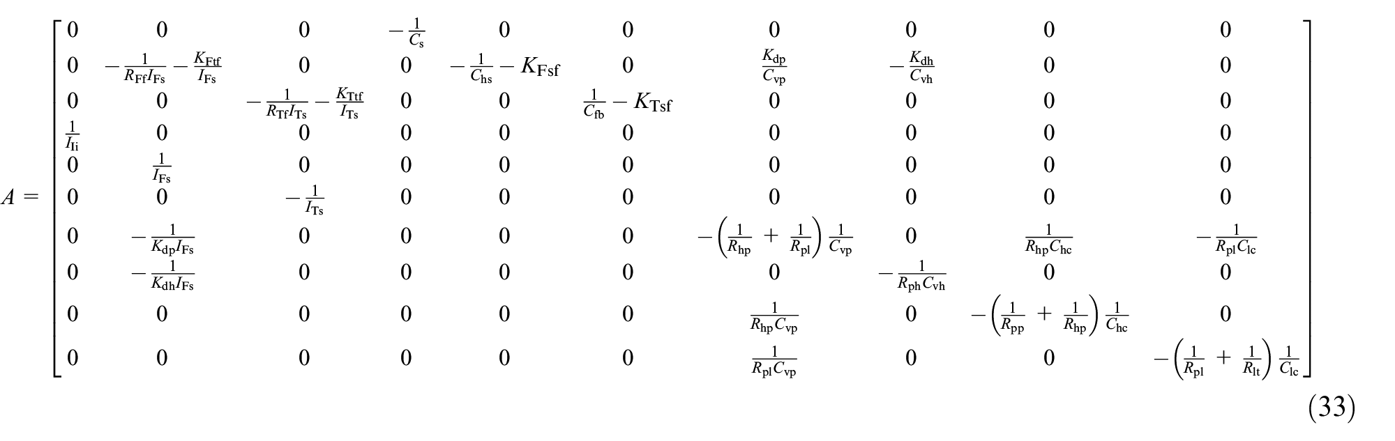
The EMC, MC, spool, pilot stage, and power stage models are integrated based on their structural configurations and power flow directions, forming a complete bond graph model of the 2D-EHSPV, as shown in Figure 11. In this model, R_pl and R_hp are influenced by spool rotation, while C_fb, R_at, R_pa, R_pb, and R_bt are affected by spool movement. The energy storage elements C and I establish derivative or integral relationships, which are used to determine state variables. The relationships between these variables are detailed in Tables 2 and 3.

Figure 11.

Bond graph model of the 2D-EHSPV.

Table 2.

Inertial element.

Bond graph model
Independent variable	F Ii	F s	T s
State variable	E Ii	E s	M s
Equation	$v_{\mathrm{i}}=\frac{E_{\mathrm{Ii}}}{I_{\mathrm{Ii}}}$	$v_{\mathrm{d}}=\frac{E_{\mathrm{s}}}{I_{\mathrm{Fs}}}$	$w_{\mathrm{d}}=\frac{M_{\mathrm{s}}}{I_{\mathrm{Ts}}}$

Table 3.

Capacitive element.

Bond graph model
Independent variable	v ks	v d	w fb	Q vp	Q vh	Q hc	Q lc
State variable	X ks	X d	θ fb	V vp	V vh	V hc	V lc
Equation	$F_{\mathrm{ks}}=\frac{X_{\mathrm{ks}}}{C_{\mathrm{s}}}$	$F_{\mathrm{hs}}=\frac{X_{\mathrm{d}}}{C_{\mathrm{hs}}}$	$T_{\mathrm{d}}=\frac{{\theta }_{\mathrm{fb}}}{C_{\mathrm{fb}}}$	$P_{\mathrm{c}}=\frac{V_{\mathrm{vp}}}{C_{\mathrm{vp}}}$	$P_{\mathrm{vh}}=\frac{V_{\mathrm{vh}}}{C_{\mathrm{vh}}}$	$P_{\mathrm{h}}=\frac{V_{\mathrm{hc}}}{C_{\mathrm{hc}}}$	$P_{\mathrm{l}}=\frac{V_{\mathrm{lc}}}{C_{\mathrm{lc}}}$

State equation

The bond graph model allows the derivation of the state equations for the system, which can be employed in further analyses of the performance of the 2D-EHSPV. The state equation of a system is constituted by a system of first-order differential equations, comprising equations that relate the derivatives between the dependent variables and the corresponding state variables within the system. In accordance with the theory of the bond graph and the interrelationship between the variables, as well as the data presented in Table 2, Table 3, and Figure 11, the state equations can be written as:

$$E_{\mathrm{Ii}}=K_{\mathrm{ps}}\mathrm{Sf}\left(i\right)-\frac{X_{\mathrm{ks}}}{C_{\mathrm{s}}}-K_{\mathrm{mc}}({\theta }_{\mathrm{fb}}+\frac{M_s}{I_{\mathrm{Ts}}})$$

(23)

$$E_{\mathrm{s}}=K_{\mathrm{dp}}\frac{V_{\mathrm{vp}}}{C_{\mathrm{vp}}}-K_{\mathrm{dh}}\frac{V_{\mathrm{vh}}}{C_{\mathrm{vh}}}-\frac{X_{\mathrm{d}}}{C_{\mathrm{hs}}}-\frac{E_{\mathrm{s}}}{R_{\mathrm{Ff}}{I}_{\mathrm{Fs}}}-K_{\mathrm{Fsf}}{X}_{\mathrm{d}}-K_{\mathrm{Ftf}}{X}_{\mathrm{d}}$$

(24)

$$M_{\mathrm{s}}=\frac{{\theta }_{\mathrm{fb}}}{C_{\mathrm{fb}}}-\frac{M_{\mathrm{s}}}{R_{\mathrm{Tf}}{I}_{\mathrm{Ts}}}-K_{\mathrm{Tsf}}{\theta }_{\mathrm{fb}}-K_{\mathrm{Ttf}}{\theta }_{\mathrm{fb}}$$

(25)

$$X_{\mathrm{ks}}=\frac{E_{\mathrm{Ii}}}{I_{\mathrm{Ii}}}$$

(26)

$$X_{\mathrm{d}}=\frac{E_{\mathrm{s}}}{I_{\mathrm{Fs}}}$$

(27)

$${\theta }_{\mathrm{fb}}=K_{\mathrm{mc}}{K}_{\mathrm{ps}}\mathrm{Sf}\left(i\right)-\frac{M_{\mathrm{s}}}{I_{\mathrm{Ts}}}$$

(28)

$$V_{\mathrm{vp}}=\frac{V_{\mathrm{hc}}}{R_{\mathrm{hp}}{C}_{\mathrm{hc}}}-(\frac{1}{R_{\mathrm{hp}}}+\frac{1}{R_{\mathrm{pl}}})\frac{V_{\mathrm{vp}}}{C_{\mathrm{vp}}}-\frac{V_{\mathrm{lc}}}{R_{\mathrm{pl}}{C}_{\mathrm{lc}}}-\frac{E_{\mathrm{s}}}{K_{\mathrm{dp}}{I}_{\mathrm{Fs}}}$$

(29)

$$V_{\mathrm{vh}}=\frac{\mathrm{Se}\left(P_{\mathrm{p}}\right)}{R_{\mathrm{ph}}}-\frac{V_{\mathrm{vh}}}{R_{\mathrm{ph}}{C}_{\mathrm{vh}}}-\frac{E_{\mathrm{s}}}{K_{\mathrm{dh}}{I}_{\mathrm{Fs}}}$$

(30)

$$V_{\mathrm{hc}}=\frac{\mathrm{Se}\left(P_{\mathrm{p}}\right)}{R_{\mathrm{pp}}}-(\frac{1}{R_{\mathrm{pp}}}+\frac{1}{R_{\mathrm{hp}}})\frac{V_{\mathrm{hc}}}{C_{\mathrm{hc}}}+\frac{V_{\mathrm{vp}}}{R_{\mathrm{hp}}{C}_{\mathrm{vp}}}$$

(31)

$$V_{\mathrm{lc}}=\frac{V_{\mathrm{vp}}}{R_{\mathrm{pl}}{C}_{\mathrm{vp}}}-(\frac{1}{R_{\mathrm{pl}}}+\frac{1}{R_{\mathrm{lt}}})\frac{V_{\mathrm{lc}}}{C_{\mathrm{lc}}}+\frac{\mathrm{Se}\left(P_{\mathrm{t}}\right)}{R_{\mathrm{lt}}}$$

(32)

The state model consists of state and output equations. The state equation describes the dynamic relationship between state and input variables, while the output equation defines how the system output depends on state and input variables. The state equations (23)–(32) are reduced to the standard form $X^{.}=\mathrm{AX}+\mathrm{BU}$ , where X is the state vector, U is the input vector. Let us consider the case where the state vector is set to X = [E_Ii, E_s, M_s, X_ks, X_d, θ_fb, V_vp, V_vh, V_hs, V_ls]^T and the input vector is set to U = [Sf(i), Se(Pp), Se(Pt)]^T. In this scenario, the state matrix can be written as:

$$A=\left[\begin{array}{cccccccccc}0\hfill & 0\hfill & 0\hfill & -\frac{1}{C_{\mathrm{s}}}\hfill & 0\hfill & 0\hfill & 0\hfill & 0\hfill & 0\hfill & 0\hfill \\ \multicolumn{1}{c}{0}& -\frac{1}{R_{\mathrm{Ff}}{I}_{\mathrm{Fs}}}-\frac{K_{\mathrm{Ftf}}}{I_{\mathrm{Fs}}}\hfill & 0\hfill & 0\hfill & -\frac{1}{C_{\mathrm{hs}}}-K_{\mathrm{Fsf}}\hfill & 0\hfill & \frac{K_{\mathrm{dp}}}{C_{\mathrm{vp}}}\hfill & -\frac{K_{\mathrm{dh}}}{C_{\mathrm{vh}}}\hfill & 0\hfill & 0\hfill \\ \multicolumn{1}{c}{0}& 0\hfill & -\frac{1}{R_{\mathrm{Tf}}{I}_{\mathrm{Ts}}}-\frac{K_{\mathrm{Ttf}}}{I_{\mathrm{Ts}}}\hfill & 0\hfill & 0\hfill & \frac{1}{C_{\mathrm{fb}}}-K_{\mathrm{Tsf}}\hfill & 0\hfill & 0\hfill & 0\hfill & 0\hfill \\ \multicolumn{1}{c}{\frac{1}{I_{\mathrm{Ii}}}}& 0\hfill & 0\hfill & 0\hfill & 0\hfill & 0\hfill & 0\hfill & 0\hfill & 0\hfill & 0\hfill \\ \multicolumn{1}{c}{0}& \frac{1}{I_{\mathrm{Fs}}}\hfill & 0\hfill & 0\hfill & 0\hfill & 0\hfill & 0\hfill & 0\hfill & 0\hfill & 0\hfill \\ \multicolumn{1}{c}{0}& 0\hfill & -\frac{1}{I_{\mathrm{Ts}}}\hfill & 0\hfill & 0\hfill & 0\hfill & 0\hfill & 0\hfill & 0\hfill & 0\hfill \\ \multicolumn{1}{c}{0}& -\frac{1}{K_{\mathrm{dp}}{I}_{\mathrm{Fs}}}\hfill & 0\hfill & 0\hfill & 0\hfill & 0\hfill & -(\frac{1}{R_{\mathrm{hp}}}+\frac{1}{R_{\mathrm{pl}}})\frac{1}{C_{\mathrm{vp}}}\hfill & 0\hfill & \frac{1}{R_{\mathrm{hp}}{C}_{\mathrm{hc}}}\hfill & -\frac{1}{R_{\mathrm{pl}}{C}_{\mathrm{lc}}}\hfill \\ \multicolumn{1}{c}{0}& -\frac{1}{K_{\mathrm{dh}}{I}_{\mathrm{Fs}}}\hfill & 0\hfill & 0\hfill & 0\hfill & 0\hfill & 0\hfill & -\frac{1}{R_{\mathrm{ph}}{C}_{\mathrm{vh}}}\hfill & 0\hfill & 0\hfill \\ \multicolumn{1}{c}{0}& 0\hfill & 0\hfill & 0\hfill & 0\hfill & 0\hfill & \frac{1}{R_{\mathrm{hp}}{C}_{\mathrm{vp}}}\hfill & 0\hfill & -(\frac{1}{R_{\mathrm{pp}}}+\frac{1}{R_{\mathrm{hp}}})\frac{1}{C_{\mathrm{hc}}}\hfill & 0\hfill \\ \multicolumn{1}{c}{0}& 0\hfill & 0\hfill & 0\hfill & 0\hfill & 0\hfill & \frac{1}{R_{\mathrm{pl}}{C}_{\mathrm{vp}}}\hfill & 0\hfill & 0\hfill & -(\frac{1}{R_{\mathrm{pl}}}+\frac{1}{R_{\mathrm{lt}}})\frac{1}{C_{\mathrm{lc}}}\hfill \end{array}\right]$$

(33)

The input matrix can be written as:

$$B=\left[\begin{array}{ccc}{K}_{\mathrm{ps}}(1-{K_{\mathrm{mc}}}^2)\hfill & 0\hfill & 0\hfill \\ \multicolumn{1}{c}{0}& 0\hfill & 0\hfill \\ \multicolumn{1}{c}{-K_{\mathrm{mc}}{K}_{\mathrm{ps}}{K}_{\mathrm{Ftf}}}& 0\hfill & 0\hfill \\ \multicolumn{1}{c}{0}& 0\hfill & 0\hfill \\ \multicolumn{1}{c}{0}& 0\hfill & 0\hfill \\ \multicolumn{1}{c}{K_{\mathrm{mc}}{K}_{\mathrm{ps}}}& 0\hfill & 0\hfill \\ \multicolumn{1}{c}{0}& 0\hfill & 0\hfill \\ \multicolumn{1}{c}{0}& \frac{1}{R_{\mathrm{ph}}}\hfill & 0\hfill \\ \multicolumn{1}{c}{0}& \frac{1}{R_{\mathrm{pp}}}\hfill & 0\hfill \\ \multicolumn{1}{c}{0}& 0\hfill & \frac{1}{R_{\mathrm{lt}}}\hfill \end{array}\right]$$

(34)

The aim of this paper is to examine the relationship between the input current signal and the spool displacement. Consequently, the output vector Y of the output equation Y = CX + DU can be written as:

$$Y=X_{\mathrm{d}}$$

(35)

The output matrix C can be written as:

$$C=\left[\begin{array}{cccccccccc}0\hfill & 0\hfill & 0\hfill & 0\hfill & 1\hfill & 0\hfill & 0\hfill & 0\hfill & 0\hfill & 0\hfill \end{array}\right]$$

(36)

The direct matrix D can be written as:

$$D=0$$

(37)

Model parameters

The parameters of the bond graph model are derived from the structural characteristics of the 2D-EHSPV. However, there are certain parameters that require additional calculations to be determined.

Torque-displacement coefficient K_mc of the MC

Figure 12 illustrates the magnetic circuit of the MC, which is generated by the permanent magnets on the IM and OM. The permanent magnet material employed in this model is NdFe35. In addition to the magnetic charge surfaces oriented perpendicular to the direction of magnetization, permanent magnets possess inclined magnetic charge surfaces. Nevertheless, the existence of inclined magnetic charge surfaces may lead to complications in the resolution process. In order to facilitate the analytic process and guarantee accuracy, the inclined magnetic charge surface is converted to the magnetic charge surface perpendicular to the magnetizing direction, as shown in Figure 12.

Figure 12.

Magnetic circuit and dimensions of MC.

Based on the law of equivalent magnetic charge,^34,35 the magnetic repulsion between a pair of parallel permanent magnets of unit length can be written as:

$$\mathrm{dF}=\frac{B_1{B}_2}{\pi {\mu }_0{r}_{12}^2}d{s}_{1}d{s}_2$$

(37)

where, B₁ is the residual magnetic of PM1; B₂ is the residual magnetic of PM2; μ₀ is the vacuum magnetic permeability; ds₁ is the per unit area of PM1 microelement; ds₂ is the per unit area of PM2 microelement; r₁₂ is the spacing between ds₁ and ds₂.

Under Figure 12 and equation (37), the integration yields the magnetic repulsion force between a pair of parallel permanent magnets of length l. This magnetic repulsion can be written as:

$$F=\frac{B_1{B}_{2}l}{\pi {\mu }_0}\underset{s_1}{\int }\underset{s_2}{\int }\frac{1}{r_{12}}d{s}_{1}d{s}_2=\frac{B_1{B}_2\mathrm{labcd}}{\pi {\mu }_{0}H(b+H)(b+d+H)}$$

(38)

where, a is the width of PM1; b is the height of PM1; c is the width of PM2; d is the height of PM2; H is the height of the air gap; and l is the length of the two permanent magnets.

The relationship between the input displacement increment Δx of the IM and the air gap height increment ΔH can be written as:

$$\mathrm{\Delta }H=\mathrm{\Delta }{x}_{\mathrm{i}}\cos \beta$$

(39)

where, ΔH is the air gap height increment; Δx_i is the input displacement increment of IM; β is the angle of the MC wing.

The air gap between the permanent magnets can be written as:

$$H_1=H_4=H_0-\mathrm{\Delta }H=H_0-\mathrm{\Delta }{x}_{\mathrm{i}}\cos \beta$$

(40)

$$H_2=H_3=H_0+\mathrm{\Delta }H=H_0+\mathrm{\Delta }{x}_{\mathrm{i}}\cos \beta$$

(41)

where, H₀ is the initial height of the air gap; H_i is the height of the air gap i, i = 1, 2, 3, 4. During the operational phase of the MC, the value of ΔH is less than or equal to H₀.

Combining equations (38), (40), and (41), the equation for the output torque of the MC can be written as:

$$\begin{array}{c}{T}_d=R_{\mathrm{mc}}(F_{\mathrm{ag}1}-F_{\mathrm{ag}2})\sin \beta =\frac{R_{\mathrm{mc}}{B}_1{B}_2\mathrm{labcd}\sin \beta }{\pi {\mu }_0}\hfill \\ (\frac{1}{H_1(b+H_1)(b+d+H_1)}-\frac{1}{H_2(b+H_2)(b+d+H_2)})\hfill \end{array}$$

(42)

where, R_mc is the effective radius of the MC.

Introducing the coefficient M in place of the constant in equation (42), M can be written as:

$$M=\frac{R_{\mathrm{mc}}{B}_1{B}_2\mathrm{labcd}\sin \beta }{\pi {\mu }_0}$$

(43)

From equation (42), it can be observed that the relationship between T_d and x_i is non-linear. The specific parameters were incorporated into equation (42) in order to plot the torque-displacement curve of the MC. The parameters and curve are presented in Table 4. From an examination of the torque-displacement curve, it can be observed that the torque increases exponentially as the magnitude of x_isinβ approaches h₀. In practical working conditions, the value of x_isinβ is typically relatively small, and the expansion of T_d does not exhibit a discernible exponential trajectory. Once T_d has overcome the resisting torque, the value of x_i does not continue to increase. When the displacement of the IM is at 0–1 mm, the torque-displacement curve closely matches the fitted curve with a slope K_mc, although the relationship between torque and displacement is nonlinear. Given that the spool displacement of the 2D-EHSPV is ±1 mm, the slope K_mc of the fitted curve is selected as the torque-displacement coefficient of the MC, which can be employed to reduce the difficulty of calculations.

Table 4.

Torque-displacement curve of MC with specific parameters.

Parameter	Value
Width of PM1, a (mm)	15
Height of PM1, b (mm)	2.5
Width of PM2, c (mm)	12
Height of PM2, d (mm)	5
Length of PMs, l (mm)	15
Length of air gap, H0 (mm)	3
Displacement of IM, xi (mm)	0–1
Radius of magnetic force, Rmc (mm)	15
Angle of the MC wing, β (°)	22
Residual magnetic, B1 = B2 (T)	1.15
Vacuum magnetic permeability, μ0 (H/m)	1.26E-06

Transient and steady flow forces of the spool

The power stage of the 2D-EHSPV is of slide valve construction and is susceptible to significant flow forces at high pressures and flows. Flow forces can be classified into two categories: transient and steady flow forces. Transient flow force is generated as a result of alterations in the valve opening, whereas steady flow force is generated as a result of alterations in the cross-sectional area and direction of the flow. Combining the structure of the slide valve (Figure 13) and the theory of fluid dynamics, the equations for transient flow force F_tf and steady flow force F_sf can be written as:

$$F_{\mathrm{tf}}=\{\begin{array}{c}{C}_{\mathrm{d}}{W}_{\mathrm{s}}{L}_{\mathrm{s}}\sqrt{2\rho P_{\mathrm{pa}}}{X}_{\mathrm{d}}\begin{array}{cc}=K_{\mathrm{Ftf}1}{X}_{\mathrm{d}}\hfill & \mathrm{if}{X}_{\mathrm{d}}>0\hfill \end{array}\hfill \\ \multicolumn{1}{c}{C_{\mathrm{d}}{W}_{\mathrm{s}}{L}_{\mathrm{s}}\sqrt{2\rho P_{\mathrm{pb}}}{X}_{\mathrm{d}}\begin{array}{cc}=K_{\mathrm{Ftf}2}{X}_{\mathrm{d}}\hfill & \mathrm{if}{X}_{\mathrm{d}}<0\hfill \end{array}}\end{array}$$

(44)

$$F_{\mathrm{sf}}=\{\begin{array}{c}2C_{\mathrm{d}}{C}_{\mathrm{v}}{W}_{\mathrm{s}}{P}_{\mathrm{pa}}{X}_{\mathrm{d}}\cos \gamma \begin{array}{cc}=K_{\mathrm{Fsf}1}{X}_{\mathrm{d}}\hfill & \mathrm{if}{X}_{\mathrm{d}}>0\hfill \end{array}\hfill \\ \multicolumn{1}{c}{2C_{\mathrm{d}}{C}_{\mathrm{v}}{W}_{\mathrm{s}}{P}_{\mathrm{pb}}{X}_{\mathrm{d}}\cos \gamma \begin{array}{cc}=K_{\mathrm{Fsf}2}{X}_{\mathrm{d}}\hfill & \mathrm{if}{X}_{\mathrm{d}}<0\hfill \end{array}}\end{array}$$

(45)

where, C_d is the flow coefficient; C_v is the flow velocity coefficient; W_s is the area gradient of the valve port, W_s = 2πR_s;L_s is the distance between valve ports; ρ is the density of the oil; γ is the direction angle of the flow velocity flowing through the valve port.

Figure 13.

Flow diagram of the power stage: (a) X_d > 0 and (b) X_d < 0.

Transient and steady flow torques of the spool

One of the factors that impedes the rotation of the spool is the flow torque. The flow torque is generated by the flow of oil through the high- and low-pressure channels of the spool, as illustrated in Figure 14. When the spool is rotated clockwise through an angle θ with the X axis as the center, the direction of flow from the spool hole through the high-pressure channel into the pilot channel is illustrated in Figure 14(a). Since the pilot channel and the high-pressure channel are parallel to each other, the angle τ between the flow velocity v₆ direction and the YOZ plane is 0. During the rotation of the spool, the opening h_hp of the high-pressure channel in relation to the pilot channel and the opening h_pl of the low-pressure channel in relation to the pilot channel are always greater than zero. Consequently, the direction of the flow torque remains unaltered. In accordance with the fluid flow model at the pilot stage illustrated in Figure 14, the equations for the transient flow torque and steady flow torque can be written as:

$$T_{\mathrm{tf}}=C_{\mathrm{d}}{A}_{\mathrm{h}}{R}_{\mathrm{s}}\sqrt{2\rho P_{\mathrm{hp}}}\theta =K_{\mathrm{Ttf}}\theta$$

(46)

$$T_{\mathrm{sf}}=2C_{\mathrm{d}}{C}_{\mathrm{v}}{W}_{\mathrm{h}}{R}_{\mathrm{s}}{P}_{\mathrm{hp}}\theta \cos \tau \cos {\tau }_{\mathrm{o}}=K_{\mathrm{Tsf}}\theta$$

(47)

where, W_h is the area gradient of the high-pressure channel; R_s is the radius of the spool; P_hp is the differential pressure between the high-pressure channel and the pilot channel; θ is the rotational angle of the spool; τ is the angle between the v₆ direction and the YOZ plane; τ_o is the angle between the v₆ direction and the XOY plane.

Figure 14.

Flow diagram of the pilot stage: (a) direction of flow in high-pressure channel and (b) sectional view at section A.

Flow rate of the pilot stage

The flow rate Q_hp from the high-pressure channel into the pilot channel is calculated by the following equation:

$$Q_{\mathrm{hp}}=C_{\mathrm{d}}{A}_{\mathrm{h}}\sqrt{\frac{2P_{\mathrm{hp}}}{\rho }}$$

(48)

where, A_h is the opening area of the high-pressure channel.

The flow rate Q_pl from the pilot channel into the low-pressure channel is calculated by the following equation:

$$Q_{\mathrm{pl}}=C_{\mathrm{d}}{A}_{\mathrm{h}}\sqrt{\frac{2P_{\mathrm{pl}}}{\rho }}$$

(49)

where, A_l is the opening area of the low-pressure channel; P_pl is the differential pressure between the low-pressure channel and the pilot channel.

The areas A_h and A_l are subject to change as a result of the rotation of the spool, as shown in Figure 15. In operational conditions, the only applicable range for h is 0 ≤ h < r. Consequently, the equations of A_h and A_l can be written as:

$$A_{\mathrm{h}}=r^2\arccos \left(\frac{r-h_{\mathrm{hp}}}{r}\right)+w{h}_{\mathrm{hp}}-(r-h_{\mathrm{hp}})\sqrt{r^2-{(r-h_{\mathrm{hp}})}^2}$$

(50)

$$A_{\mathrm{l}}=r^2\arccos \left(\frac{r-h_{\mathrm{pl}}}{r}\right)+w{h}_{\mathrm{pl}}-(r-h_{\mathrm{pl}})\sqrt{r^2-{(r-h_{\mathrm{pl}})}^2}$$

(51)

where, r is the chamfer radius of the high- and low-pressure channels; w is the width of high- and low-pressure channels; h_hp is the opening of the high-pressure channel in relation to the pilot channel; h_pl is the opening of the low-pressure channel in relation to the pilot channel.

Figure 15.

Opening diagrams of pilot stage at different rotation angle: (a) h = 0, (b) 0 ≤ h < r, (c) r ≤ h < l, and (d) l ≤ h < H_p.

The h_hp and h_pl can be written as:

$$h_{\mathrm{hp}}=h_0+\mathrm{\Delta }h$$

(52)

$$h_{\mathrm{pl}}=h_0-\mathrm{\Delta }h$$

(53)

As a consequence of the magnetic constraint and displacement feedback of the MC, the value of Δh is dependent upon both the input displacement Δx_i of the EMC and the output displacement Δx_o of the MC. The following relationship exists between Δh, Δx_i, and Δx_o:

$$\mathrm{\Delta }h=\frac{R_{\mathrm{s}}(\mathrm{\Delta }{x}_{\mathrm{i}}-\mathrm{\Delta }{x}_{\mathrm{o}})\tan \beta }{R_{\mathrm{mc}}}$$

(54)

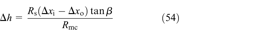
where, R_s is the radius of the spool.

Remaining parameters in the model

In addition to the previously detailed flow and torque coefficients, namely the transient and steady state flow force coefficients (K_Ftf, K_Fsf), the transient and steady state flow torque coefficients (K_Ttf, K_Tsf), and the conversion coefficient of the magnetic converter K_mc, this section presents the derivation and calculation of the remaining key parameters required for accurate modeling of the 2D-EHSPV. These parameters primarily pertain to internal resistances, stiffness characteristics, and fluid capacities that critically influence the dynamic response of the valve system.

Specifically, the viscous resistance forces and torques acting on the spool, denoted as F_f and T_f, are calculated based on classical laminar shear theory, considering the annular gap geometry and dynamic viscosity of the working fluid. The equations of F_f and T_f can be written as:

$$F_{\mathrm{f}}=\mu \frac{A_{\mathrm{s}}{v}_{\mathrm{d}}}{\delta }=R_{\mathrm{Ff}}{v}_{\mathrm{d}}$$

(55)

$$T_{\mathrm{f}}=\mu \frac{2\pi R_{\mathrm{s}}^3{L}_{\mathrm{v}}{w}_{\mathrm{d}}}{\delta }=R_{\mathrm{Tf}}{w}_{\mathrm{d}}$$

(56)

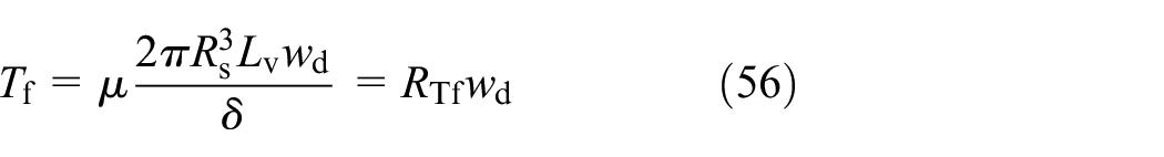
where, A_s is the cylindrical lateral surface area of the spool wetted by the hydraulic fluid; μ is the fluid viscosity coefficient; L is the effective length of viscous force application; δ is the radial clearance between the spool and sleeve.

The flow resistances between chambers, including the resistance from the P chamber to the high-pressure chamber R_ph, from the P chamber to the pilot chamber R_pp, and from the low-pressure channel to the T chamber R_lt, are determined using standard orifice flow models that incorporate geometric parameters and discharge coefficients. The equations of R_ph, R_pp, and R_lt can be written as:

$$R_{\mathrm{ph}}=\frac{128\mu L_{\mathrm{ph}}}{\pi D^4}$$

(57)

$$R_{\mathrm{pp}}=\frac{128\mu L_{\mathrm{pp}}}{\pi D^4}$$

(58)

$$R_{\mathrm{lt}}=\frac{128\mu L_{\mathrm{lt}}}{\pi D^4}$$

(59)

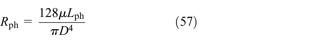
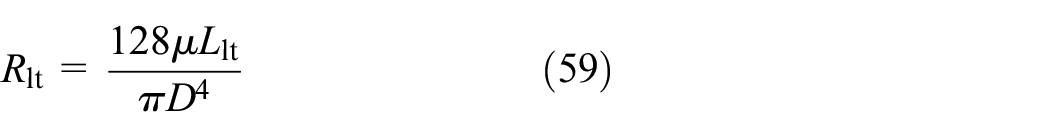
where, L_ph is the length from the P chamber to the high-pressure chamber; L_pp is the length from the P chamber to the pilot chamber; L_lt is the length from the low-pressure channel to the T chamber; D is the flow channel diameter.

The hydraulic spring compliance C_hs, which arises from the compressibility of the fluid in confined chambers, is derived from the bulk modulus and effective fluid volume. The equations of C_hs can be written as:

$$C_{\mathrm{hs}}={(\frac{{\beta }_{\mathrm{e}}{A_{\mathrm{p}}}^2}{V_{\mathrm{p}}}+\frac{{\beta }_{\mathrm{e}}{A_{\mathrm{h}}}^2}{V_{\mathrm{h}}})}^{-1}$$

(60)

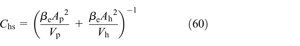
where, A_p is the force area of the spool in the pilot chamber; A_h is the force area of the spool in the high-pressure chamber; V_p is the volume of the pilot chamber; V_h is the volume of the high-pressure chamber.

The magnetic feedback compliance C_fb is determined by the magnetic circuit parameters of MC, based on the torque-angle relationship under small perturbations. The equations of C_fb can be written as:

$$C_{\mathrm{fb}}=\frac{1}{K_{\mathrm{mc}}}$$

(61)

where, K_mc is the conversion coefficient of MC.

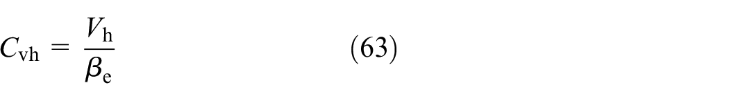
The fluid capacities of the pilot chamber C_vp and high-pressure chamber C_vh are defined as the ratio of the chamber volume to the fluid bulk modulus, reflecting their capacity to store and transmit pressure variations. The equations of C_vp and C_vh can be written as:

$$C_{\mathrm{vp}}=\frac{V_{\mathrm{p}}}{{\beta }_{\mathrm{e}}}$$

(62)

$$C_{\mathrm{vh}}=\frac{V_{\mathrm{h}}}{{\beta }_{\mathrm{e}}}$$

(63)

Experimental validations

To verify the accuracy and applicability of the proposed bond graph model, all simulations in this study were conducted using Matlab/Simulink, and the results were compared with corresponding experimental data obtained from a physical prototype of the 2D-EHSPV. The structural parameters and material properties of the valve, which serve as key inputs to the bond graph model, are summarized in Table 5. These parameters were not arbitrarily selected; instead, they were determined based on established design principles and guided by relevant literature. Specifically, reference was made to previous studies,^7,13,14 ensuring that the selected values align with validated configurations reported in the field. Additionally, to guarantee system stability under dynamic conditions, the parameter values were cross-validated against the resonance stability criterion introduced in Xu et al., ¹² which offers a theoretical basis for appropriately balancing mass, damping, and stiffness. These considerations ensure that the adopted parameters reflect both theoretical rigor and practical feasibility. Furthermore, Table 6 lists the simulation parameters used in the bond graph model, which were derived analytically from the structural data in Table 5 using the equations detailed in Section “Model parameters.” These include the calculation of inertial, compliant, and resistive elements (I, C, and R elements) in accordance with the bond graph methodology. This structured approach enables a faithful representation of the nonlinear, multi-energy-domain interactions inherent in 2D-EHSPV systems, thereby enhancing the physical realism and predictive accuracy of the simulation model.

Table 5.

Parameters of the 2D-EHSPV.

Components	Parameters	Value
EMC	Coil voltage Ui (V)	24
	Coil resistance Rc (Ω)	20
MC	Pitch angle of MC β (°)	22
	Radius of magnetic force Rmc (mm)	15
	Mass of IM mIM (kg)	0.2
	Mass of OM mOM (kg)	0.2
	Dimensions of PM1 (a × b × l) (mm)	15 × 2.5 × 15
	Dimensions of PM2 (c × d × l) (mm)	12 × 5 × 15
	Initial height of air gap H0 (mm)	2.8, 3, 3.2
Pilot stage	Initial height of overlapping area h0 (mm)	0.2
	Initial length of pilot chamber (mm)	4
	Initial length of high-pressure chamber Lh (mm)	3
	Length from P chamber to high-pressure chamber Lph (mm)	36
	Length from P chamber to pilot chamber Lpp (mm)	36
	Length from low-pressure channel to T chamber Llt (mm)	15
	Width of high- and low-pressure channels w (mm)	3
	Angle between v6 and YOZ plane τ (°)	6
	Angle between v6 and XOY plane τ0 (°)	38
	Chamfer radius of high- and low-pressure channels r (mm)	0.5
	Flow channel diameter D (mm)	3
Power stage	Radius of spool land Rs (mm)	9
	Radius of spool rod Rsr (mm)	4
	Mass of spool ms (kg)	0.5
	Angle of flow γ (°)	69
	Distance between valve ports Ls (mm)	21
	Effective length of viscous force application Ly (mm)	45
	Radial clearance between spool and sleeve δ (mm)	0.019
Other	Residual magnetic of NdFe35 B/T	1.15
	Vacuum magnetic permeability μ0 (H/m)	1.26E-06
	Oil density ρ (kg/m3)	850
	Elasticity of bulk modulus βe (MPa)	700
	Flow rate coefficient Cd	0.61
	Flow velocity coefficient Cv	0.98
	Fluid viscosity coefficient μ kg/(m s)	0.034

Table 6.

Elements of the bond graph model.

Elements	Value	Elements	Value
Viscous resistance coefficient (force) RFf (N s/m)	4.6	Mass of the OM and the spool IFs or ITs (kg)	0.7
Transient flow force coefficient RFtf (N s/m)	1.3E+03	Mechanical spring compliance Cs (m/N)	5E-05
Steady flow force coefficient RFsf (N s/m)	4.4E+05	Hydraulic spring compliance Chs (m/N)	1.1E-08
Viscous resistance coefficient (torque) RTf (Nm s/rad)	3.7E-04	Magnetic feedback compliance Cfb (rad/Nm)	2.4E-03
Transient flow torque coefficient RTtf (Nm s/rad)	1.5E-02	Fluid capacities of the pilot chamber Cvp (m5/N)	1.5E-15
Steady flow torque coefficient RTsf (Nm s/rad)	6.1E+02	Fluid capacities of the high-pressure chamber Cvh (m5/N)	8.8E-16
Fluid resistance from the P-chamber to the high-pressure chamber Rph (Pa s/m3)	6.2E+08	Current-force coefficient of EMC Kps (N/A)	6E+01
Fluid resistance from the P-chamber to the pilot chamber Rpp (Pa s/m3)	6.2E+08	Conversion coefficient of MC Kmc (Nm/m)	4.2E+02
Fluid resistance from the low-pressure channel to the T-chamber Rlt (Pa s/m3)	2.6E+08	Force area of the pilot chamber Kp (m2)	2.5E-04
Mass of the IM and the EMC armature IIi (kg)	0.25	Force area of high-pressure chamber Kh (m2)	1.9E-04

Accuracy of MC analytical model

The MC is the key component of the 2D-EHSPV for thrust-torque conversion and displacement feedback. It is therefore necessary to verify the analytical model of the MC before proceeding with the simulation of the bond graph model. A prototype of the MC was manufactured in accordance with the dimensional parameters specified in Table 5. Given that equation (42) expresses the torque-displacement characteristics of the MC, only static experiments of the MC are required in this paper. Figure 16 illustrates the static experimental platform of MC, which primarily comprises the MC prototype, voice coil motor (VCM), torque sensor, oscilloscope, laser displacement sensor, springs, bearings, and other fixed components. During the static experiment, the voice coil motor drove the IM to move axially, the torque sensor measured the output torque of the OM, the laser displacement sensor measured the input displacement of the IM, and the oscilloscope recorded all the data.

Figure 16.

Static experimental platform of MC: (a) schematic diagram and (b) physical diagram.

Figure 17 illustrates the torque-displacement curves of the MC at H₀ of 2.8, 3, and 3.2 mm. The blue, black, and red lines represent the experimental results, analytical results, and fitted results, respectively. It can be observed that all curves demonstrate an increasing trend with increasing displacement x_i. The experimental maximum output torque is 0.32, 0.4, and 0.47 Nm, while the analytical maximum output torque is 0.35, 0.42, and 0.48 Nm, respectively. This indicating a minor discrepancy between the two results. Furthermore, both the experimental and analytical curves are nonlinear and in good agreement. This verifies the accuracy of the model. The experimental results are slightly smaller than the analytical results for the following reasons: (1) The material properties in the calculations are different to reality; (2) The nonlinearity of the permeability is not taken into account in the analytical model; (3) The magnetic energy of permanent magnets is lost during assembly.

Figure 17.

Torque-displacement curves of MC: (a) H₀ = 2.8 mm, (b) H₀ = 3 mm, and (c) H₀ = 3.2 mm.

Accuracy of bond graph model

The accuracy of the bond graph model is verified by comparing analytical results with experimental data. The model analysis is conducted using Matlab/Simulink, where the state equation derived from the bond graph model involves ten variables, increasing computational complexity. To analyze the dynamic behavior of complex systems, this paper employs Matlab/Simulink for bond graph model simulation. Utilizing Simulink’s graphical interface and module library, an accurate simulation model of the 2D-EHSPV was developed based on equations (33)–(37). Furthermore, based on the dimensional parameters in Table 4, a 3D model of the 2D-EHSPV was designed, and the corresponding experimental prototype was manufactured, as shown in Figure 18.

Figure 18.

Prototype of 2D-EHSPV.

Figure 19 shows the built experimental platform, together with the corresponding hydraulic schematic. The experimental platform comprises a variety of components, including 2D-EHSPV, pump, relief valve, throttle valve, signal generator, proportional amplifier, laser displacement sensor, oscilloscope, pressure gauge, and flow meter. The experimental platform is capable of conducting hydraulic experiments with a maximum pressure of 35 MPa.

Figure 19.

Experimental platform of 2D-EHSPV.

According to electro-hydraulic servo control theory, the static characteristics of a mechanical-hydraulic control system depend on manufacturing and assembly, while its dynamic characteristics are primarily influenced by structural parameters. Since manufacturing and assembly errors are not considered in the bond graph model, this paper focuses on dynamic experiments of the 2D-EHSPV to compare with the model’s simulation results. Step response and frequency response experiments were conducted to validate the model’s accuracy in representing the dynamic characteristics of the 2D-EHSPV.

The step response curve is shown in Figure 20, with attention paid to the step rise time and curve characteristics. The experimental and analytical results are shown in Table 7. The maximum relative error in step response time is 6.25%, indicating good agreement between the analytical predictions and experimental data. The absence of overshoot in both the experimental and analytical curves indicates that the 2D EHSPV is an overdamped system at this parameter and has good operational stability.

Figure 20.

Step response curves of 2D-EHSPV: (a) 4 MPa, (b) 8 MPa, and (c) 16 MPa.

Table 7.

Step response time of 2D-EHSPV.

P s (MPa)	4	8	16
Experimental tr (ms)	136	112	80
Analytical tr (ms)	128	105	76
Relative error (%)	5.88	6.25	5.00

The frequency response curves of the 2D-EHSPV are shown in Figure 21, which depicts the amplitude-frequency and phase-frequency characteristics at 16 MPa, respectively. Experimental and analytical results consistently demonstrate that, at low frequencies, the spool displacement closely follows the input signal. From the sinusoidal responses at 0.1, 10, and 30 Hz, it is evident that as the input frequency increases, the output amplitude decreases while the phase lag between input and output signals becomes more pronounced. The experimentally measured amplitude and phase bandwidths of the 2D-EHSPV at 16 MPa are 22.8 and 32.6 Hz, respectively, whereas the corresponding analytical values are 24.2 and 34.5 Hz. The maximum relative errors between analytical predictions and experimental data are 6.14% in terms of the frequency response characteristics, indicating a good agreement between the model and experimental observations. Furthermore, although the intrinsic frequency response of the 2D valve body exceeds 200 Hz, ³⁶ the lower overall frequency response of the 2D-EHSPV is primarily limited by EMC. This limiting effect is also reflected in the frequency response results obtained from the bond graph model.

Figure 21.

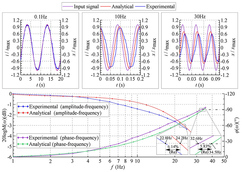
Frequency response curves of 2D-EHSPV.

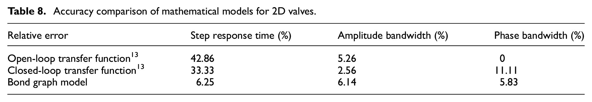
To further evaluate the modeling accuracy, a comparative analysis is conducted between the bond graph based mathematical model proposed in this study and the model presented in Zheng et al., ¹³ which is the only one among the cited works^7,13,14 that has undergone experimental validation. Table 8 presents a comparative analysis of the relative errors in key dynamic performance indicators, including step response time, amplitude bandwidth, and phase bandwidth. First, the relative error in step response time is significantly higher in the linear models derived from Zheng et al., ¹³ with 42.86% for the open-loop and 33.33% for the closed-loop configurations. This suggests that linear models are particularly inadequate in capturing the transient dynamics of the system, likely due to their inability to represent nonlinear damping and inertia effects during rapid signal changes. Second, while the open-loop transfer function model surprisingly shows zero error in phase bandwidth, this result is likely coincidental and does not reflect overall modeling fidelity, as it fails to account for the large errors observed in other performance metrics. Moreover, the closed-loop model, though slightly better in amplitude bandwidth prediction (2.56%), suffers from a notable 11.11% error in phase bandwidth, indicating inconsistencies in dynamic behavior prediction across the frequency domain. In contrast, the bond graph model not only delivers significantly lower errors in all three categories but also maintains a balanced accuracy across both time-domain (step response) and frequency-domain (amplitude and phase bandwidth) indicators. This consistency highlights the robustness of the bond graph methodology in modeling cross-domain energy interactions and nonlinear effects typical of 2D electro-hydraulic systems. Furthermore, the bond graph model avoids the overfitting or over-simplification tendencies commonly observed in linearized models, thereby offering a more physically grounded and generalizable framework suitable for a wide range of operating conditions. These findings reinforce the conclusion that the bond graph approach provides a substantial advancement in the precision modeling of 2D valve dynamics, which is critical for the development of high-performance control strategies in electro-hydraulic applications.

Table 8.

Accuracy comparison of mathematical models for 2D valves.

Relative error	Step response time (%)	Amplitude bandwidth (%)	Phase bandwidth (%)
Open-loop transfer function 13	42.86	5.26	0
Closed-loop transfer function 13	33.33	2.56	11.11
Bond graph model	6.25	6.14	5.83

A closer examination of the residual discrepancies between the analytical predictions of the bond graph model and the experimental measurements reveals that these errors, although significantly lower than those associated with conventional linear models, are not negligible and can be primarily attributed to two key sources. First, the physical prototype of 2D-EHSPV inevitably exhibits manufacturing and assembly imperfections, such as spool misalignment, uneven clearances, and surface roughness, which alter internal flow dynamics and introduce unmodeled parasitic effects such as additional damping or friction. These physical deviations, although minor in magnitude, can contribute up relative error in dynamic response characteristics, particularly affecting parameters like step response time and steady-state displacement accuracy. ³⁷ Second, EMC serves as the core actuator, is susceptible to thermal degradation under high-frequency excitation. This thermal effect leads to decreased magnetic permeability and actuator efficiency, thereby causing reduced output force and dynamic performance deterioration, which contributes an additional relative error in amplitude and phase bandwidth predictions. ³⁸ Although the bond graph modeling approach significantly enhances predictive accuracy by capturing the nonlinear, multi-domain dynamics of the 2D valve system, these unmodeled practical influences underscore the necessity of incorporating thermal effects and manufacturing tolerances into future model refinements to further improve simulation fidelity.

Simulation

The performance of the 2D EHSPV is determined by both manufacturing precision and critical structural parameters. The static characteristics, including steady-state displacement accuracy and internal leakage, are particularly sensitive to the machining accuracy of individual components and potential assembly misalignments, which may alter internal flow dynamics and compromise overall performance. In contrast, the dynamic characteristics are predominantly influenced by the structural configuration of the magnetic circuit and the pilot stage. Key factors include component mass, inherent damping properties, electromagnetic force generation, and geometric features of the flow channels. In the present section, a comprehensive analysis of the static and dynamic characteristics of the 2D EHSPV is conducted based on the bond graph model, which has been previously validated through comparison with experimental data. The overarching objective is to identify strategies that enhance system stability, improve energy conversion efficiency, and increase feedback precision.

Stability

A reduction in the stability of the 2D-EHSPV can lead to fluctuations in flow or pressure, potentially causing vibrations, noise, or even system failure. The bond graph model clearly illustrates that both the MC and the pilot stage directly influence the power stage. From equations (43) and (54), it is evident that β has a significant effect on the torque-pressure characteristics of the MC. Similarly, equations (50) and (51) show that w directly impacts the flow gain of the control stage. Consequently, β and w have been chosen for investigation to assess their influence on the stability of the 2D-EHSPV. Based on the structural characteristics of the MC, the maximum value of β is limited to 90°, as depicted in Figure 2. Regarding the spool structure, the maximum value of w is restricted to the length of the spool shoulder (10 mm), as shown in Figure 15. Apart from β and w, the remaining parameters are set according to Tables 5 and 6. The Nyquist diagram in Figure 22 was obtained through simulation. As seen in Figure 22(a), the radius of the Nyquist diagram gradually increases as β rises, with the graph shifting closer to the positive side of the real axis. This indicates a faster system response. However, if the curve encircles the −1 point more frequently, this may compromise the system’s stability. Additionally, as β increases, the system experiences greater phase lag, causing the graph to deviate more significantly from the origin and approach the −1 point. In summary, increasing β causes the Nyquist diagram to expand and move closer to the −1 point, which could lead to system instability. When β reaches 67°, the curve intersects the −1 point, marking the critical stability threshold for this set of parameters. From Figure 22(b), it is apparent that w exerts a similar effect on system stability as β, though it is more conservative and better suited for fine-tuning the system’s performance. When w reaches 10 mm, the system remains stable, but overshoot and oscillations begin to occur, affecting system performance to a certain extent.

Figure 22.

Nyquist diagram of 2D-EHSPV: (a) β and (b) w.

In conclusion, increasing β and w enhances the gain of the system, but care should be taken to avoid overdoing it, which leads to a decrease in stability. Under the parameter constraints specified in Tables 5 and 6, β should not exceed 67°. By adjusting these two parameters, it is possible to identify a combination that ensures the desired response speed while maintaining the stability of 2D-EHSPV.

Energy efficiency

The steady flow torque of the pilot stage represents the primary impediment to the rotation of the spool and determines the input power of the EMC. Consequently, an investigation into this phenomenon can facilitate improvements in the driving efficiency of the entire valve, thereby achieving the objective of energy conservation. The 2D valve spool exhibits a small turning angle, typically within the range of ±1.44°. ³⁶ This paper investigates the effect of h_o (0.2, 0.25, 0.3, 0.35 mm) and r (0.5, 0.6, 0.7, 0.8 mm) on the steady flow torque of the pilot stage at an angle of ±1.44°. The parameters delineated in this section are set in accordance with the specifications outlined in Tables 5 and 6, with the exception of h₀ and r, which are set as variables. The simulation results are shown in Figure 23, and the maximum steady flow torque within the specified angle interval are shown in Table 9. From Figure 23(a), it can be seen that the growth of the steady flow torque shows a clear positive correlation with h₀, and the maximum steady flow torque corresponding to h₀ of 0.2, 0.25, 0.3, and 0.35 mm are 0.283, 0.334, 0.385, and 0.437 Nm, respectively. From Figure 23(b), the growth of the steady flow torque exhibits a nonlinear relationship with r, and the maximum steady flow torque corresponding to r of 0.5, 0.6, 0.7, and 0.8 mm are 0.144, 0.283, 0.350, and 0.379 Nm, respectively. In addition, a comparison of the slopes of the curves shows that the effect of turning angle on the steady flow torque becomes increasingly pronounced as r increases.

Figure 23.

Torque-angle curves of 2D-EHSPV: (a) h₀ and (b) r.

Table 9.

Maximum steady flow torque.

h 0 (mm)	T sf (Nm)	r (mm)	T sf (Nm)
0.2	0.283	0.5	0.144
0.25	0.334	0.6	0.283
0.3	0.385	0.7	0.350
0.35	0.437	0.8	0.379

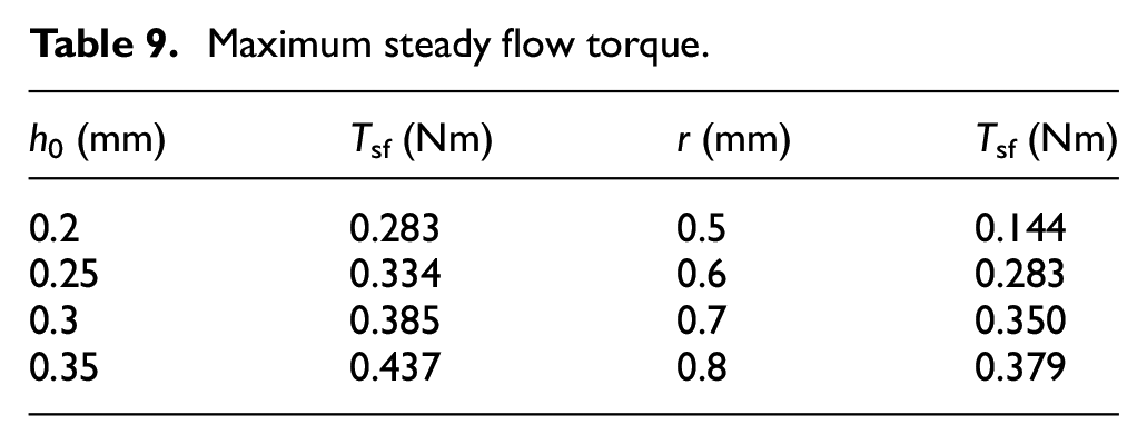
In conclusion, h₀ represents the initial opening of the pilot stage and r represents the flow area gradient of the pilot stage. Both of these variables are positively correlated with the steady flow torque of the pilot stage. The energy efficiency of the EMC can be improved by reducing h₀ and r to reduce the steady flow torque when the dynamic characteristics of 2D-EHSPV meet the design requirements.

Feedback accuracy

The feedback accuracy affects the flow regulation of the 2D-EHSPV. In this section, the feedback accuracy of the 2D-EHSPV is determined by analyzing the steady-state error of the step response curve. Given that H₀ and L_pc are readily adjustable and exert an influence on the system stiffness, the impact of H₀ (2.8, 3, 3.2, 3.4 mm) and L_pc (2.5, 3, 3.5, 4 mm) on the feedback accuracy of 2D-EHSPV is examined. The parameters were set in accordance with the specifications outlined in Tables 5 and 6, with the exception of H₀ and L_pc, which were designated as variables. The step response curves are shown in Figure 24, and a summary of the step rise times and steady-state errors is presented in Table 10. From Figure 24(a), the final output displacement of spool is 1 mm, exhibiting a tendency toward stabilization over time. The enlarged section illustrates that the stable spool displacements for H₀ of 3.4, 3.2, 3, and 2.8 mm are 0.998, 1.004, 1.009, and 1.012 mm, respectively. It can be observed that as H₀ decreases, the steady-state error decreases and then increases, while the step response continues to become faster. On the other hand, the impact of H₀ on the steady-state error is reduced as its value decreases. Figure 24(b) illustrates that the stable spool displacements for L_pc of 4, 3.5, 3, and 2.5 mm are 1.012, 1.016, 1.018, and 1.019 mm, respectively. In addition, it can be observed that a reduction in L_pc results in an increase in the steady-state error, while the step response time remains unaltered.

Figure 24.

Step response curves of 2D-EHSPV: (a) H₀ and (b) L_pc.

Table 10.

The step rise times and steady-state errors of 2D-EHSPV.

H 0 (mm)	t r (ms)	E s (%)	L pc (mm)	t r (ms)	E s (%)
3.4	109	−0.2	4	73	1.2
3.2	93	0.4	3.5	73	1.6
3	81	0.9	3	73	1.8
2.8	73	1.2	3.5	73	1.9

In conclusion, H₀ represents the permanent magnet stiffness of MC, which is positively correlated with the feedback accuracy. Therefore, the larger the value of H₀, the better the feedback accuracy will be, provided that the stroke and power-to-weight ratio satisfy the design requirements. L_pc represents the initial volume of the pilot stage, which is positively correlated with the feedback accuracy, but does not affect the step response speed. Therefore, L_pc can be appropriately enlarged if the power-to-weight ratio is not constrained.

Conclusions

1. A bond graph model of the 2D-EHSPV was developed following a detailed analysis of key nonlinear factors that influence system, including magnetic hysteresis, Coulomb friction, and flow force. The bond graph model concretely illustrates the energy transfer relationships among the electro-mechanical converter (EMC), magnetic levitation coupling (MC), and the 2D valve body, exemplifying the working principle of a two-dimensional pilot. Each of these components plays a crucial role in simulating the dynamics of the 2D-EHSPV, allowing for a precise representation of its response under various operating conditions. This modular structure not only enhances the clarity and flexibility of the model but also provides a comprehensive foundation for in-depth performance analysis and subsequent optimization of the valve design.

2. A Matlab/Simulink simulation model was constructed based on the bond graph model of 2D-EHSPV. The simulation results are in good agreement with the experimental results in terms of static and dynamic characteristics (the maximum relative error is 6.25%), which indicates that the bond graph model can provide a reliable theoretical foundation for 2D-EHSPV design.

3. The effects of key structural parameters on the stability, energy efficiency, and feedback accuracy of the 2D EHSPV are investigated using a validated Matlab/Simulink simulation model. The gain of the MC and pilot stage is negatively correlated with the stability, and the relationship between response speed and stability requires balancing multiple sets of parameters. The flow area gradient of the pilot stage is positively correlated with steady flow force; it should be reduced to improve energy efficiency while ensuring adequate pressure gain. The permanent magnet stiffness of the MC is positively correlated with feedback accuracy and should be increased as much as the stroke and power-to-weight ratio allow. The initial volume of the pilot stage is positively correlated with the feedback accuracy, but does not affect the step response speed. Building on these findings, future work could involve multi-objective optimization by assigning different weights to performance targets, enabling the development of 2D-EHSPVs that satisfy various performance criteria, such as low power consumption with high dynamic response, high flow with high dynamic response, and high flow with a high power-to-weight ratio, among others.

4. While the present study primarily emphasizes the short-term dynamic accuracy of the 2D electro-hydraulic servo proportional valve under nominal conditions, the long-term reliability and performance degradation under extended operational stress remain critical aspects for real-world applications. Factors such as component wear, material fatigue, seal aging, and thermal effects on EMC may cumulatively affect system stability and precision. These aspects were not addressed in the current work but will be considered in future studies, which will incorporate thermal-mechanical coupling, aging models, and long-term durability testing to further enhance the robustness and applicability of the proposed modeling approach.