
Abstract
Digital twins (DT) represent a groundbreaking advancement in industrial process management. They serve as faithful virtual replicas of a physical process or equipment, enabling a comprehensive understanding of its real-time behavior. These duplicates evolve over time in synchronization with the physical twin, being updated at a frequency and precision appropriate to the monitored issue. This article aims to develop a DT for monitoring fatigue damage in Pressure Vessels (PVs). This DT relies on the integration of several innovative technologies like Internet of Things (IoT) and simulation. IoT facilitates data transmission to the DT for real-time monitoring and continuous acquisition of the physical state. Integrated simulation provides a precise representation of the behavior of the physical vessel. To this end, a Finite Element (FE) numerical model is developed to simulate the mechanical behavior of the equipment under cyclic loading. This model is validated using experimental data obtained from inspections and instrumentation conducted on the PV, ensuring its alignment with the real physical model. Various fatigue criteria, both uniaxial and multiaxial, are examined and compared numerically to determine the most appropriate one for this specific case study. The approach based on the S/N curve, which employs the maximum principal stress as the equivalent stress to represent the simple multiaxial local state, is selected. Finally, all these components are integrated to allow the DT to regularly follow the fatigue damage state.
Introduction
Pressure Vessels (PVs) play a pivotal role across various industrial sectors, facilitating the production, transportation, and storage of products. Often operating under harsh conditions characterized by severe loads, these vessels are susceptible to undergo structural degradation due to fatigue under mechanical cyclic loading, posing risks to humans, other equipments and the environment.
Under fatigue loading, at different stages of the PV lifecycle, various post-processing approaches can be adopted to estimate its lifetime. Focusing on the high-cycle fatigue domain, three major approaches are commonly used for damage calculation, as detailed by Weber. 1 The first, based on the S/N curve approach, is used to estimate the structure’s life based on an equivalent stress, whether uniaxial or multiaxial, as defined by Bennebach et al., 2 Del Cero Coelho, 3 Crossland, 4 Vu, 5 and by referring to reference curves established by standards and codes. The second approach, known as the ONERA approach or incremental calculation, relies on numerical methods to predict fatigue life, as developed by Chaboche 6 and Mesmacque et al. 7 This approach considers local stress variations in the structure, as well as the effects of multiaxial loading, necessitating the use of advanced mesh refinement numerical methods. Finally, the third approach, called the continuous damage approach, initiated by Rabotnov 8 and Kachanov, 9 focuses on thermodynamic laws and the prediction of progressive damage accumulation in materials under cyclic loading. This approach considers the cumulative effects of stress and strain on fatigue life, requiring accurate material characterization and modeling of damage mechanisms. Formulations such as those by Lemaitre et al. 10 consider damage to be localized on a microscopic scale, formulating a two-scale approach using a localization law. Other enhancements have been proposed by Flaceliere et al. 11 and Vu 12 to predict lifetime by developing a two-phase formulation (initiation, propagation).
Faced with the significant risks in case of PV damage, industries resort to maintenance strategies, whether preventive or corrective. Most of these strategies involve regular equipment inspections tailored to their respective categories and service life. However, these inspections face several limitations: they provide partial information, do not allow for anticipating future situations, and rely on the idea of waiting for damages to occur before addressing them, an approach hardly acceptable for high-value and strategic PVs. Moreover, these mandated monitoring strategies are often extremely costly, resulting in considerable financial losses for industries due to expenses incurred for inspection agency interventions and production interruptions. Consequently, it becomes imperative for industries to implement systems capable of providing more precise information on the health status of an equipment, helping make realistic predictions, taking decisions, and allowing optimized planning inspections. These challenges have created an opportunity for the emergence of a new concept of predictive maintenance, emphasizing the role of Digital Twins (DTs).
DTs are nowadays used in multiple fields (automotive, aerospace, mechanics, civil engineering, manufacturing, health, smart territories, etc.), all along the life cycle of products or equipments, from design13,14 to monitoring. Depending on the need for reactivity and accuracy, a DT can use a “black-box” type approach based only on data science, a “white-box” type approach based on physical models, or a hybrid approach, combination of both. It is essential to note that the complexity of the approaches is directly related to the complexity of the structure and the objective assigned to the DT. Each approach has its advantages and limitations.
DTs developed for monitoring fall into several categories, with some designed to monitor predefined points of a structure where damage is anticipated, such as critical zones identified through prior calculations, or to predict crack propagation once initiated. This first category of twins may rely on purely physical models, such as the one proposed by Li et al. 15 to monitor fatigue damage at critical points of the Tsing Ma Bridge in Hong Kong, based on a continuous damage approach like Lemaitre’s. Similarly, in the field of hydrogen storage and transport, Jaribion et al. 16 have designed a DT dedicated to monitoring and managing the risk of failure of a PV. This model transmits local data at critical points such as pressure, temperature and hydrogen concentration via the IoT to the twin, which post-processes the data using empirical models to ensure a complete assessment of the safety and integrity of the systems. Others rely entirely on data, using machine learning techniques, like the work by Farid, 17 who combined a neural network with Gaussian process regression to predict the component’s lifecycle at critical points and estimate the associated uncertainty. Finally, some twins use a combination of physical and data-based models, such as the work by Neerukatti et al., 18 who predicted the residual life of a cracked component by combining the Paris law with least squares regression to update the constants of the Paris formula at each iteration, as well as the work by Rabiei et al., 19 who developed a twin to predict crack initiation on fatigue-tested specimens using a probabilistic model based on a Bayesian neural network.
The limitations of this DT approach lie firstly in the requirement for absolute certainty regarding the critical point to be monitored, whether through reliable empirical data or precise calculations. Secondly, it is confined to monitoring a single point within the structure, thereby preventing the comprehensive assessment of the structure’s integrity or the entirety of a critical zone.
The second category of DT is dedicated to monitoring the integrity of structures, or at least the integrity of a critical zone, without the need to refer to a simple point of reference. These twins are often developed using data-driven models, primarily neural networks. For instance, Aiki et al. 20 analyzed historical data from a thermal power plant system, such as CO2 reduction, fuel consumption, and operational performance, based on control parameters and types of coal used. They then designed a supervised machine learning model able to represent the system’s operation and optimize it accordingly. Similarly, Menesklou et al. 21 developed a DT to predict the performance of a centrifuge as well as the quality of the final product based on input parameters. More recently, Seventekidis and Giagopoulos 22 and Mousavi et al. 23 utilized convolutional neural networks and deep convolutional long short-term memory neural networks to locate fatigue damage in a composite structure and a floating wind turbine. Additionally, as described by Levesque and Gouyon, 24 a DT has also been developed for monitoring, among other things, the lifecycle of nuclear reactors. These last twins are characterized by reduced models trained through data from experimental or complex multiphysics simulations. However, it is important to note that this category of twins often requires a large database to develop the predictive model. Despite their responsiveness, these models are often criticized for their lack of precision as they are not based on physical laws.
In this article, an innovative DT for fatigue damage assessment and lifetime prediction is presented for a representative industrial PV equipment. Based on a 3D FE model of the PV, focused on critical zones, the developed DT allows to overcome the lack of precision while increasing reactivity. This model is regularly updated using experimental pressure data transmitted via IoT from the physical twin to the DT. The twin is designed considering modeling and damage calculation methods to ensure its reactivity. Finally, we obtain a DT able to quantify progressive damage of the PV under real-time loading conditions.
The physical twin and its critical zones revealed through instrumentation and inspection are presented in Section “Experimental procedure,” while the DT including the fatigue criteria are presented in Section “Numerical model.” The application of this DT to monitor damage in the PV is presented in Section “Digital twin in service,” before concluding remarks in Section “Conclusion.”
Experimental procedure
The objectives of this experimental campaign are multiple. Firstly, it aims at reproducing realistic service conditions on the physical twin, secondly validate the FE model developed for the identified critical zones by comparing deformation behaviors. Simultaneously, it involves inspecting the welds to detect any potential presence of acceptable defects, inclusions, or microcracks.
Reduced scale PV and properties
A physical demonstrator, representative of a real chemical reactor in operation, has been designed and manufactured, as illustrated in Figure 1. This demonstrator is scaled down, reducing the volume from 124 to 1.34

(a) CAD reduced-scale model of the equipment (case study) and (b) nomenclature of PV parts.
The PV is made of P265GH steel, and its mechanical properties and dimensions are detailed in Table 1, EN 10028. 25
Properties and dimensions of the PV.

PVs are designed for a service life of many years, thus, to accelerate the damage process, the loading frequencies in the vessel and coils are increased to 0.14 and 0.1 Hz, respectively. Figure 2 provides an overview of the pressure cycle recordings during the first 80 s.

Cyclic pressure loading in shell and coils.
Inspection and instrumentation
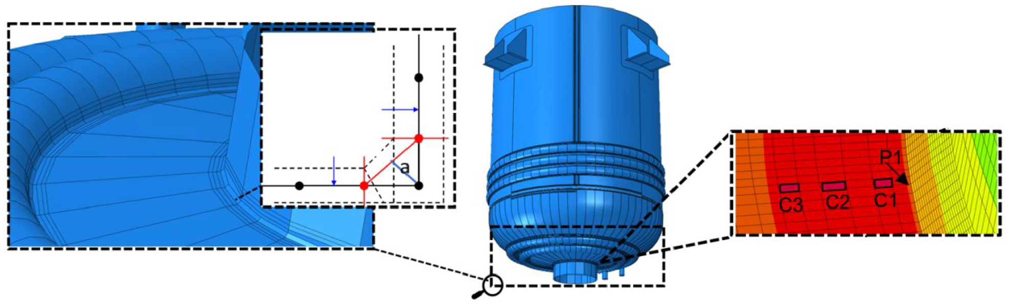
In this phase, the involvement of experts and their feedback are of paramount importance. This guides us towards monitoring critical areas, which have the highest probability of failure. At the top of the list are notably the welded areas, especially the weld at the bottom tapping point for this series of PV, which is the subject of this study (see Figure 3(a)).

(a) Identification of the maximum allowable defect by ultrasonics within the critical zone and localization of the monitoring point (P1), as well as the thickness measurement locations (P1, P2), (b) Gauge placement method according to the recommendations of the IIW to monitor point P1, as a function of the thickness “e” of the welded component on which the gauges are placed, and (c) Critical zone instrumentation.
The bottom weld, which connects the bottom tapping point to the vessel, is inspected by ultrasonography using the multi-encoding ultrasonic inspection method, according to NF EN ISO 9712, 26 NF EN ISO 13588, 27 and NF EN ISO 19285 28 standards. When the largest acceptable defect is detected, a chain consisting of three unidirectional strain gauges perpendicular to the weld is placed beyond the toe of the weld following the recommendations of the International Institute of Welding (IIW). 29 Figure 3 depicts the placement of strain gauges at point P1 where the largest defect in this weld is detected, along with an ultrasonic inspection mapping.
It should be noted that strains measured using the IIW approach, as well as the FE model detailed in the next section, do not consider defects present in the weld or residual stresses. Since service life curves were obtained by performing fatigue tests on welded structures, they are already a function of stress level on welded components, and they implicitly incorporate the effect of residual stresses and defects present in the weld.
The three strain gauges in each set, named C1, C2, and C3, are placed at distances respectively 0.4 times the support thickness, 0.9 times the support thickness, and 1.4 times the support thickness (in mm) from the weld toe. Quadratic extrapolation is then applied to provide information on the stress at the weld toe, as proposed by CODAP 30 and IIW 29 :

where
To determine whether the strain and therefore stress state at the welds is uniaxial or multiaxial, a unidirectional strain gauge perpendicular to the first gauge C1 and thus parallel to the weld is positioned. This gauge is denoted as J1.
Another important aspect of this study concerns the thickness variation at the bottom part of the equipment, which is formed by stamping. Incorrect estimation of this variation can lead to errors in estimating the stress level at the weld connecting the hemi-sphere to the branch. To address this, ultrasonic thickness measurements were conducted at points P1 (the thinnest) and P2 (the thickest) located at the top of the hemi-sphere. These measurements allow for adjustments to the FE model. The probe used during these experimental works is of type 5L16. Table 2 summarizes the results obtained for the thickness measurements.
Thickness measurement around the monitoring point.
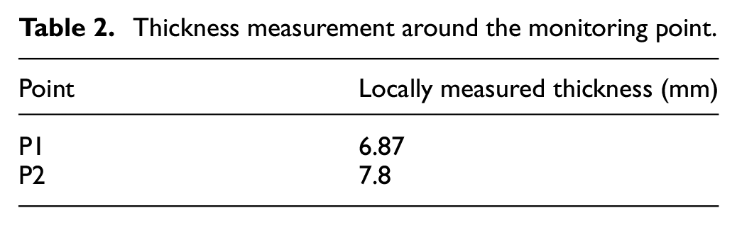
Following these results, it is noteworthy that the thickness at the hemi-sphere exhibits a substantial variation, ranging from 7.8 mm at point P2 to 6.87 mm at point P1. Thus, this thickness variation will be considered in the FE model through a linear thickness degradation function between the two ends of the hemi-sphere. To validate the FE model at the critical zone, static deformation measurements are recorded.
Experimental results and analysis
A constant pressure of 5.3 bar in the shell and 3.8 bar in the coils are applied. Figure 4 depicts the deformation levels recorded on each gauge at point P1.

Experimentally measured level of deformation at the gauges perpendicular to the welds, at 5.3 bar in the shell.
Following the experimental results, it can be observed that the deformation level at the critical zone reaches a maximum value of 307.04 μm/m perpendicular to the weld, then gradually decreases away from the weld to reach 208.4 μm/m at gauge C3. In the circumferential direction, gauge J1 records 342.5 μm/m. By analyzing the ratio between these two deformation levels, which reaches 0.89, it is evident that the stress state is biaxial at this critical point. The accuracy of our FE model, and thus that of our DT, will be linked to the accuracy of modeling and predicting the fatigue life in this area of the PV.
This section has provided us with an insight into the deformation level in the critical zone of the PV (P1), with high risk of damage. Subsequently, these results will be used to validate the FE model in this critical zone (P1).
Numerical model
The objective of this section is to detail the numerical model of the DT. This component represents the classical approach for fatigue damage calculation. Although stress levels can be determined using analytical formulas found in codes such as CODAP, 30 the development of an FE model, validated by experimental data, is preferred for a more reliable and accurate prediction of behavior.
Finite element model
Modelling and boundary conditions
To represent the behavior of the PV, it is imperative to understand its mode of operation and proceed with a meticulous numerical reproduction of the conditions to which it is exposed. The robust anchoring of the equipment to its support through the four supports, securely fastened by screws to prevent any displacement or sliding of the PV, induces fixed boundary conditions. These conditions restrict displacements and rotations in all directions at the bracket level. Furthermore, the equipment is suspended, meaning that the force of gravity affects the entire system. As for the upper and lower flanges, their design aims to minimize bending when exposed to the internal pressure of the PV. This design results in a single resultant force directed normal to the flange in the z direction (vertical axis). Subsequently, the flanges are modeled by forces referred to as bottom effects, which express the influence of pressure on the flange surfaces. These forces thus globally represent the impact of the flange on the entire PV.
Figure 5 illustrates the boundary conditions applied to the numerical model.

Boundary conditions applied to the PV.
Based on the experimental results, the thickness of the lower part of the PV varies. This variation is caused by the stamping process. Consequently, this degradation in thickness is modeled by a linear thickness degradation function applied along the half-sphere between these two ends as shown in Figure 6.

Thickness degradation function.
Weld modelling and mesh adjustment
To perform a damage calculation and considering the use of the quadratic extrapolation method as proposed by IIW, 29 precise modeling of the welds and mesh adaptation are necessary. Due to the relatively small thickness of the plates and the absence of thermal cycling, there is no high stress gradient in the thickness. In this situation, according to CODAP, 30 the PV is modeled using shell elements (S4R according to Abaqus nomenclature, a 4-node, quadrilateral, stress/displacement shell element with reduced integration and a large-strain formulation).
According to the IIW recommendations, solutions are adopted for modeling fillet welds when using shell elements. This choice is also motivated by our aim to ensure the reactivity of the FE model with reduced computational time. As per Handtschoewercker, 31 for penetrating fillet welds, it is recommended to place nodes directly at the toe of the weld bead and then connect them with an additional element having a thickness equivalent to that of the weld throat, to model the weld’s stiffness. Additionally, mesh adjustment for quadratic extrapolation is necessary, which involves placing nodes at 0.4 times the thickness, 0.9 times the thickness, and 1.4 times the thickness from the toe of the weld bead. Furthermore, to ensure mesh convergence, the methodology prescribes an element length not more than 0.4 times the thickness at the hot spot.
It is important to note that, since the weld is fully penetrating, there is no risk of crack initiation at the root. Therefore, it is assumed unnecessary to consider the nominal throat stress.
Figure 7 depicts the adapted and meshed structure.
PV with adapted mesh for quadratic extrapolation and damage calculation.
Numerical results and model validation
Figure 8 shows the simulation results with a pressure of 5.3 bar in the shell, and 3.8 bar in the coils.

Maximum principal stress field (MPa) obtained from the FE model.
The model comprises 602,494 elements. The results obtained from the FE model reveal that the critical zone is located at the bottom nozzle, with a maximum principal stress level of 108.8 MPa. Comparing these results with experimental data confirms the validity of the most critical zone.
To validate the FE model in the critical zone at point “P1,” the strain levels are compared under the application of 5.3 bar in the shell and 3.8 bar in the coils. Table 3 shows the comparison between the different results. It is noted that for the welded zones, C1, C2, and C3 represent the three strain gauges placed perpendicular to the weld for quadratic extrapolation. J1 represents the gauge perpendicular to C1 and therefore parallel to the weld.
Comparison of numerical and experimental strain results for welded areas

For a multiaxial stress state, the transformation of strains into stresses relies on the generalized Hooke’s law (equations (2) and (3)). In a complementary validation approach, special attention is given to the measured strains at gauges C1 and J1, located closest to the toe of the weld. Subsequently, a reevaluation of the discrepancy between the numerical and experimental stresses is undertaken, thus reinforcing the robustness of the analysis (see Table 4).


where
Comparison of numerical and experimental stress results for welded areas (MPa).

At the critical zone, the errors between the numerical and experimental models are acceptable, less than 11%, ensuring the accuracy of the FE model, and thus the accuracy of the DT that will be applied to this area of the PV.
Damage post-processing
Given the large size of the critical zone, consisting in 19,050 elements, the use of traditional incremental calculations for fatigue post-processing becomes prohibitively time-consuming. This approach would be too costly and impractical for our situation. It means that we cannot fully exploit the concept of the DT in its ideal reactive form. Consequently, considering our constraints in terms of computation time and the need to comply to the approach proposed by PV construction codes, we have opted for the use of S/N curve-based approaches for our fatigue damage calculation.
The objective of this section is to perform a numerical comparison among several fatigue criteria. This study will be conducted at the critical zone at the nozzle, the area with the highest level of deformation, which will determine the equipment’s life.
Reference S/N curves
In accordance with the standards outlined in section C11.3 of the CODAP, the S/N curves utilized is probabilistic representations of double-slope Basquin curves given by equation (4), with a 2.28% probability of failure. The selection of this type of double-slope curve is motivated by the consideration of loading variability. Thus, cycles with small stress ranges are not neglected by the model. These curves incorporate specific parameters such as the type and quality of the weld, as well as residual stresses and other factors related to the welding process.

where
The curves used in the CODAP standards tend to be overly conservative as they are primarily used for design purposes. In our context, focused on PV monitoring, we aim for a more realistic approach by positioning at a 50% probability of failure. Indeed, the distribution of the logarithm of cycle numbers follows a normal distribution for a given stress level in the limited endurance domain. To increase the probability of failure to 50%, equation (5) is used:

where
Table 5 provides the various parameters used for fitting the Basquin S/N curves depicted in Figure 9, with a 2.28% and 50% probability of failure. The stress ratio used for the S/N curve of the welded zone is R = 0.1.
Basquin double slope curve parameters, with FAT the weld class (characteristic fatigue strength of the weld detail in MPa at 2 million cycles),


Double slope Basquin curve.
Stress state analysis
The fatigue criterion and the equivalent stress used for damage calculation, following the quadratic extrapolation of the stress tensor, significantly influences the results. Indeed, the complexity of the local stress state determines the most appropriate fatigue criterion. In our case study, the rate of biaxiality of the stress state (a) detailed in equation (6) plays an important role. It is represented by the ratio between the principal stresses
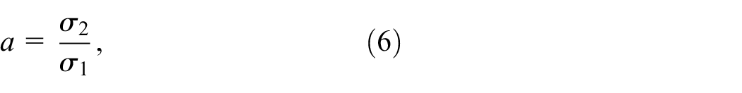

At the critical point P1, the biaxiality rate remains nearly constant across the entire loading spectrum (as shown in Figure 2), with a value of 0.8, as shown in Figure 10. Additionally, the angle (

Biaxiality rate at critical point P1.
Fatigue criteria
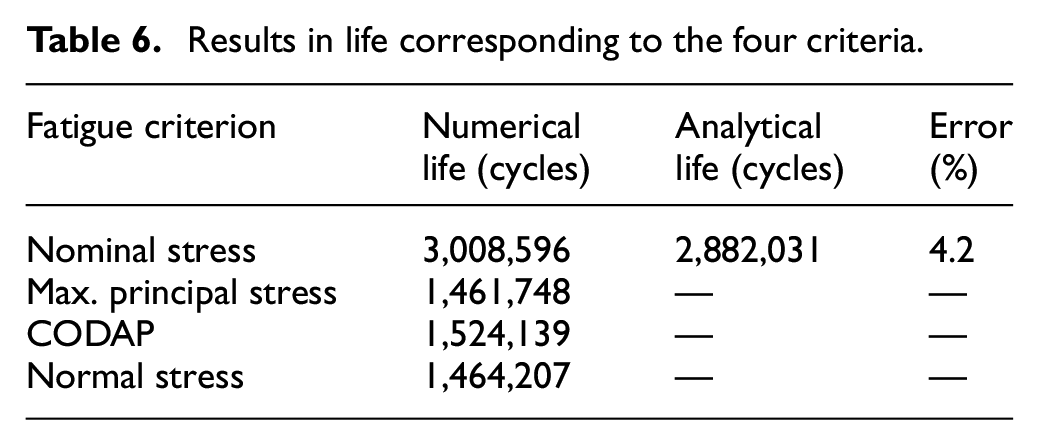
A comparative analysis among different criteria identified in the literature has been conducted. This comparison focuses on the uniaxial criterion, which relies on the use of the maximum principal stress, and simple multiaxial critical plane criteria. The results of this comparison, expressed in terms of fatigue life, are then presented in Table 6.
Results in life corresponding to the four criteria.
CODAP approach
The criterion proposed by the CODAP is a multiaxial critical plane type criterion. This approach explores all potential planes within a 360° sphere around the critical point to find the critical plane where maximum damage occurs. The equivalent stress considered, detailed in equations (8)–(10), maximizes the shear stress range between two instances on the plane in question. The stress
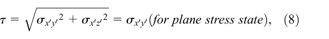


with

CODAP – figure C11.3.9.2.3a – definition of the analysis plane using the reference plan Ox′y′z′ and the angles θ and φ: (1) analysis plan, (2) initial plan, and (3) normal to the analysis.
Normal stress approach
The critical plane method discussed in this paragraph analyzes the stress state along various planes normal to the surface of the component. By considering the normal stress on each plane (equation (11)) and evaluating the damage using the Basquin curve, the critical plane where maximum damage occurs is identified. Unlike the CODAP approach, this method proposes an angular discretization of 10°, allowing calculations to be performed on 18 material planes.

With
Result and discussion
The critical zone is primarily influenced by the pressure in the shell, a comparative study is conducted to select the best approach. This involves fatigue post-processing of stress results from a loading cycle in the shell with an amplitude of 5.3 bar, which locally translates, at the point P1, to a maximum principal stress amplitude of 108.6 MPa. Table 6 offers an overview of the PV life evaluated using the four criteria.
Preliminary comparison between the two life estimations based on numerical and experimental data from the gauges (see Table 4) was conducted. In this step, the estimation is performed using a uniaxial approach focusing on the stress perpendicular to the weld. We observe that a 3.4% error in stress results in a 4.2% error in life, which is deemed acceptable for a high life fatigue calculation. However, when comparing the numerical results obtained with a uniaxial and multiaxial approaches, we notice that the latter are quite similar (between 1,461,748 and 1,524,139 cycles), and markedly different from the uniaxial approach, with almost a factor of 2 difference between the two. This disparity can be explained by the simple proportional multiaxial stress state present at the critical zone. The uniaxial method underestimates the effective maximum stress on the critical plane because it does not account for all stress components and their variation in the critical plane orientation. To illustrate the influence of the difference between stress levels obtained using the “nominal stress” and “normal stress” approaches on the fatigue life, we refer to the mathematical interpretation of the S/N equation. The critical plane approach, which considers the maximum normal stress, shows that damage reaches its peak on the critical plane oriented at 90°. In this case, the normal stress reaches 106.18 MPa, which is nearly 20 MPa higher than the simplified uniaxial approach based on nominal stress, which yields 86.63 MPa. These results are consistent with those presented in Table 4, where the longitudinal stress (
Referring to the S/N equation, this stress difference has an exponential impact on fatigue life. Equation (12) illustrates this influence,

where
Thus, an increase of 20 MPa in the stress level leads to a reduction of approximately 50% in fatigue life. This explains the difference of a factor of 2 between the multiaxial approaches, which have almost identical stress levels, and the uniaxial approach.
Multiaxial criteria prove to be the most suitable and accurate for estimating service life. It is worth noting that, given the similarity of multiaxial approaches, it is possible to opt for using the maximum principal stress instead of approaches based on critical plane searching, for a quicker, simplified, and efficient analysis.
Digital twin in service
Figure 12 depicts the architecture of the DT employed for monitoring the mechanical fatigue of the PV. The setup of this DT requires an offline phase involving several steps such as the development and adjustment of the FE model, as well as the selection of the appropriate fatigue model.

Digital twin concept.
The first step involves creating an FE model representative of the real system to predict stress and strain fields on the PV based on variations in service pressures. This model is then validated by comparing its mechanical behavior with that of the actual PV. Abaqus software, Smith, 32 is used for simulation. Once the numerical model is validated, it allows us to access information on stress throughout the critical area, including point P1.
The second step entails selecting the most appropriate damage model to predict the PV’s accumulated damage and remaining life. Considering computational time constraints and compliance with PV construction codes, CODAP, and welding institute recommendations, IIW, for addressing fatigue issues in welded areas, an S/N curve-based approach is favored. This approach estimates the PV’s remaining life based on the applied stress level, relying on reference curves established by relevant standards and codes. HBM-nCode software, nCode, 33 is used.
Once operational, and the models are selected, the pressure data is transmitted to an acquisition system and stored in the cloud via IoT. This data can be retrieved at regular intervals from the cloud using automation scripts by the DT for post-processing, enabling real-time estimation of fatigue damage and remaining service life in the critical zone.
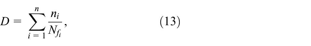
The DT can monitor fatigue damage in the PV under constant nominal load. Additionally, it can detect damage caused by unexpected variations in cyclic loading, such as pressure spikes during startup, disruptions in pump operation, or deliberate decisions to increase pressure. These variations can accelerate the damage process by transitioning from one load block to another with higher amplitude. Indeed, the entire local stress spectrum is subjected to the Rainflow cycle counting method, Matsuiski and Endo, 34 at each time interval. This algorithm discretizes the stress history into a defined number “n” of amplitude classes, facilitating better management of these situations. Subsequently, the linear damage accumulation law of Miner, detailed in equation (13), is utilized to assess the progressive damage rate of the equipment:
where
Figure 13 depicts the information flow in the fatigue post-processing process used by the DT to quantify damage.

Data flow on fatigue post-processing.
Table 7 presents the evolution of damage in the critical zone at the nozzle (point P1), at different time steps.
Damage monitoring in critical zone.

The calculated lifecycle in Paragraph 3.2.4 represents the approach used during the design phase for a constant pressure loading (5.3 bar in the tank in our case) over the PV’s life. According to the results, using the maximum principal stress for a cycle with an amplitude of 108.6 MPa and a period of 7 s, the lifecycle is estimated at 1,461,748 cycles, corresponding to approximately 4 months of continuous cycling. Therefore, the estimated damage for 1 month of continuous cycling according to equation (13) is D = 0.25. However, as observed in Table 7, the real-time damage displayed by the DT after 1 month of loading is 0.15, equating to 219,262 cycles instead of the 365,437 cycles anticipated during the design phase. This discrepancy is explained, as illustrated in Figure 14, by considering the PV downtime (effective loading time) as well as the variation in pressure amplitude.

(a) Real time pressure effective loading and (b) cycle counting of pressure specter with Rainflow method.
On the left of Figure 14, the graph shows the operating pressure applied in the equipment as a function of time, while on the right, a cycle count links the amplitude of each pressure cycle to the number of corresponding cycles and their average pressure. A high cycle density can be observed at low pressure amplitudes. However, their effect on damage remains negligible due to their low amplitude, less than the cut-off limit.
However, many cycles have amplitudes between 2 and 6.3 bar. It is important to note that any pressure amplitude more than 2 bar contributes to ESP damage. Theoretically, cycling was planned at 5.3 bar, but the operating procedure revealed the occurrence of additional cycles beyond this amplitude during the 4 months of operation. These unplanned cycles also contributed to ESP damage, in particular the loading peaks that occurred after cycling stops and restarts. These life-damaging peaks, acknowledged by the operators, are clearly visible after the second shutdown and restart, when a maximum pressure of 9.5 bar was reached. This corresponds to a maximum local principal stress of 191 MPa, exerting a critical effect on the equipment’s fatigue strength.
Conclusion
In this work, a Digital Twin (DT) has been developed to monitor the progressive fatigue damage of a Pressure Vessel (PV) and offer predictive maintenance. Firstly, a critical zone inspection was conducted to ensure the absence of defects not compliant with the standard code. This inspection enabled us to identify the most critical point (P1) at the tapping, where strain gauges were installed. Subsequently, a Finite Element (FE) model faithful to the behavior of the physical twin was developed and validated using experimental data from the in-situ gauges. Once the numerical model is validated, it has allowed us to access information on damage throughout the critical area, including point P1. Following this, several fatigue criteria were tested. The conclusions drawn from the results indicate that the multiaxial criteria have shown superior performance compared to uniaxial ones in our case study. The results reveal that the stress state along the loading spectrum is multiaxial proportional, with invariance in the direction of the principal axes. Thus, the choice was made for multiaxial approaches, using the maximum principal stress as the equivalent stress. Finally, the proposed DT has been developed and used to estimate the progressive fatigue damage of the equipment. It can regularly monitor the evolution of loading in real-time and update itself with data from the physical model in service.
The DT can monitor the damage rate of the equipment under constant nominal loads as well as under random loads and can also consider the impact of sudden pressure surges. Additionally, it can monitor inaccessible critical areas on the PV, making it easier to make decisions about future inspections. In the same way, it enables the simulation of planned solicitation scenarios before their implementation to predict the effect of these planned load spectra on the equipment’s life.
Despite all the capabilities of this DT, it has some limitations. While it provides surveillance of the structure’s integrity, this approach may be limited to a specific configuration or situation, and therefore less suited to unforeseen circumstances. For example, if major modifications occur, such as significant deformations, corrosion, or the emergence of a defect, the initial FE model is unable to consider them, as it is specific to a given case study. Thus, this methodology could be limited in terms of considering the variety of possible scenarios affecting a structure in service. Following this study, it is imperative to broaden the concept of the DT so that it can ensure the surveillance of the structure’s integrity while adapting to the multitude of scenarios the structure in service could encounter, and speeding up the computation from near real-time calculation (a few minutes of computation) to real-time (a few seconds of computation). However, several challenges remain. One major issue lies in the instrumentation of equipment: determining the optimal number of sensors to use and strategically placing them to ensure effective monitoring while minimizing costs. Future work will address these limitations and questions, including subjecting the PV to failure to verify the DT predictions by comparing them with experimental results.
Footnotes
Handling Editor: Yuansheng Zhou
Ethical considerations
This article does not contain any studies with human or animal participants. There are no human participants in this article and informed consent is not required.
Author contributions
The report was written by Izat Khaled, who served as the corresponding author. Modesar Shakoor and Dmytro Vasiukov reviewed the results and revised the article. Mohamed Bennebach and Salim Chaki also contributed by revising the report and leading the project.
Funding
The author(s) disclosed receipt of the following financial support for the research, authorship, and/or publication of this article: We would like to acknowledge: The French Association Nationale de la Recherche et de la Technologie (ANRT) and the French Centre Technique des Industries Mécaniques (CETIM) for the funding of the PhD work used in this publication, as well as the French Région Hauts-de-France and Institut Mines-Télécom IMT Nord Europe for the contribution to the funding of JUNAP project.
Declaration of conflicting interest
The author(s) declared the following potential conflicts of interest with respect to the research, authorship, and/or publication of this article: Bennebach Mohamed reports financial support was provided by Technical Centre for the Mechanical Industries, and financial support was provided by National Association of Technical Research. The authors declared no potential conflicts of interest with respect to the research, authorship, and/or publication of this article.