Sage Journals: Discover world-class research

Abstract

This paper introduces the development of a self-propelled hard hose traveler to accelerate the transition of the traditional JP50-180 hard hose traveler toward becoming an irrigation robot and enhancing its applicability in farmland. The uniformity model of linear motion water distribution is established by utilizing the total frequency of application during the sprinkler motion and the radial application depth once during the fixed sprinkler rotation. The average application depth deviation between the tested and calculated values is 7.4%. The effect of combined irrigation with sprinkler motion is superior to that of motion irrigation with a single sprinkler. The average application depth decreases as the motion speed increases while the water distribution uniformity (CU value) remains constant. The average application depth decreases as the path spacing increases. In contrast, the CU value first increases and then decreases. The highest CU value is approximately 94%, with the optimal path spacing being 1.5R and the optimal combinations of sprinkler rotation angles α, β, and γ being 0°, 90°, and 90°, or 90°, 90°, and, 0°, or 0°, 180°, and 0°, respectively depending on the case. The above indicators are significant for planning the irrigation application of a self-propelled hard hose traveler.

Keywords

Uniformity of water distribution average application depth sprinkler motion speed calculation model path spacing sprinkler rotation angle

Introduction

With the intensifying issues of global population aging and shortage of agricultural labor, agricultural robots are entering a period of rapid development.¹ Extensive research has already been conducted in various fields, including agriculture,^2–5 orchards,^6–9 protected agriculture,^10–13 and livestock and poultry farming.^14,15 Water-saving irrigation equipment also evolves toward intelligence and autonomous mobility.¹⁶ The traditional hard hose traveler is continuous-moving water-saving irrigation equipment driven by a water turbine, suitable for medium-sized farmland in the plains of China.^17,18 However, its applicability still needs improvement. Therefore, this paper designs a self-propelled hard hose traveler using an electric tracked vehicle to carry the sprinkler and drag out the polyethylene tube, achieving continuous irrigation. This design addresses irrigation issues in sloping fields and fields with poor regularity through its off-road climbing and maneuvering capabilities. Furthermore, the design also provides the necessary hardware foundation for water-saving irrigation equipment to evolve into sprinkler irrigation robots.

The hydraulic parameters, such as the sprinkler motion speed, the path spacing, and the flow rate, are crucial factors influencing the application depth of the sprinkler irrigation system.^19,20 The average application depth is somewhat equivalent to the irrigation quota in the irrigation schedule. This irrigation quota determines whether the field moisture meets the crop water requirements.^21,22 Therefore, this paper designs the hydraulic parameters for the self-propelled hard hose traveler using traditional hard hose traveler and irrigation scheduling.

Apart from the application depth, the CU value is also a critical indicator²³ for evaluating the hydraulic performance of motion sprinkler irrigation²⁴ and combined sprinkler irrigation.²⁵ Experiments may encounter irregular factors due to the influence of operating conditions,²⁶ as well as natural environmental factors^27,28 (such as temperature and humidity). Researchers have explored the relationship between operating conditions, the CU value, and the average application depth by establishing calculation models in such cases. The existing calculation models simplify radial water distribution lines into regular shapes, such as triangles or ellipses,²⁹ using time as the dependent variable. Then, this formula is integrated to calculate the CU value. However, simplifying radial lines results in poor accuracy.³⁰ Ge et al.¹⁷ represented the radial water distribution lines using cubic spline interpolation, Lagrange interpolation, and polynomial fitting. The author compared these simplification methods. The CU values were calculated and validated using the same calculation model. The results indicate that the cubic spline curve and polynomial fitting methods were the best, with a maximum deviation of less than 10%. Therefore, this paper represents the radial water distribution lines based on the cubic spline interpolation curve and derives the total application depth at each measurement point through the calculation model. Compared to previous studies,^17,29,30 the calculation model established in this paper determines the total application depth at each measurement point based on the total application frequency during the sprinkler motion and the radial application depth once during the fixed sprinkler rotation. This model refines the motion process of each irrigation event and sprinkler rotation, aiding in the comprehensive analysis throughout the paper of the influence of various hydraulic parameters, such as sprinkler arrangement, sprinkler rotation angle, and path spacing, on hydraulic performance.

The traditional hard hose traveler primarily relies on a single sprinkler layout, with an average CU value of only 62% for a single sprinkler in operation, indicating poor performance.^31,32 Ge et al.³³ conducted research on combined irrigation with this sprinkler motion. The author analyzed multiple sprinkler rotation angles and path spacings through a calculation model using the 50PYC vertical oscillating sprinkler gun. The CU value first increased and then decreased as the path spacing increased. Moreover, the sprinkler rotation angle also significantly impacted the CU value. The results showed that the optimal range for the sprinkler rotation angle is 240°–320°, while the optimal range for the path spacing is 1.5R–1.7R, with a CU value higher than 85%. When Hills et al.³⁴ operated the lateral-move sprinkler system at speeds ranging from 10% to 100% of its maximum motion speed, the CU value ranged between 92% and 96%. Furthermore, as the motion speed increased, the CU value decreased slightly. In addition, a close correlation was observed between the average application depth and the motion speed. Li et al.³⁵ found that the CU value of center-pivot sprinkler systems decreases slightly as the motion speed increases. The above literature demonstrates that sprinkler rotation angle, path spacing, and sprinkler motion speed impact the CU value of the self-propelled hard hose traveler. Since the sprinkler adopts a double-sprinkler arrangement and sprays water toward both sides of the path with a sprinkler rotation angle of less than or equal to 180°, this paper will consider the abovementioned factors.

In summary, this paper first designs the hydraulic parameters for the hard hose traveler. Subsequently, a calculation model for the irrigation performance of the sprinkler in straight-line movement is established and experimentally validated. The impact of various factors on the average application depth and CU value is explored to derive the optimal hydraulic parameters and the effective operating area per hour, laying the foundation for the promotion and application of the sprinkler.

Self-propelled hard hose traveler and hydraulic parameters

Composition and working principle of sprinkler

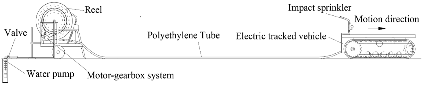
The self-propelled hard hose traveler is designed based on the traditional hard hose traveler, which can be remotely controlled. Its structure mainly comprises a reel truck, polyethylene tube, electric tracked vehicle, sprinkler, and motor-gearbox system, as shown in Figure 1. The reel truck is designed with the maximum recommended flow rate. The electric tracked vehicle mainly comprises a crawler, frame, servomotor, driver, 4G antenna, storage battery, controller, and reduction gearbox, adopting a double-sprinkler arrangement, as shown in Figure 2.

Figure 1.

Components and working modes of the self-propelled hard hose traveler.

Figure 2.

Electric tracked vehicle and sprinkler arrangement.

The reel truck has the functions of unfolding, storing, and retracting the polyethylene tube. The electric tracked vehicle is characterized by its maneuverability and flexible walking. The vehicle loads sprinklers, mainly changing the irrigation position, unfolding polyethylene tube, and guiding. The motor-gearbox system provides power for retracting the polyethylene tube and replacing the water turbine of the traditional hard hose traveler. During sprinkling irrigation, the reel truck is stored at the water source. The electric-tracked vehicle moves away from the hose reel cart, pulls out the polyethylene tube, and achieves mobile sprinkling irrigation. The polyethylene tube is disconnected from the electric-tracked vehicle at the end of the sprinkling irrigation operation. The motor-gearbox system drives the reel to rotate and retract the polyethylene tube. Then, the electric-tracked vehicle is transferred to the next sprinkling point.

Hydraulic parameters and influencing factors

The irrigation quota is affected by factors such as crops, regions, seasonal irrigation quotas, and irrigation frequency. The average sprinkler application depth should be higher than the irrigation quota. This paper designs the hydraulic parameters of the self-propelled hard hose traveler based on the structure of the traditional hard hose traveler of JP50-180 type produced by Jiangsu Huayuan Water-saving Co., Ltd. Hydraulic parameters mainly include the flow range of the sprinkler, the deployment speed and length of polyethylene tube, and the average application depth. The corresponding values of the traditional hard hose traveler of JP50-180 type are 5.5–19.7 m³ h⁻¹, 6–30 m h⁻¹, 180 m, and 6–44 mm, respectively. Therefore, the average application depth of the self-propelled hard hose traveler is set as 6–44 mm to meet the irrigation quota.

The application depth and CU value are related to the sprinkler flow rate, layout, type, rotation angle, motion speed, path spacing, and nozzle size. The remaining factors remain unchanged to adjust the application depth of the sprinkler. The sprinkler motion speed is estimated via the average application depth. The traditional hard hose traveler is equipped with a single 40PY₂ impact sprinkler and a maximum flow rate of 19.7 m³ h⁻¹. Therefore, the flow rate of the single sprinkler of the self-propelled hard hose traveler is 9.85 m³ h⁻¹. A 30PY₂ impact sprinkler with a nozzle diameter of 10.5 × 4.5 mm is selected from the national standard for rotating sprinklers GB/T 22999-2008.³⁶ Its working pressure is approximately 450 kPa, an elevation angle of 25°, and a range of 25 m.

During the sprinkler’s movement, if the measuring points are still within the circle with the sprinkler as the center and the range as the radius, it is called unfinished watering (except for the measuring points that have not been watered). Otherwise, it is called finished watering.

In Figure 3, the points represent impact sprinklers, and A, B, and C are three irrigated areas. An impact sprinkler moves along the motion path while rotating and spraying at a 180° angle. The ratio of travel distance to spray radius during the rotation cycle of the impact sprinkler is relatively small; therefore, the impact sprinkler can be considered stationary. When the sprinkler is at point 2, the range can radiate to points 1 and 3. When the sprinkler head is at point 3, the range can radiate to points 2 and 4. The application depth from point 1 to point 2 in area B is the same as from point 2 to point 3 in area A. The application depth from the sprinkler at point 2 to point 3 in area C is the same as that from point 3 to point 4 in area B. Theoretically, the application depth from the sprinkler at point 1 to point 2 is in area A, and each measuring point is fully watered. Therefore, the relationship between the average application depth and the motion speed of the sprinkler can be obtained, as shown in equation (1).

H_{1} = \frac{10^{9} \times Q t_{1}}{n_{1} \times 10^{3} \times R \times 10^{3} \times S} = \frac{10^{3} Q}{n_{1} Rv}

v = \frac{10^{3} Q}{n_{1} R H_{1}}

(1)

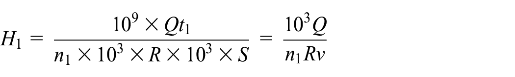
where H₁ is the average application depth when designing hydraulic parameters, mm; v is the motion speed of the sprinkler, m h⁻¹; R is the impact sprinkler range, m; Q is the maximum flow rate of the reel truck, m³ h⁻¹; n₁ is the number of sprinklers; S is the motion distance of the sprinkler, m; t₁ is the motion time of the sprinkler, h.

Figure 3.

Partially irrigated areas in sprinkler irrigation.

An inverse proportional function with a coefficient of 398.4 can be obtained based on the above calculations; the fitting coefficient of the function is 1. The sprinkler motion speed is temporarily set at 10–50 m h⁻¹, with an accuracy of 1 m h⁻¹. This paper takes the path spacing, sprinkler rotation angle, and sprinkler motion speed as influencing factors to investigate the average application depth and CU value, as shown in equations (2) and (3). Table 1 shows the values of various factors in this paper.

h = f (L_{C}, α, β, γ, v)

(2)

CU = g (L_{C}, α, β, γ, v)

(3)

where h is the application depth at a measuring point, mm; L_C is the path spacing, m; α, β, and γ are combined as the sprinkler rotation angles, and the sum of the three is 180°, °; the CU value is the uniformity of water distribution, %.

Table 1.

Values of influencing factors.

Serial number	Influencing factor		Values
1	Sprinkler motion speed (m h⁻¹)		10, 15, 20, 25, 30, 35, 40, 45, 50
2	Sprinkler rotation angles (°)	α	0, 15, 30, 45, 60, 75, 90
		β	90, 105, 120, 135, 150, 165, 180
		γ	0, 15, 30, 45, 60, 75, 90
3	Multiple of path spacing		1.0, 1.1, 1.2, 1.3, 1.4, 1.5, 1.6, 1.7, 1.8, 1.9, 2.0

Uniformity model of linear motion water distribution

A radial water distribution curve based on the cubic spline polynomial

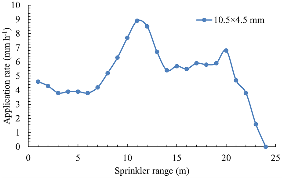
The superposition method of calculating the water volume of the motion sprinkler is based on the radial water distribution of the fixed sprinkling irrigation of the 30PY₂ impact sprinkler in the laboratory. Under the same flow, the impact sprinkler with 180° rotation for 0.5 h receives the water the same number of times as 360° rotation for 1 h. The water distribution of the nozzle with a diameter of 10.5 × 4.5 mm is shown in Figure 4. According to the verification method of the radial water volume line,^36,37 the deviation between the test value and the calculated average application rate is within 4%. The cubic spline function interpolation method is used to calculate the radial water distribution of the sprinkler based on previous research.³⁸ The water distribution line is shown in equation (4). The rotation period of the fixed sprinkler T (s) was recorded when the sprinkler rotated at 180°. The application frequency K of the fixed sprinkling irrigation is shown in equation (5):

ρ (z) = {\begin{matrix} A_{1} z^{3} + B_{1} z^{2} + C_{1} z + D_{1}, (z_{0} < z < z_{1}) \\ A_{2} z^{3} + B_{2} z^{2} + C_{2} z + D_{1}, (z_{1} < z < z_{2}) \\ ⋮ \\ A_{i} z^{3} + B_{i} z^{2} + C_{i} z + D_{i}, (z_{i - 1} < z < z_{i}) \end{matrix}

(4)

K = INT (\frac{1800}{T}) + 1

(5)

where z is the distance from the sprinkler to the measuring point, m; ρ(z) is the application rate based on the distance between the sprinkler and the measuring point, mm h⁻¹; A_i, B_i, C_i, and D_i are the coefficients of equation (4); z_i is polynomial nodes with integer values, m.

Figure 4.

Water distribution of 30PY₂ impact sprinkler.

The method of motion water volume superposition

The method of motion water volume superposition calculates the total application depth at each measuring point by utilizing the total frequency of application during the sprinkler motion and the radial application depth once during the fixed sprinkler rotation. Figure 5 shows the water condition of an M point during the sprinkler motion. Figure 5(a) shows the change process in the nozzle rotation direction. Figure 5(b) shows the relationship between the sprinkler and the position changes of measurement point M. Figure 5(c) shows the relationship between the position of measurement point M, the sprinkler motion, and the rotation angle of the sprinkler. The sprinkler positions are represented as M_start and M_end, for point M starting and ending the water-receiving process, respectively; the distance between these two positions is L (m). The angles between the sprinkler and the upper and lower sides of the motion path are α and γ, respectively, while the rotation angle of the sprinkler is β. The sum of α, β, and γ angles is 180°.

Figure 5.

The water condition of an M point during the sprinkler motion: (a) The change process in the nozzle rotation direction, (b) The relationship between the sprinkler and the position changes of measurement point M, (c) The relationship between the position of measurement point M, the sprinkler motion, and the rotation angle of the sprinkler.

The dynamic process of the sprinkler includes uniform motion along the path and periodic rotation. The motion distance of the sprinkler is divided into multiple units according to the sprinkler rotation period. Two dynamic processes are independent during the calculation process. The distance between point M and the sprinkler is calculated when the sprinkler is at each unit. The result was factored into equation (4) to obtain the application depth. Once the sprinkler motion is finished, the total application depth of the M point is calculated as the sum of the water received in each unit.

Three hypotheses are proposed based on the information above:

(1) The sprinkler jet morphology and the water distribution in the range of water application are the same during each rotation period.

(2) The change in distance between the point measured and the sprinkler should be ignored during each rotation period.

(3) The influence of wind speed, direction, temperature, and humidity on water distribution under natural conditions should be neglected.

The projection distance l (m) between the sprinkler position and the measuring point on the motion path can be determined once the M point is watered, as shown in equation (6):

l = {\begin{matrix} \sqrt{R^{2} - x_{m}^{2}}, x_{m} \geq R \sin γ \\ x_{m} \cot γ, x_{m} < R \sin γ \end{matrix}

(6)

where x_m is the distance from measuring point M to the motion path, m.

Next, the rotation period t₂ (s) of the motion sprinkler and the radial motion distance Δl (m) within the period are determined, as shown in equations (7) and (8), respectively:

t_{2} = \frac{β}{180^{°}} T

(7)

Δ l = \frac{v t_{2}}{3600}

(8)

Then, the radial motion length L of the sprinkler is determined. Assuming that the measuring point M moves radially while the sprinkler sprays in a fan-shaped area with an angle of β, point M is only watered within the fan-shaped area. Therefore, within the fan-shaped boundary, the length of the line passing through point M and parallel to the motion path is the motion length L of the sprinkler, as shown in Figure 5(c) and equation (9):

L = {\begin{matrix} \sqrt{R^{2} - x_{m}^{2}} + x_{m} \cot γ, R \sin α < x_{m} < R \sin γ \\ \sqrt{R^{2} - x_{m}^{2}} + x_{m} \cot α, R \sin γ < x_{m} < R \sin α \\ 2 \sqrt{R^{2} - x_{m}^{2}}, x_{m} \geq R \sin α, and, x_{m} \geq R \sin γ \\ x_{m} (\cot α + \cot γ), x_{m} < R \sin α, and, x_{m} < R \sin γ \end{matrix}

(9)

Next, the positional relationship between the sprinkler and measuring point M is determined. Parameter L is divided into n units, as shown in equation (10). Each unit is labeled as Δl with j∈ (0, n), and equation (11) is derived to calculate the distance ΔL (m) from the starting point M_start to the unit j. The distance d_j (m) from unit j to point M is shown in equation (12):

n = INT (\frac{L}{Δ l}) + 1

(10)

Δ L = j Δ l

(11)

d_{j} = \sqrt{{| l - Δ L |}^{2} + x_{m}^{2}} = \sqrt{{| x_{m}^{2} \cot^{2} γ - j Δ l |}^{2} + x_{m}^{2}}

(12)

Next, the application depth h (d_j) (mm) of point M in a single rotation period of the sprinkler and the application depth h_n (mm) in the n periods of rotation are calculated using equations (13) and (14), respectively:

h (d_{j}) = \frac{ρ (d_{j})}{K} = \frac{ρ (d_{j})}{INT (\frac{1800}{T}) + 1}

(13)

h_{n} = \sum_{j = 0}^{n} h (d_{j}) = \sum_{j = 0}^{n} \frac{ρ (d_{j})}{INT (\frac{1800}{T}) + 1}

(14)

The average application depth and the uniformity of water distribution

According to the national standards GB/T 27612.3-2011³⁹ and GB/T 21400.1-2008,⁴⁰ the measuring points should be arranged in a radial or grid pattern. The average application depth H is shown in equation (15). The uniformity of water distribution can be calculated through the above model,⁴¹ as shown in equation (16):

H = \frac{1}{N} \sum_{m_{1} = 1}^{N} h_{n} = \frac{1}{N} \sum_{m_{1} = 1}^{N} \sum_{j = 0}^{n} \frac{ρ (d_{j})}{INT (\frac{1800}{T}) + 1}

(15)

CU = (1 - \frac{\sum_{m_{1} = 1}^{N} | h_{n} - H |}{\sum_{m_{1} = 1}^{N} h_{n}}) \times 100

(16)

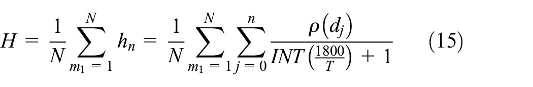
where H is the average application depth, mm; m₁ is the serial number of the measurement point; and N is the total number of measurement points.

Validating the average application depth

In this study, the straight-line motion of the sprinklers and a single row of the measuring points completely exposed to water were adopted to validate the accuracy of the application depth of the calculated and test values. The test was conducted in the Lizhong Agricultural Machinery Cooperative in Huantai, Zibo City, Shandong Province, China. The radial line of the measuring point is perpendicular to the motion path, and the buckets are arranged in a 1.5 × 1.5 m form, as shown in Figure 6. The sprinkler was accelerated to the required speed and moved through mechanical dragging. The average value of application depth was recorded after completing the test, obtaining a lateral line of the measuring point completely exposed to water. A JP50-180 hard hose traveler, a 30PY₂ impact sprinkler, and a 10.5 × 4.5 mm nozzle diameter were selected in the test. The sprinkler moves at a speed of 35 m h⁻¹ with a flow rate of 9.96 m³ h⁻¹, α = 0°, β = 180°, and γ = 0°. The installation height of the sprinkler is 1.3 m. The caliber of the plastic bucket was 200 mm, and the height was 170 mm. The wind speed ranged from 1.23 to 2.55 m s⁻¹. The relative temperature of air was maintained at 12.3°C, and the relative humidity of air was maintained at 24.82%. The test values are compared with the calculated values as follows.

Figure 6.

Bucket layout and sprinkler irrigation test site diagram.

Figure 7 shows the curves of calculated and test values of application depth for the motion sprinkler, with average application depths of 10.46 and 11.28 mm, respectively. The deviation rate between the two values is 7.4%. The test value is higher than the calculated value. The minimum deviation occurs at 10.5 m, with a deviation rate of 0%. In comparison, the maximum deviation occurs at 15 m, with a deviation rate of 20.9%. The overall trend of the test application depth curve can support the trend of the calculated value curve, indicating that the calculated value is accurate. Nevertheless, some deviations were present. The accuracy may be caused by mode and test calculations, the evaporative drift of water, and the deviation rate during the sprinkling process. Overall, the test value can validate the accuracy and reliability of the calculation method.

Figure 7.

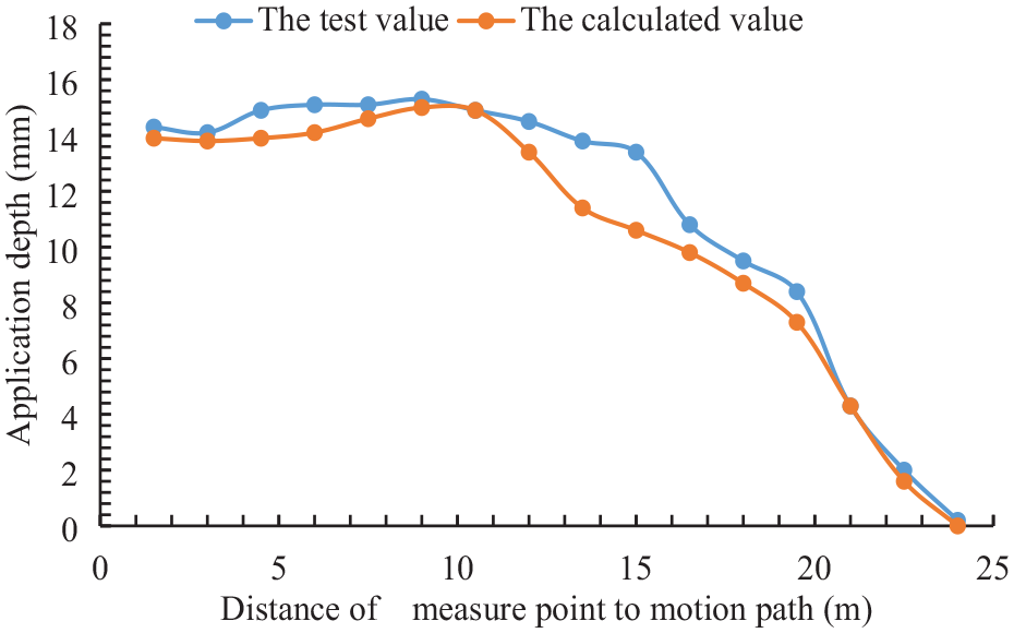
Application depth curves of the calculated and test values.

Irrigation performance of the sprinkler in straight-line movement

Motion irrigation with a single sprinkler

Sprinkler motion speed

As illustrated in Table 2, when the sprinkler rotation angles are set to α = 0°, β = 180°, and γ = 0°, the average application depth decreases in a power function form as the motion speed increases, as indicated by equation (17). The fitting coefficient for this relationship is 1. Figure 8 presents the application depth at each measurement point for various speeds. At different speeds, the application depth at each measurement point also varies in a power function form:

H = 366.29 v^{- 1.001}

(17)

Table 2.

The average application depth and CU values at various motion speeds.

Motion speed (m h⁻¹)	The average application depth (mm)	The CU value (%)
10	36.6	62.80
15	24.4	62.83
20	18.3	62.92
25	14.6	62.78
30	12.2	62.76
35	10.5	62.90
40	9.2	62.84
45	8.1	62.72
50	7.3	62.98

Figure 8.

Average application depth for sprinklers at various motion speeds.

In Table 2, the CU value exhibits slight oscillatory changes as the motion speed increases but generally remains within the 62.7%–63.0% range. The fluctuation range of the CU value at 0.3% is relatively narrow and insufficient to demonstrate the impact of motion speed on water distribution. Additionally, fluctuations in the CU value may also be caused by variations in Δl and the value taken after the decimal point. Therefore, the impact of sprinkler motion speed on the CU value can be neglected.

Sprinkler rotation angle

The application depths at various measurement points for different sprinkler rotation angles and the sprinkler motion speed of 35 m h⁻¹ are shown in Figure 9. The average application depths and CU values are presented in Table 3. In Table 3, the combinations of α, β, and γ angles have been numbered, and the application depth generally remains within the range of 10.4–11.0 mm. Relative deviations in the average application depth can be observed due to value selection and model calculation deviations.

Figure 9.

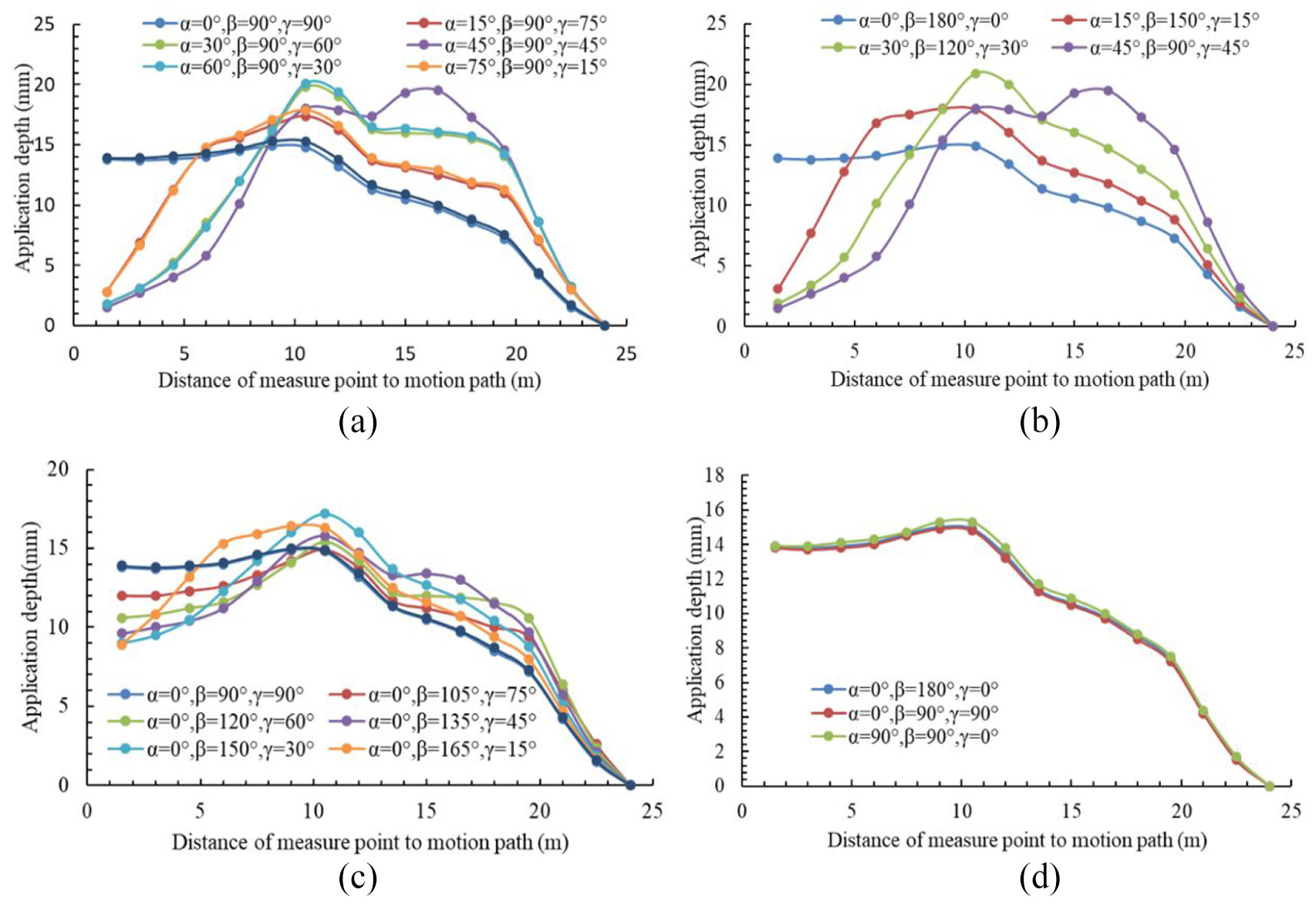
The application depth lines for different sprinkler rotation angles: (a) β angle remains at 90°, (b) the centerline of β angle is perpendicular to the motion path, (c) α angle is constantly at 0° while β angle gradually increases, and (d) comparison of β angle at 90° with that at 180° for α or γ either being 0°.

Table 3.

The average application depth and CU value for different sprinkler rotation angles.

Number	α (°)	β (°)	γ (°)	Average application depth (mm)	CU value (%)	Corresponding to the image
1	0	90	90	10.4	62.56	Figure 9(a)
2	15	90	75	10.8	60.21
3	30	90	60	10.9	47.24
4	45	90	45	11.0	40.96
5	60	90	30	11.0	46.38
6	75	90	15	11.0	59.84
7	90	90	0	10.6	63.05
8	0	180	0	10.5	62.90	Figure 9(b) with the addition of data for number 4.
9	15	150	15	10.9	54.98
10	30	120	30	10.9	46.82
11	0	105	75	10.4	71.09	Figure 9(c) with the addition of data for numbers 1 and 8.
12	0	120	60	10.5	72.99
13	0	135	45	10.5	68.98
14	0	150	30	10.6	65.29
15	0	165	15	10.6	63.47

In Figure 9(a), when β is 90°, each application depth lines for each α angle ranging from 0° to 90° largely coincide with those for γ angles ranging from 0° to 90°, with similar CU values. When α or γ angle is 90°, the application depth line remains flat until it reaches 10 m, after which it starts to decline. When either α or γ angle is 90°, the application depth volume line remains straight and exhibits a downward trend at 10 m. The values at both ends of other application depth volume lines are relatively low, while those in the middle are high.

Different sprinkler rotation angles are compared next. When α increases from 0° to 45°, the application depth is lower at the 1–9 m range and higher at the 10–24 m range. Conversely, the opposite pattern is observed when α decreases from 45° to 0°. In Table 3, as α increases, the CU value first decreases and then increases, with the lowest and highest values being approximately 40.96% and 63%, respectively.

In Figure 9(b), angles α and γ are the same, and β is higher than or equal to 90°. As either angle α or γ increases, the starting value of the application depth line decreases. In contrast, the intermediate values increase, causing the irrigation water to accumulate toward the rear. In Table 3, as angle α or γ increases, the CU value decreases, with the lowest and highest values being 40.96% and 62.90%, respectively.

In Figure 9(c), α = 0°, β ≥ 90°, and γ ≤ 90°. The application depth lines at β = 90° and 180° are taken as references. The higher the β angle within the range of 90°–135°, the lower the starting value of the application depth line, and the more pronounced the trend of being lower on both sides and higher in the middle. The higher the β angle within the range of 135°–180°, the higher the starting value of the application depth line, and the more pronounced the trend of smoothly decreasing. In Table 3, the CU value is highest at β = 120°, with a value of 72.99%. When β = 90° or 180°, the CU value is lowest, with a value below 63%.

In Figure 9(d), the application depth lines for the three sprinkler rotation angles almost coincide, and the CU values in Table 3 are approximately the same. The highest CU value (73.0%) is achieved when α is 0°, β is 120°, and γ is 60°. Therefore, the following discussion will focus on the application depth and CU value by adjusting the two path spacing.

Combined irrigation with sprinkler motion

When arranged at a path spacing of 2.0 R, the sprinkling effect of the sprinklers is identical to the effect when they are not combined. Therefore, further discussion on this aspect is omitted below.

Sprinkler motion speed

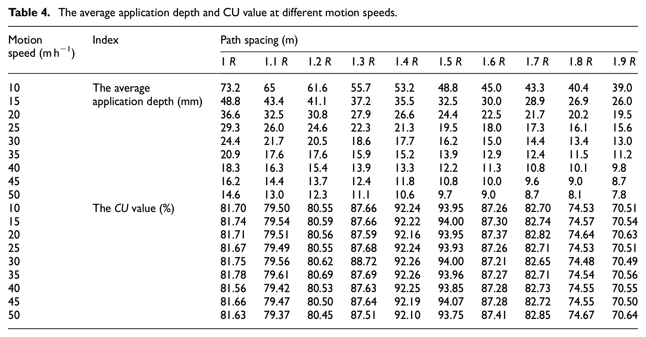
Table 4 shows the average application depth and CU values for different motion speeds, with α at 0°, β at 180°, and γ at 0°. For the same path spacing, the average application depth decreases continuously as the motion speed increases while the CU value remains constant. As the path spacing increases, the average application depth decreases continuously for the same motion speed. In contrast, the CU value increases and decreases. The optimal path spacing in this paper is 1.5 R, with the CU value maintained at approximately 94%. The relationship between the motion speed and the average application depth is shown in equation (18):

H = 491.56 v^{- 1.003}

(18)

Table 4.

The average application depth and CU value at different motion speeds.

Motion speed (m h⁻¹)	Index	Path spacing (m)
Motion speed (m h⁻¹)	Index	1 R	1.1 R	1.2 R	1.3 R	1.4 R	1.5 R	1.6 R	1.7 R	1.8 R	1.9 R
10	The average application depth (mm)	73.2	65	61.6	55.7	53.2	48.8	45.0	43.3	40.4	39.0
15		48.8	43.4	41.1	37.2	35.5	32.5	30.0	28.9	26.9	26.0
20		36.6	32.5	30.8	27.9	26.6	24.4	22.5	21.7	20.2	19.5
25		29.3	26.0	24.6	22.3	21.3	19.5	18.0	17.3	16.1	15.6
30		24.4	21.7	20.5	18.6	17.7	16.2	15.0	14.4	13.4	13.0
35		20.9	17.6	17.6	15.9	15.2	13.9	12.9	12.4	11.5	11.2
40		18.3	16.3	15.4	13.9	13.3	12.2	11.3	10.8	10.1	9.8
45		16.2	14.4	13.7	12.4	11.8	10.8	10.0	9.6	9.0	8.7
50		14.6	13.0	12.3	11.1	10.6	9.7	9.0	8.7	8.1	7.8
10	The CU value (%)	81.70	79.50	80.55	87.66	92.24	93.95	87.26	82.70	74.53	70.51
15		81.74	79.54	80.59	87.66	92.22	94.00	87.30	82.74	74.57	70.54
20		81.71	79.51	80.56	87.59	92.16	93.95	87.37	82.82	74.64	70.63
25		81.67	79.49	80.55	87.68	92.24	93.93	87.26	82.71	74.53	70.51
30		81.75	79.56	80.62	88.72	92.26	94.00	87.21	82.65	74.48	70.49
35		81.78	79.61	80.69	87.69	92.26	93.96	87.27	82.71	74.54	70.56
40		81.56	79.42	80.53	87.63	92.25	93.85	87.28	82.73	74.55	70.55
45		81.66	79.47	80.50	87.64	92.19	94.07	87.28	82.72	74.55	70.50
50		81.63	79.37	80.45	87.51	92.10	93.75	87.41	82.85	74.67	70.64

Sprinkler rotation angle

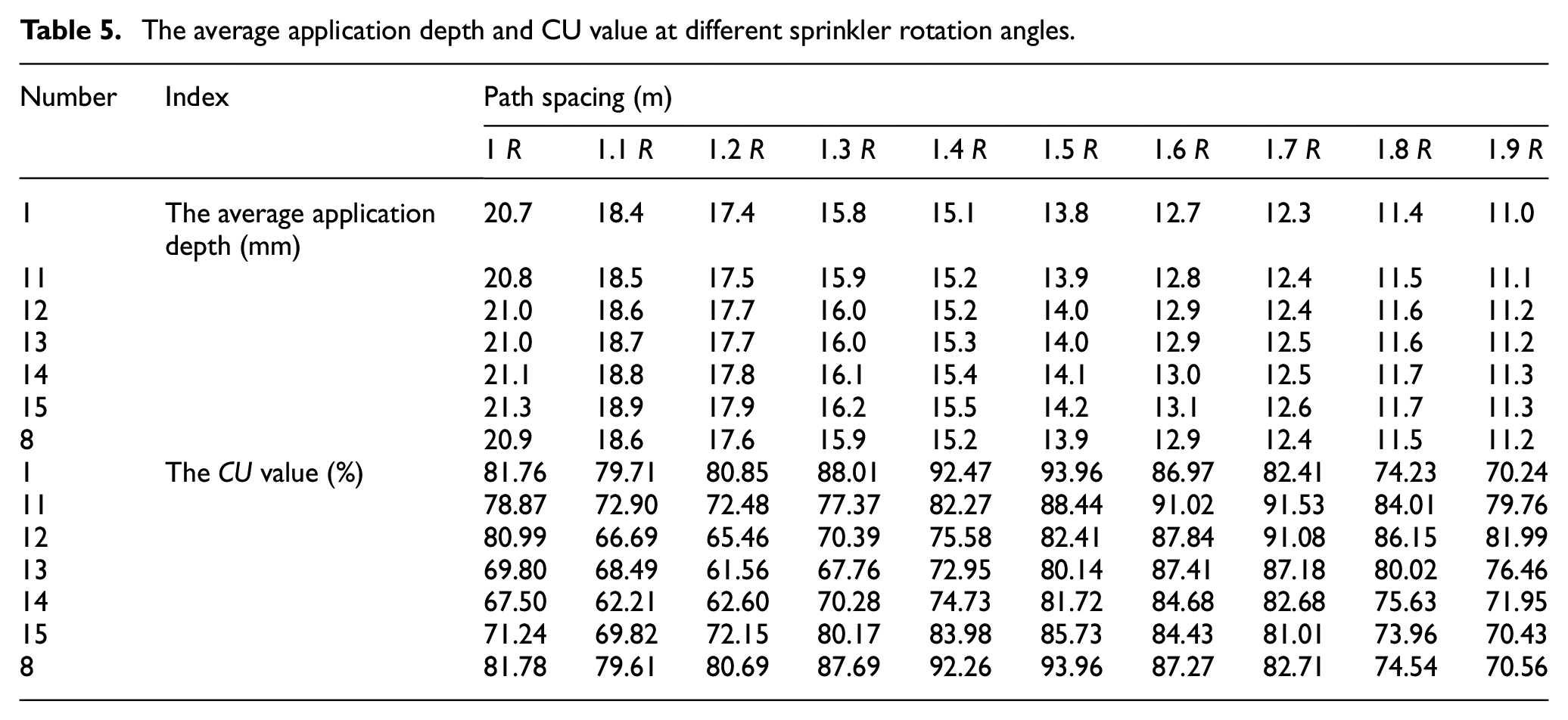
Table 5 shows the average application depth and CU values for different sprinkler rotation angles, with the sprinkler motion speed at 35 m h⁻¹. Different sprinkler rotation angles are marked in Table 3. At the same path spacing, the deviation range of the average application depth is within 0.6 mm. The CU value first decreases and then increases. The average application depth gradually decreases with an increase in path spacing. The basic trend of the CU value is to increase first and then decrease. The average application depth and CU value for numbers 1 and 8 are almost identical. In this paper, the highest CU value is approximately 94%, with the optimal combined spacing being 1.5 R. The optimal angles for α, β, and γ are either 0°, 90°, and 90°, 90°, 90°, and 0°, or 0°, 180°, and 0°.

Table 5.

The average application depth and CU value at different sprinkler rotation angles.

Number	Index	Path spacing (m)
Number	Index	1 R	1.1 R	1.2 R	1.3 R	1.4 R	1.5 R	1.6 R	1.7 R	1.8 R	1.9 R
1	The average application depth (mm)	20.7	18.4	17.4	15.8	15.1	13.8	12.7	12.3	11.4	11.0
11		20.8	18.5	17.5	15.9	15.2	13.9	12.8	12.4	11.5	11.1
12		21.0	18.6	17.7	16.0	15.2	14.0	12.9	12.4	11.6	11.2
13		21.0	18.7	17.7	16.0	15.3	14.0	12.9	12.5	11.6	11.2
14		21.1	18.8	17.8	16.1	15.4	14.1	13.0	12.5	11.7	11.3
15		21.3	18.9	17.9	16.2	15.5	14.2	13.1	12.6	11.7	11.3
8		20.9	18.6	17.6	15.9	15.2	13.9	12.9	12.4	11.5	11.2
1	The CU value (%)	81.76	79.71	80.85	88.01	92.47	93.96	86.97	82.41	74.23	70.24
11		78.87	72.90	72.48	77.37	82.27	88.44	91.02	91.53	84.01	79.76
12		80.99	66.69	65.46	70.39	75.58	82.41	87.84	91.08	86.15	81.99
13		69.80	68.49	61.56	67.76	72.95	80.14	87.41	87.18	80.02	76.46
14		67.50	62.21	62.60	70.28	74.73	81.72	84.68	82.68	75.63	71.95
15		71.24	69.82	72.15	80.17	83.98	85.73	84.43	81.01	73.96	70.43
8		81.78	79.61	80.69	87.69	92.26	93.96	87.27	82.71	74.54	70.56

Results and discussion

Hydraulic parameter matching and performance analysis

The optimal CU values for motion irrigation with a single sprinkler and combined irrigation with sprinkler motion are approximately 70% and 94%, respectively. Figure 10 demonstrates the irrigation effect with a sprinkler motion speed of 35 m h⁻¹ and the sprinkler rotation angles α, β, and γ of 0°, 180°, and 0°, respectively. Additionally, Figure 11 shows the irrigation effect with a sprinkler motion speed of 35 m h⁻¹ and a path spacing of 1.5 R. At the same motion speed, the application depth pattern in Figure 11 is significantly better than that in Figure 10. Combined irrigation with sprinkler motion can be applied to elongated field plots, whereas motion irrigation with a single sprinkle suits irregularly shaped field plots. If the average application depth exceeds the scope of this study, its value can be calculated using equations (17) and (18). Therefore, the highest CU value obtained in this paper is approximately 94%, with the optimal combined spacing being 1.5 R. The optimal angles for α, β, and γ are the following combinations: 0°, 90°, and 90°; 90°, 90°, and 0°; 0°, 180°, and 0°, respectively.

Figure 10.

The irrigation effect with a sprinkler motion speed of 35 m h^−1.

Figure 11.

The irrigation effect with a sprinkler motion speed of 35 m h⁻¹ and a path spacing of 1.5 R.

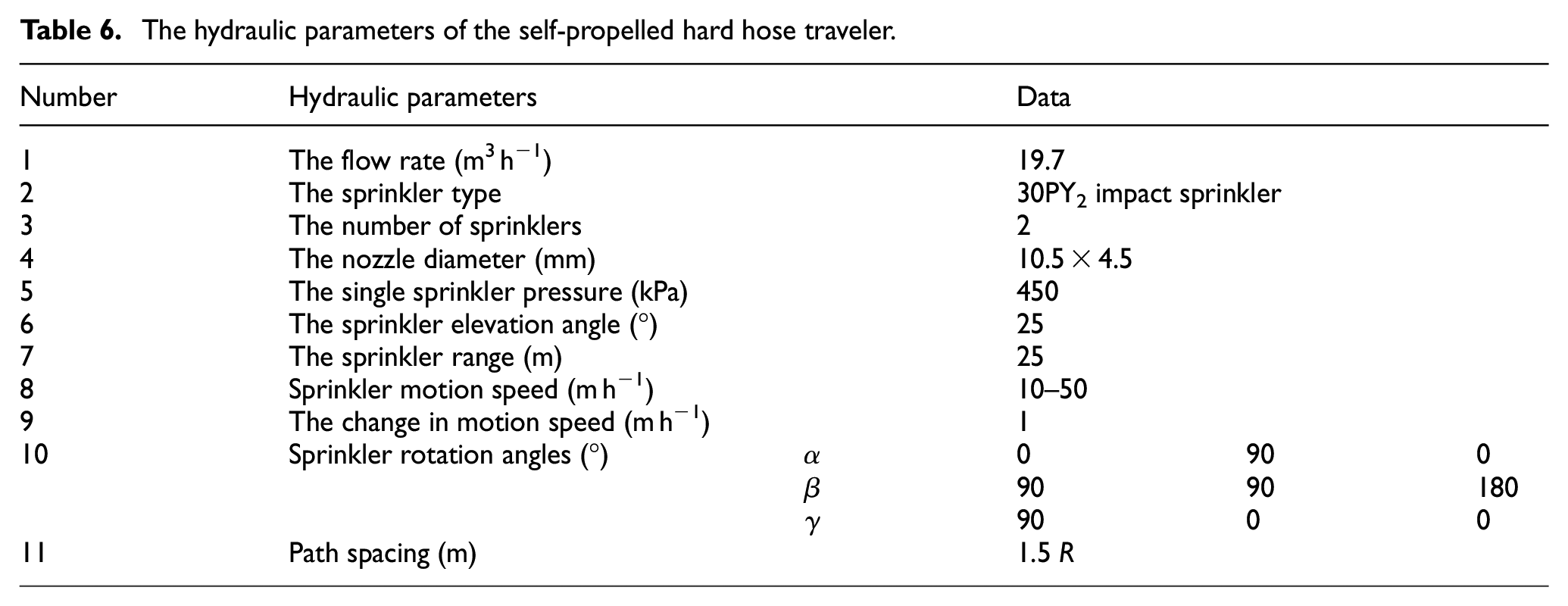
The hydraulic parameters of the self-propelled hard hose traveler are listed in Table 6. These parameters serve as important guidelines for field sprinkler irrigation operations.

Table 6.

The hydraulic parameters of the self-propelled hard hose traveler.

Number	Hydraulic parameters		Data
1	The flow rate (m³ h⁻¹)		19.7
2	The sprinkler type		30PY₂ impact sprinkler
3	The number of sprinklers		2
4	The nozzle diameter (mm)		10.5 × 4.5
5	The single sprinkler pressure (kPa)		450
6	The sprinkler elevation angle (°)		25
7	The sprinkler range (m)		25
8	Sprinkler motion speed (m h⁻¹)		10–50
9	The change in motion speed (m h⁻¹)		1
10	Sprinkler rotation angles (°)	α	0	90	0
		β	90	90	180
		γ	90	0	0
11	Path spacing (m)		1.5 R

Effective operating area per hour

In addition to the average application depth and CU value, this paper also sets the effective operating area per hour D (m² h⁻¹) as an evaluation index, specifically as shown in equation (19). The effective operating area per hour refers to the area that can be irrigated per hour by a self-propelled hard hose traveler during a single deployment of the polyethylene tube at the optimal path spacing. The deployment operation time refers to the duration for a self-propelled hard hose traveler to fully deploy the polyethylene tube in a single continuous movement at a specific speed. The above indicators are characterized by high guiding significance for planning the irrigation application of self-propelled hard-hose travelers. The detailed data is shown in Table 7.

D = L_{C} v

(19)

Table 7.

The effective operating area per hour of a self-propelled hard hose traveler.

Sprinkler motion speed (m h⁻¹)	One deployment operation time (h)	Effective operating area per hour (m² h⁻¹)
10	18.00	360.0
15	12.00	540.0
20	9.00	720.0
25	7.20	900.0
30	6.00	1080.0
35	5.14	1260.7
40	4.50	1440.0
45	4.00	1620.0
50	3.60	1800.0

Conclusions

The JP50-180 self-propelled hard hose traveler employs a double-sprinkler arrangement for linear irrigation operations, utilizing 30PY₂ impact sprinklers with a nozzle diameter of 10.5 × 4.5 mm. The uniformity of water distribution was analyzed by combining computational modeling and test validation, leading to the determination of optimal hydraulic parameters. These findings have laid a solid foundation for promoting and applying this sprinkler. The specific conclusions of this paper are as follows:

(1) A self-propelled hard hose traveler was designed to elucidate the design principle for the sprinkler motion speed range from 10 to 50 m h⁻¹. A calculation model for the uniformity of linear motion water distribution was established. Test validation showed that the average application depth deviation between the test and calculated values was 7.4%. A power equation relationship was presented between the sprinkler motion speed and the average application depth rate.

(2) The average application depth decreases with increased motion speed during motion irrigation with a single sprinkler. At the same time, the CU value remains approximately constant. The average application depth for different sprinkler rotation angles stays within the range of 10.4–11.0 mm. The CU value is optimal when α is 0°, with a value of roughly 70%.

(3) The average application depth decreases as the motion speed increases during the combined irrigation with sprinkler motion and under the same path spacing. In contrast, The CU value remains approximately constant. As the path spacing increases, the average application depth decreases at the same motion speed, and the CU value first increases and then decreases. The effect of combined irrigation with sprinkler motion is superior to that of motion irrigation with a single sprinkler. In this paper, the highest CU value is approximately 94%, with the optimal path spacing being 1.5R and the optimal sprinkler rotation angles α, β, and γ being one of the following combinations: 0°, 90°, and 90°; 90°, 90°, and 0°; or 0°, 180°, and 0°. The effective operating area per hour is provided for each motion speed.

Currently, this paper only studies the irrigation performance of the double-sprinkler arrangement for self-propelled hose reel sprinklers, without exploring various types of sprinkler arrangements. In the future, comprehensive performance research on this sprinkler system will be conducted, incorporating aspects such as irrigation performance, energy consumption, and operational capabilities, to facilitate its gradual maturity.

Footnotes

Acknowledgements

We would like to thank MogoEdit () for its English editing during the preparation of this manuscript.

Handling Editor: Sharmili Pandian

Declaration of conflicting interests

The author(s) declared no potential conflicts of interest with respect to the research, authorship, and/or publication of this article.

Funding

The author(s) disclosed receipt of the following financial support for the research, authorship, and/or publication of this article: This research was supported by the following grants: Natural Science Foundation of the Jiangsu Higher Education Institutions of China (24KJB210020); the Key Laboratory of Fluid and Power Machinery (Xihua University), Ministry of Education (LTDL-2024015); Suzhou Vocational University (202305000003, KY202304003).

ORCID iDs

Zhengdian Xu

Daoxing Ye

References

Liu

Gong

Yuan

, et al. Current status and development trends of agricultural robots. Trans Chin Soc Agric Mach 2022; 53: 1–22+55. (in Chinese)

Mccool

Beattie

Firn

, et al. Efficacy of mechanical weeding tools: a study into alternative weed management strategies enabled robotics. IEEE Robot Autom Lett 2018; 3: 1184–1190.

Bao

Gai

Xiang

, et al. Field robotic systems for high-throughput plant phenotyping: a review and a case study. In: Zhou

Nguyen

(eds) High-throughput crop phenotyping. Concepts and strategies in plant sciences. Cham: Springer, 2021, pp.13–38.

Zhou

Luo

, et al. Design and test of laser-controlled paddy field levelling-beater. Int J Agric Biol Eng 2020; 13: 57–65.

Zhai

Zheng

, et al. Establishment and experimental verification of deep learning model for on-line recognition of field cabbage. Trans Chin Soc Agric Mach 2022; 53: 293–303. (in Chinese)

Fang

Zhao

, et al. Fruit yield prediction and estimation in orchards: a state-of-the-art comprehensive review for both direct and indirect methods. Comput Electron Agric 2022; 195: 106812.

Majeed

Karkee

Zhang

, et al. Development and performance evaluation of a machine vision system and an integrated prototype for automated green shoot thinning in vineyards. J Field Robot 2021; 38: 898–916.

Granland

Newbury

Chen

, et al. Detecting occluded y-shaped fruit tree segments using automated iterative training with minimal labeling effort. Comput Electron Agric 2022; 194: 106747.

Zhou

Zhang

, et al. Design, development, and field evaluation of a rubber tapping robot. J Field Robot 2022; 39: 28–54.

10.

Atefi

Pitla

, et al. In vivo human-like robotic phenotyping of leaf traits in maize and sorghum in greenhouse. Comput Electron Agric 2019; 163: 104854.

11.

Lee

Kam

Min

, et al. A vision servo system for automated harvest of sweet pepper in Korean greenhouse environment. Appl Sci 2019; 9: 2395.

12.

Gong

Wang

, et al. Robotic harvesting of the occluded fruits with a precise shape and position reconstruction approach. J Field Robot 2022; 39: 69–84.

13.

Huang

Choi

, et al. Picking dynamic for robotic harvesting of Agaricus bisporus mushrooms. Comput Electron Agric 2021; 185: 106145.

14.

Vroegindeweij

Vanhell

Igsselmuiden

, et al. Object discrimination in poultry housing using spectral reflectivity. Biosyst Eng 2018; 167: 99–113.

15.

Feng

Wang

Design of disinfection robot for livestock breeding. Procedia Comput Sci 2020; 166: 310–314.

16.

Zhu

Zhao

Yuan

, et al. Current situation and development considerations of mechanized irrigation in hilly and mountainous areas. J Drain Irrig Mach Eng 2024; 42: 294–303. (in Chinese)

17.

Zhu

DL.

Application of different curve interpolation and fitting methods in water distribution calculation of mobile sprinkler machine. Biosyst Eng 2018; 174: 316–328.

18.

Liu

Zhu

Yuan

, et al. Research and development trend of agricultural water-saving sprinkler and micro-irrigation equipment in China. J Drain Irrig Mach Eng 2022; 40: 87–96. (in Chinese)

19.

Wan

Zhu

Tian

, et al. Translocating speed ration effect on water distribution uniformity of lightweight lateral move irrigation system. Water Sav Irrig 2016; 9: 87–89+93. (in Chinese)

20.

Tian

Zhu

Wan

, et al. Development and performance test of lateral move irrigation system. J Drain Irrig Mach Eng 2017; 35: 357–361.

21.

Guo

YY.

Farmland water conservancy. Beijing: China Water & Power Press, 2007.

22.

Ali

(ed.). Crop water requirement and irrigation scheduling. In: Fundamentals of irrigation and on-farm water management. Vol. 1. New York, NY: Springer Science & Business Media, 2010, pp.399–451.

23.

Burt

Clemmens

Strelkoff

, et al. Irrigation performance measures: efficiency and uniformity. J Irrig Drain Eng 1997; 123: 423–442.

24.

Khalid

Abdalhaleem

ElKamil

, et al. Impacts of center pivot irrigation system uniformity on growth of potato crop and residual soil nitrogen. Int J Agric Biol Eng 2019; 12: 126–131.

25.

Shi

Zhu

, et al. Effect of different working conditions on water for sprinkler irrigation. J Drain Irrig Mach Eng 2021; 39: 318–324.

26.

Xiang

Qureshi

Tunio

, et al. Low-pressure drop size distribution characterization of impact sprinkler jet nozzles with and without aeration. Agric Water Manag 2021; 243: 106458.

27.

Emanuele

Bernardo

Lessandro

, et al. Wind drift and evaporation losses of a mechanical lateral-move irrigation system: oscillating plate versus fixed spray plate sprinklers. Agric Water Manag 2019; 225: 105759.

28.

Hussein

Mohamed

Ahmed

, et al. Prediction of wind drift and evaporation losses from sprinkler irrigation using neural network and multiple regression techniques. Agric Water Manag 2018; 195: 211–221.

29.

DF.

The design and calculation of resultant uniformity of continuously moving mechanical sprinkler systems. J North China Inst Water Conservancy Hydroelectr Power 1984; 6: 40–52. (in Chinese)

30.

Bittinger

Longenbaugh

RA.

Theoretical distribution of water from a moving irrigation sprinkler. Trans ASAE 1962; 5: 26–30.

31.

Smith

Baillie

Gordon

. Performance of travelling gun irrigation machines. In: Proceedings of the conference of the Australian society of sugar cane technologists (ed Hogarth

D M

), Cairns, QLD, Australia, 29 April–2 May 2002, pp.235–240. Brisbane: PK Editorial Services Pty Ltd.

32.

Wigginton

Raine

SR.

Irrigation water use efficiency in the Mary River catchment: on-farm performance evaluations in the dairy sector. Toowoomba, QLD: National Centre for Engineering in Agriculture Publication, 2001, pp.17–26.

33.

Zhu

DL.

Construction and application of mobile spraying uniformity model of hard hose traveler. Trans CSAE 2016; 32: 130–137. (in Chinese with English abstract)

34.

Hills

Rumsey

JW.

Lateral move water application uniformity relative to machine speed. Trans ASAE 1988; 31: 527–530.

35.

Hui

Yan

HJ.

Effects of travel speed and collector on evaluation of the water application uniformity of a center pivot irrigation system. Water 2020; 12: 1916.

36.

GB/T 22999. Rotating sprinkler. Beijing: SPC, 2009. (in Chinese)

37.

Seginer

Kantz

Nir

, et al. Indoor measurement of single-radius sprinkler patterns. Trans ASAE 1992; 35: 523–533.

38.

Molle

Gat

YL.

Model of water application under pivot sprinkler. II: calibration and results. J Irrig Drain Eng 2000; 126: 348–354.

39.

GB/T 27612.3. Agricultural irrigation equipment-sprinklers—part 3: characterization of distribution and test methods. Beijing: SPC, 2011. (in Chinese)

40.

GB/T 21400.1. Traveler irrigation machines—part 1: operational characteristics and laboratory and field test methods. Beijing: SPC, 2008. (in Chinese)

41.

Fukui

Nakanishi

Okamura

Computer evaluation of sprinkler irrigation uniformity. Irrig Sci 1980; 2: 23–32.

Uniformity of water distribution in linear movement with a double-sprinkler of self-propelled hard hose traveler

Abstract

Keywords

Introduction

Self-propelled hard hose traveler and hydraulic parameters

Composition and working principle of sprinkler

Hydraulic parameters and influencing factors

Uniformity model of linear motion water distribution

A radial water distribution curve based on the cubic spline polynomial

The method of motion water volume superposition

The average application depth and the uniformity of water distribution

Validating the average application depth

Irrigation performance of the sprinkler in straight-line movement

Motion irrigation with a single sprinkler

Sprinkler motion speed

Sprinkler rotation angle

Combined irrigation with sprinkler motion

Sprinkler motion speed

Sprinkler rotation angle

Results and discussion

Hydraulic parameter matching and performance analysis

Effective operating area per hour

Conclusions

Footnotes

Acknowledgements

Declaration of conflicting interests

Funding

ORCID iDs

References