Sage Journals: Discover world-class research

Abstract

Mechanical seals are critical components in the mechanical industry, and their operational status directly impacts the performance of pumps, compressors, and other machinery. Therefore, conducting research on the fault diagnosis of mechanical seals is essential. To enhance the accuracy of the assessment model, we propose an integrated approach that leverages the fusion of multiple graph neural networks (GNNs). Firstly, recognizing the diversity among different sensors, we utilize multi-channel data to comprehensively represent the operational state of the mechanical seal. These channels include various types of sensors such as acoustic emission and force sensors. Secondly, we employ multiple methods to transform the original multi-channel data into graph data, thereby continuously increasing the diversity of the datasets used for training. Finally, after training GNNs, we output the data of these networks through data fusion to obtain evaluation results. The effectiveness of our assessment approach is demonstrated using mechanical seal test data.

Keywords

Mechanical seal fault diagnosis graph neural networks multi-sensor data fusion

Introduction

In the era of Industry 4.0, the efficient operation and maintenance of mechanical equipment are crucial for ensuring production continuity and product quality.¹ Mechanical seals, core components in numerous rotating machines, are mechanical devices designed to prevent fluid leakage through the relative sliding of two sealing faces, maintaining the sealing effect. Their performance directly impacts the safety, reliability, and energy efficiency of equipment, being widely applied in fluid machinery operating in rotational form, such as pumps, compressors, and variable-speed gearboxes.² However, over prolonged periods of operation, mechanical seals are susceptible to various failures, such as wear and leakage, which can not only cause production disruptions but also lead to significant safety incidents and environmental issues. Consequently, research into fault diagnosis and performance assessment of mechanical seals is of paramount importance for preventive maintenance, prolonging equipment life, and safeguarding production safety.³ Traditional assessment methods for the performance of mechanical face seals predominantly rely on empirical judgment, physical experimentation, and limited sensor monitoring. These approaches are not only time-consuming and labor-intensive but also struggle to achieve satisfactory diagnostic accuracy when confronted with complex and variable operating conditions. Particularly challenging is the evaluation of end-face wear conditions under incomplete prior knowledge, often necessitating extensive sampling and cumbersome data processing. Deep learning techniques haven received more and more attention in engineering filed. For example, Yao et al.⁴ proposed a semi-supervised adversarial deep learning (SADL) method for lithium-ion battery capacity estimation, the results demonstrated that the SADL method accurately estimates the capacity of various battery types. Ma et al.⁵ proposed a multi-order graph embedding stacked denoising auto encoder optimized by an improved sine–cosine algorithm (MGE-ISCA-SDAE) and a collaborative central domain adaptation (CCDA) for rolling bearing faults diagnosis under few-shot samples. Therefore, the fault diagnostic strategy based on deep learning have received more and more attention, and a lot of fault diagnostic methods have been proposed, especially for rotation machine.⁶

GNNs are a type of deep learning model capable of processing graph-structured data. They learn node feature representations by passing information between nodes in the network, thereby enabling efficient handling of graph data.^7,8 Unlike conventional neural networks, GNNs can maintain the structural information of graphs while leveraging the relationships between nodes for feature learning.⁹ This gives them a significant edge when dealing with data characterized by intricate dependencies.¹⁰ Unlike CNNs or RNNs, GNNs directly operate on graphs where nodes represent entities and edges represent relationships.¹¹ Moreover, GNNs capture both node-level and graph-level dependencies by aggregating information from neighboring nodes. This is especially useful in tasks requiring relational information, like link prediction or node classification.¹² In the context of mechanical seal systems, the network topology formed by the deployment of sensors, along with the interactions among different physical quantities, can naturally be represented as graph data. Li et al.¹³ proposed a novel intelligent fault diagnosis and prediction framework based on GNNs, which provides three graph construction methods and studies seven graph convolutional networks with four different graph pooling methods. In order to provide benchmark results to assist further research, these models were comprehensively evaluated on eight datasets, including six fault diagnosis datasets and two prognostic datasets. This makes GNNs an ideal tool for assessing the condition of mechanical seals, as they can effectively capture and analyze the complex relationships inherent in such systems.¹⁴

The research on fault diagnosis methods for mechanical seals using GNNs with multi-sensor data fusion at the data layer is an emerging trend that leverages the complex interrelationships between sensor data to enhance diagnostic accuracy; this approach enables the direct processing of raw sensor data, capturing both spatial and temporal features through graph representations, and has shown promise in detecting and classifying various types of faults in real-world applications. The integration of multi-source data allows for a comprehensive evaluation of the seal’s condition from multiple perspectives and physical quantities, enhancing the accuracy and reliability of assessments.¹⁵ For instance, integrating various sensor data such as vibration signals,¹⁶ temperature signals, and pressure signals into a graph structure, where each sensor node not only contains its own measurement values but also connects with other nodes through edge information, forming a complex network.¹⁷ GNNs can effectively handle this kind of graph-structured data by passing and aggregating information between nodes, learning deeper feature representations, thus enabling precise assessments of the mechanical seal’s condition.

In order to assess and diagnose the running condition of mechanical seal, Fan et al.¹⁸ reviewed the condition monitoring of mechanical seals and pointed out the acoustic emission signal was suit for monitoring the running condition of seal faces. And then, Fan et al.¹⁹ proposed a MUSIC algorithm based on higher order statistics to monitoring the running condition of seal faces. Moreover, Fan et al.²⁰ modeled the acoustic emission between seal faces by using tribology method. Based on the work of Fan, Towsyfyan et al.^21,22 proposed to monitor the condition of mechanical seal based on the lubrication condition of two seal faces. However, the proposed methods only monitored the running condition of seal faces, it can not to assess the damage degree of seal faces.

We have introduced a multi-GNNs method using data layer fusion to evaluate the condition of mechanical seals in response to the above issues. The approach begins by utilizing multi-channel sensor data to capture the operational status of the mechanical seals comprehensively. This data is then transformed into graph representations using various graph construction techniques, which enriches the dataset’s diversity. After training, the assessment outcomes are derived by combining the outputs from multiple GNN models at the data layer. Experimental validation confirms that the proposed method can effectively identify different operational states of mechanical seals, such as normal operation, stationary ring (SR) damage, and rotating ring (RR) damage, while also distinguishing between varying degrees of damage. Furthermore, through comparative analysis of different model architectures and their classification accuracies, an optimal evaluation model structure is identified. In summary, the GNNs model based on data layer fusion presented here holds significant promise for enhancing the accuracy and comprehensiveness of mechanical seal condition evaluations.

Graph neural networks

GNNs^23,24 are a class of neural networks which are designed to operate on data structured as graphs. The GNNs have gained significant attention because the GNNs can effectively model relationships and dependencies in data where traditional neural networks struggle. The GNNs can implement several tasks, including node classification, graph classification, link prediction based on the relationships between nodes and topology of graph.

A graph can be represented as a set of vertices and edges, denoted as: $G = (V, E)$ , where $V = (v_{1}, v_{2}, \dots, v_{n})$ is a set with $n$ vertices and $E \subseteq V \times V$ is a set of edges. Usually, the adjacency matrix $A \in R^{n \times n}$ is used to represent the connection relationship between vertices. If each vertex contains H-dimensional features, use the feature matrix $F \in R^{n \times m}$ for representation. The principle of GNNs is that information passed the nodes, and then the nodes update. Every node of the graph would be aggregated when the information passes it from its surrounding nodes. Besides, the representation vector would be updated.

Generally, the graph should be generated firstly when training a GNNs. However, the data, which is collected from different sensors in mechanical engineering, is a one-dimension data, not a graph. Therefore, the sensor data should be converted into graph firstly. Several construction methods of graph have been researched, including:

The construction method of graph based on the Short-Time Fourier Transform (GSTFT), which is proposed by Goyal and Pabla.²⁵ The data would be divided into $N$ segments. For each segment, compute the short-time spectrum and treat the computed values as individual graph nodes:

\hat{P} (k, m) = \frac{1}{T} {| Y (k, m) |}^{2}

(1)

And then, the weight of each pair of nodes would be calculated by using the Euclidean distance.

The visibility graph²⁶ (VG) is proposed by Lacasa et al. The VG method would divide the data firstly, and then determining the connectivity of two arbitrary data $(t_{a}, y_{a})$ and $(t_{b}, y_{b})$ by using the visibility criteria. An any other data $(t_{c}, y_{c})$ , which placed between them, would be connected if the data satisfy the criteria:

y_{c} < y_{b} + (y_{a} - y_{b}) \frac{t_{b} - t_{c}}{t_{b} - t_{a}}

(2)

Based on the VG construction method, the horizontal visibility graph²⁷ (HVG) and Limited Penetrable Visibility Graph²⁸ (LPVG) are proposed respectively. The nodes and edges of HVG construction method are the same with the VG construction method, but the visibility criteria would be changed. The visibility criterion of HVG is that for any two points $(t_{a}, y_{a})$ and $(t_{b}, y_{b})$ , and any $(t_{c}, y_{c})$ between them, they are connected if the following condition is satisfied: $y_{b}, y_{a} > y_{c}$ for all $c$ such that $a < c < b$ . The nodes and edges of HVG construction method are the same with the VG construction method too, the visibility criteria would be improved continually. Using the same visibility calculation formula as in the visibility graph construction method, but defining a finite visibility range $N$ , these two nodes can still be connected if the interval n between them is less than $N$ .

Fault diagnosis method based on GNNs with fusing multi-sensor channels

To achieve a more precise and holistic assessment of the mechanical seal’s condition, we have devised an innovative fault diagnosis method. The crux of this approach is the integration of sensor data from various sources and types, each reflecting unique aspects and operational states of the mechanical seal system. Since individual sensors often only capture a limited aspect of the system’s behavior, combining multiple sources of information allows for a more complete and accurate representation of the system’s health status.

Initially, the collected raw sensor data is typically in Euclidean format, represented as numerical data points. This format is not directly compatible with GNNs. Therefore, it is essential to transform the data into a graph structure before GNNs training. This involves mapping the data points onto nodes within the graph and establishing edges based on the relationships between these data points. During this transformation, employing different construction strategies can further enrich the dataset and expand the learning capacity of the model.

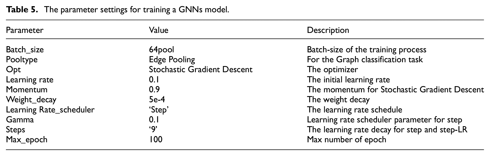
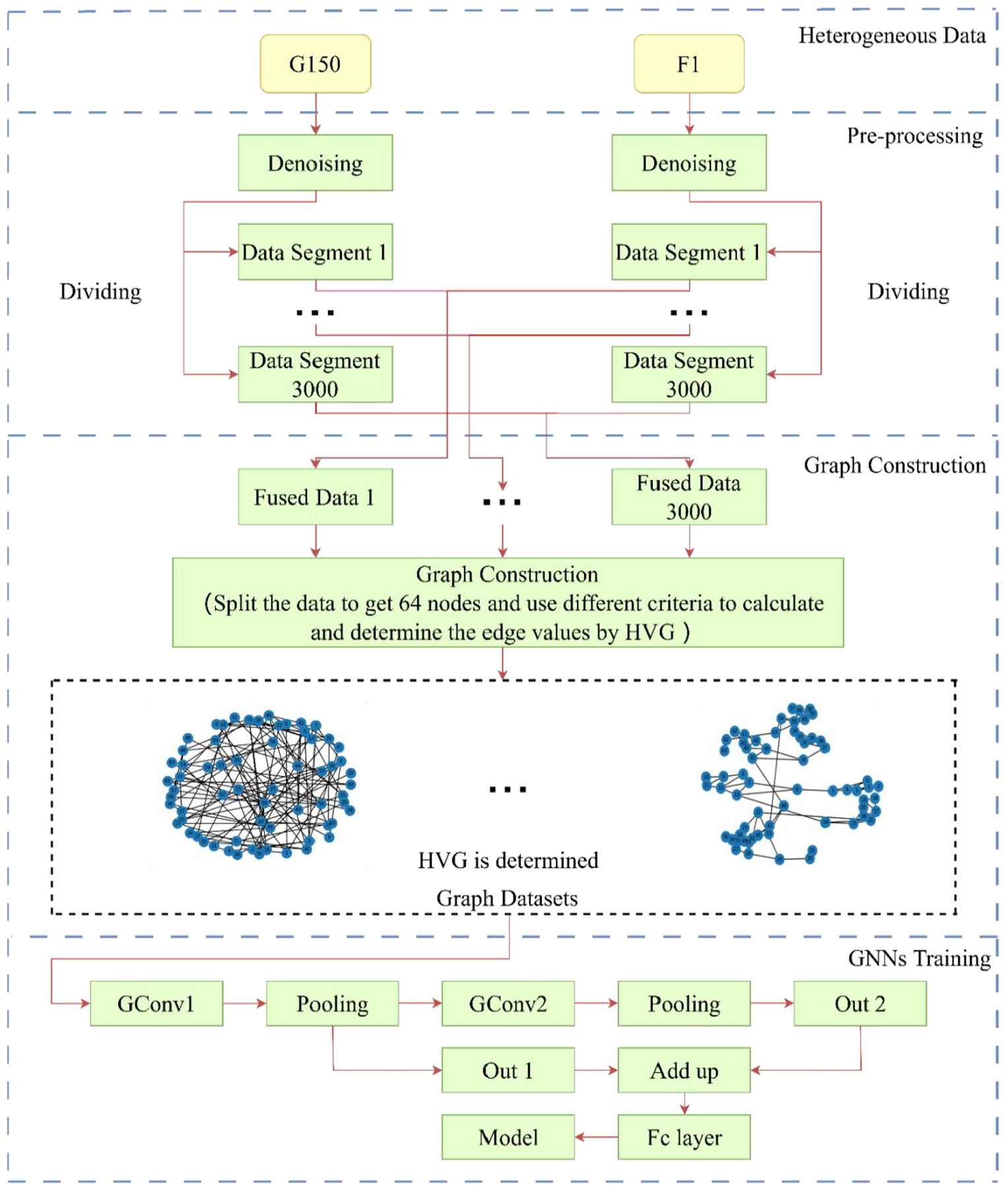
Figure 1 depicts a data fusion layer that integrates multiple GNNs, allowing each GNNs to analyze and interpret input data from its own perspective. Each GNNs may have a different focus, such as time-series patterns or spatial distribution characteristics. The features extracted by each GNNs are aggregated in the data layer via parallel processing, leading to a comprehensive evaluation result that encompasses a multi-faceted understanding of the mechanical seal system’s complex state. This methodology significantly enhances the accuracy and reliability of the evaluation. Firstly, the heterogeneous data, which come from different sensors, are collected. Secondly, after de-noising, the data would be divided as several segments. Thirdly, the different segments would be combined as the new fused data. Fourthly, the graph datasets could be constructed by using a graph construction method for each fused data. Obviously, the graph datasets are different if choosing different graph construction methods. Taking GSTFT as example, a fused data would be split as n sub-division, the n is number of nodes of graph. The STFT of each sub-division would be analyzed and the distance of STFT for each sub-division would be calculated, the distance value is the edge of two nodes for graph. If the distance of two nodes below the threshold, the edge could be ignored. Finally, the GNNs model would be trained by using the graph datasets. The structure of GNNs was designed in Li et al.¹³ The GNNs contains two pooling layers, two GConv layers with a fully connected layer. The pooling methods of choice are four methods such as “TopKPool,”“EdgePool,”“ASAPool,”“SAGPool.” Learning rate program options four ways including “step,”“exp,”“stepLR,”“fix.” By adding the output of the first pooling with the output of the second pooling through a fully connected layer. In our study, we utilize four graph data construction methods, as detailed in Table 1. A key aspect of our approach is the ability to fuse information from multiple sensor types during graph construction.

Figure 1.

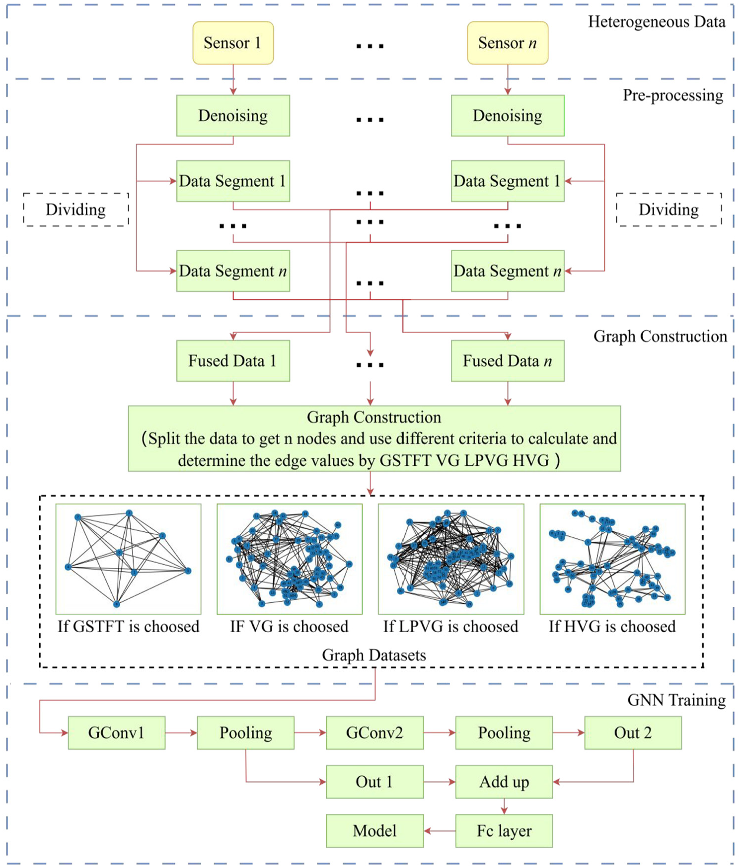
The structure of GNNs with fusing multi-sensor channels.

Table 1.

Four graph construction methods.

Method	Description
GSTFT	Constructing the graph based on STFT
VG	Using the visibility criteria to construct the graph data
HVG	Using the horizontal visibility criteria to construct the graph data
LPVG	Using the limited penetrable visibility criteria to construct the graph data

Thus, an assessment procedure for mechanical seals is proposed, as illustrated in Figure 2. This procedure consists of two main stages: the training stage and the testing stage. In the training stage, the initial step involves processing the raw data collected via multi-sensor arrays, which includes tasks such as outlier removal. Next, the original signal waveforms are transformed into graph data, which are then used to construct the training datasets. Finally, by integrating multiple GNNs with these datasets, an evaluation model is developed. The data gathered from these sensors are subsequently transformed into graph representations using methodologies aligned with the established assessment model. This leads to the generation of the assessment results. Additionally, in cases where the operational conditions are abnormal, the extent of damage to the mechanical seal can also be assessed.

Figure 2.

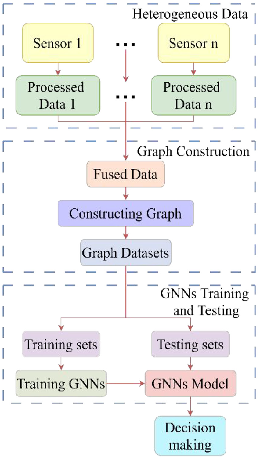
The flowchart of fault diagnosis based on GNNs with fusing multi-sensor channels.

Test, results, and discussion

Test rig and simulated faults

The test mechanical seal is shown in Figure 3. The test mechanical seal mainly comprises four parts, stationary ring, rotating ring, spring, and secondary seals. The secondary seals are used between the rotating component and shaft and between the stationary ring and gland plate. The spring provides the preload force between stationary ring and rotating ring to maintain the contact of each other. The seal faces, which consist of stationary ring and rotating ring, restrict leakage by operating in close proximity to one another. Any leakage through the seal assembly must be through the interface between the two faces which is known as face gap.

Figure 3.

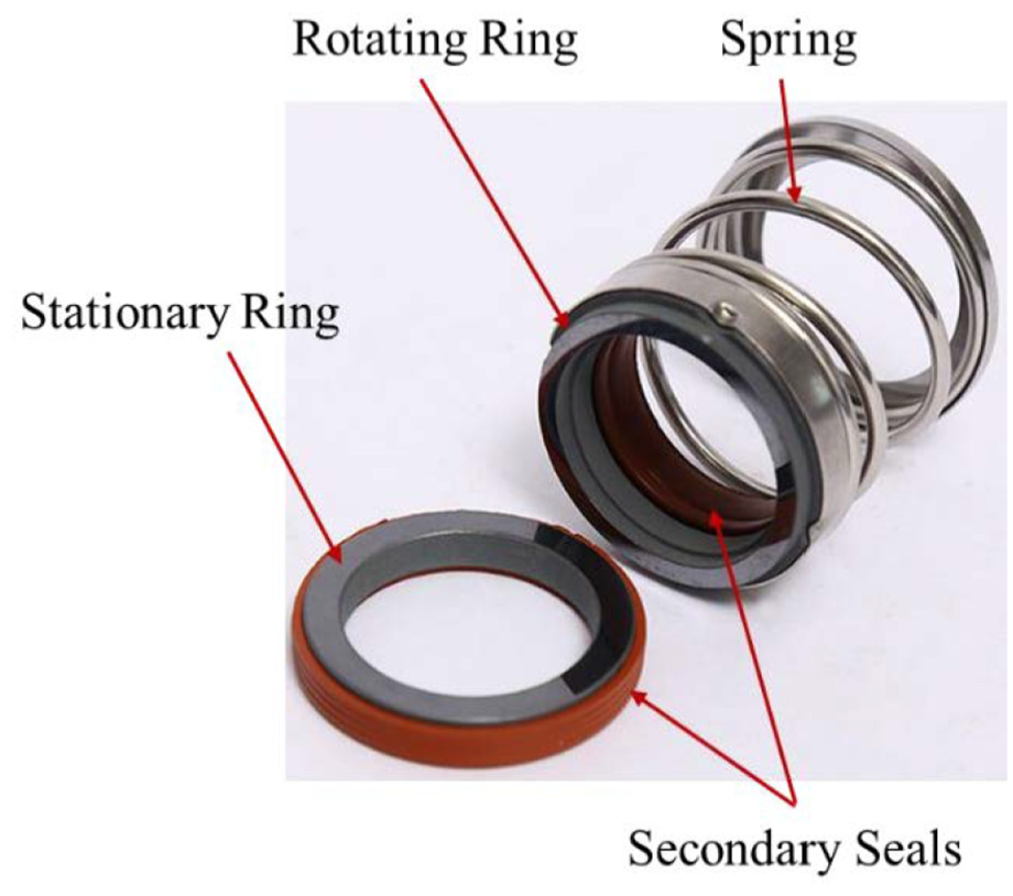
The test mechanical seal.

In order to monitor the condition of seal face of the mechanical seal, a test rig of mechanical seal is designed and manufactured, as shown in Figure 4. The test mechanical seal is mounted in the chamber. In order to measure the preload force of mechanical seal, a sensor ring, which consist of four force sensors (F1, F2, F3, F4), is mounted on back of the stationary ring. One Acoustic Emission (AE) sensor (GM150) directly measure the running data of seal face, the other AE sensor (G150) measure the overall running data of mechanical seal. The sampling rate and sampling points of AE sensor are 1 MHz and 1 M respectively, the sampling rate and sampling points of force sensor are 3.2 kHz and 3.2 K respectively.

Figure 4.

The test rig of mechanical seal: (a) the perspective of chamber for test rig of mechanical seal, (b) the arrange of sensors for test rig of mechanical seal, and (c) the overall for test rig of mechanical seal.

In order to simulate the faults of mechanical seal, the grooves are processed for RR and SR by using laser. The width of grooves included two types, 0.1 and 0.3 mm, as shown in Figure 5. And then, the test datasets are generated, as shown in Table 2.

Figure 5.

Simulated faults for rotating ring and stationary ring: (a) RR@0.1, (b) SR@0.1, (c) RR@0.3, and (d) SR@0.3.

Table 2.

Description of the test datasets.

Condition	Fault location	Fault dimension (mm)	Rotating speed (r/min)	Data size	Label
Normal			1000	3000	0
SR@0.1	Stationary ring	0.1	1000	3000	1
RR@0.1	Rotating ring	0.1	1000	3000	2
SR@0.3	Stationary ring	0.3	1000	3000	3
RR@0.3	Rotating ring	0.3	1000	3000	4

Signal processing results and graph data

Taking G150 and F1 as example, five data are extracted from five different running conditions, the signal processing results are shown as follow. In the meantime, the graphs, which fuse G150 and F1, are constructed by using four different methods as shown too.

Normal condition

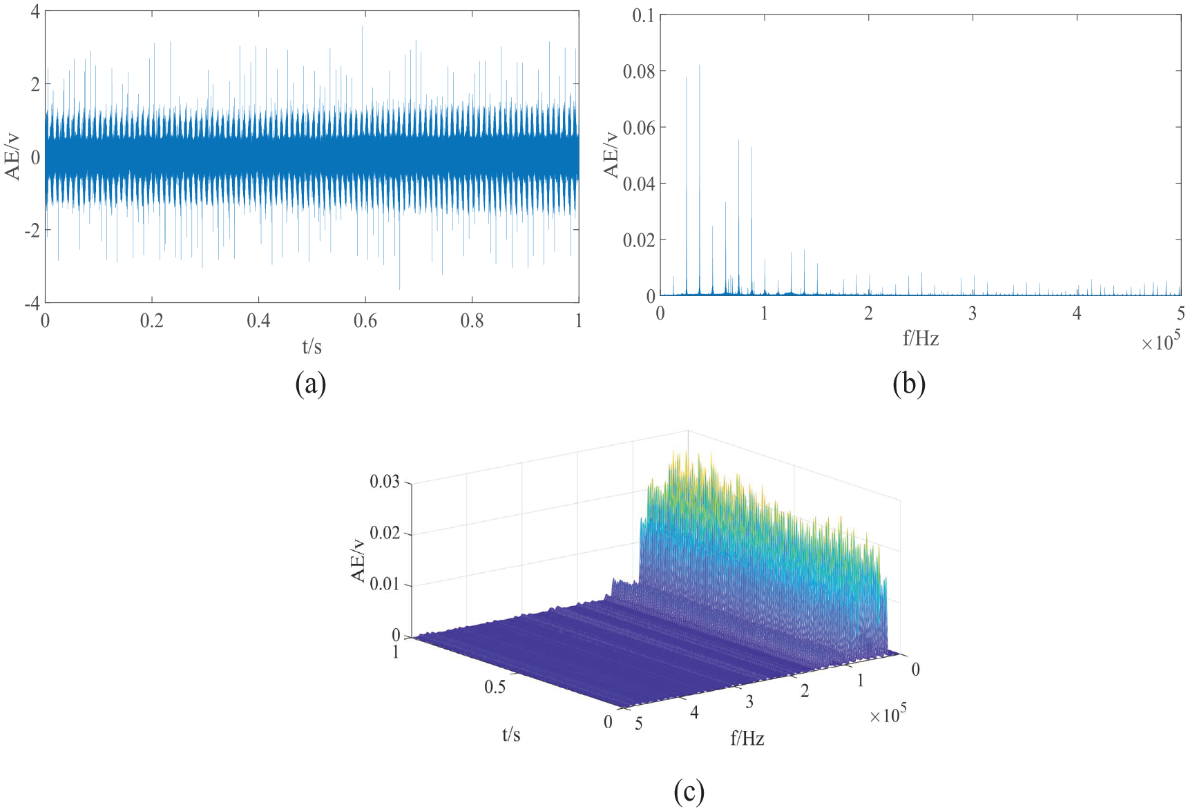
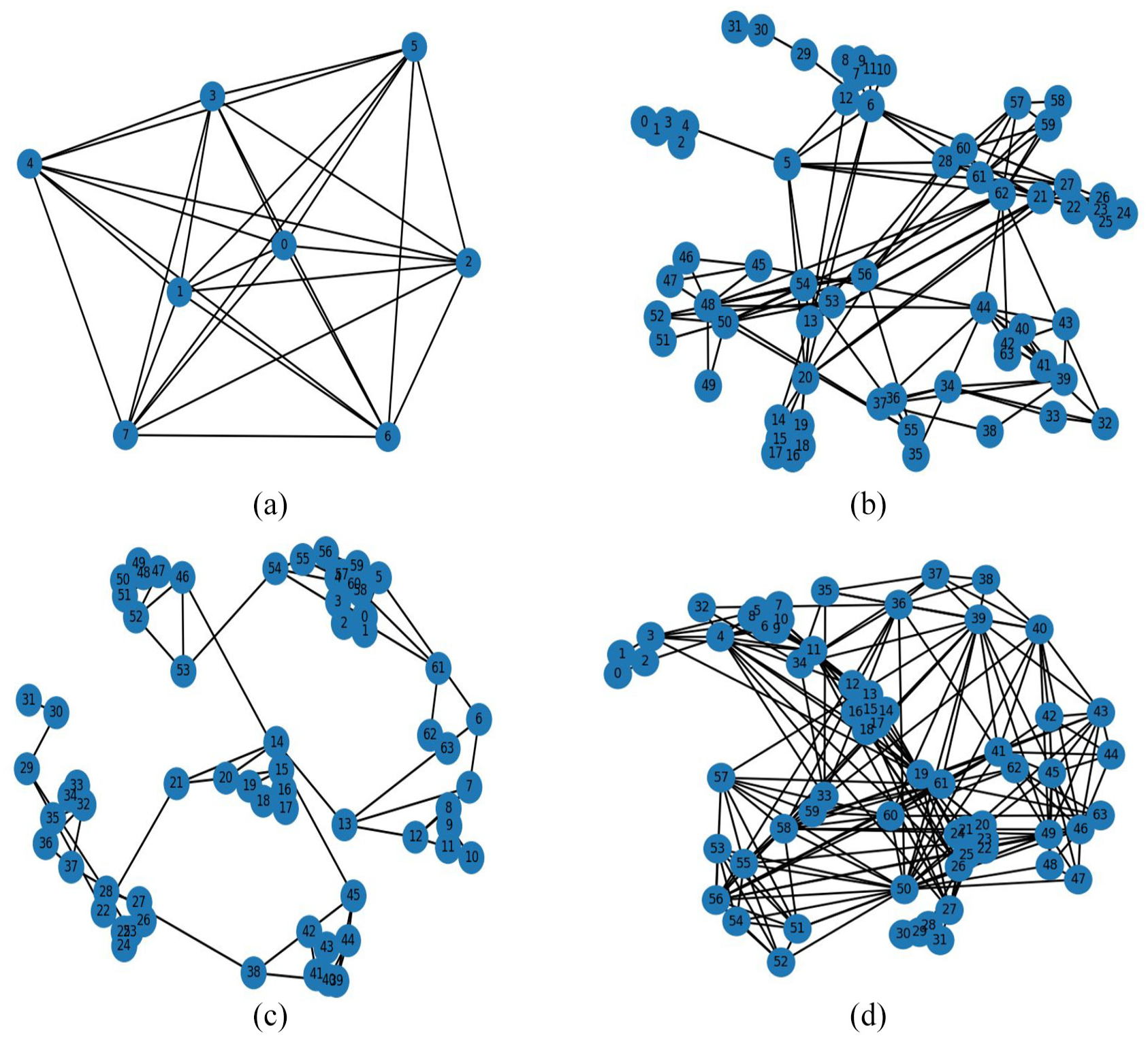
The raw waveform, FFT, and STFT of the G150 sensor display the characteristics under normal operating conditions. The original waveform, FFT, and STFT of the F1 force sensor also display the spectral characteristics during normal operation. Figures 6 to 8 shows these signals processing results, and the data of G150 and F1 were fused and constructed into graphical data using four methods: GSTFT, VG, HVG, and LPVG.

Figure 6.

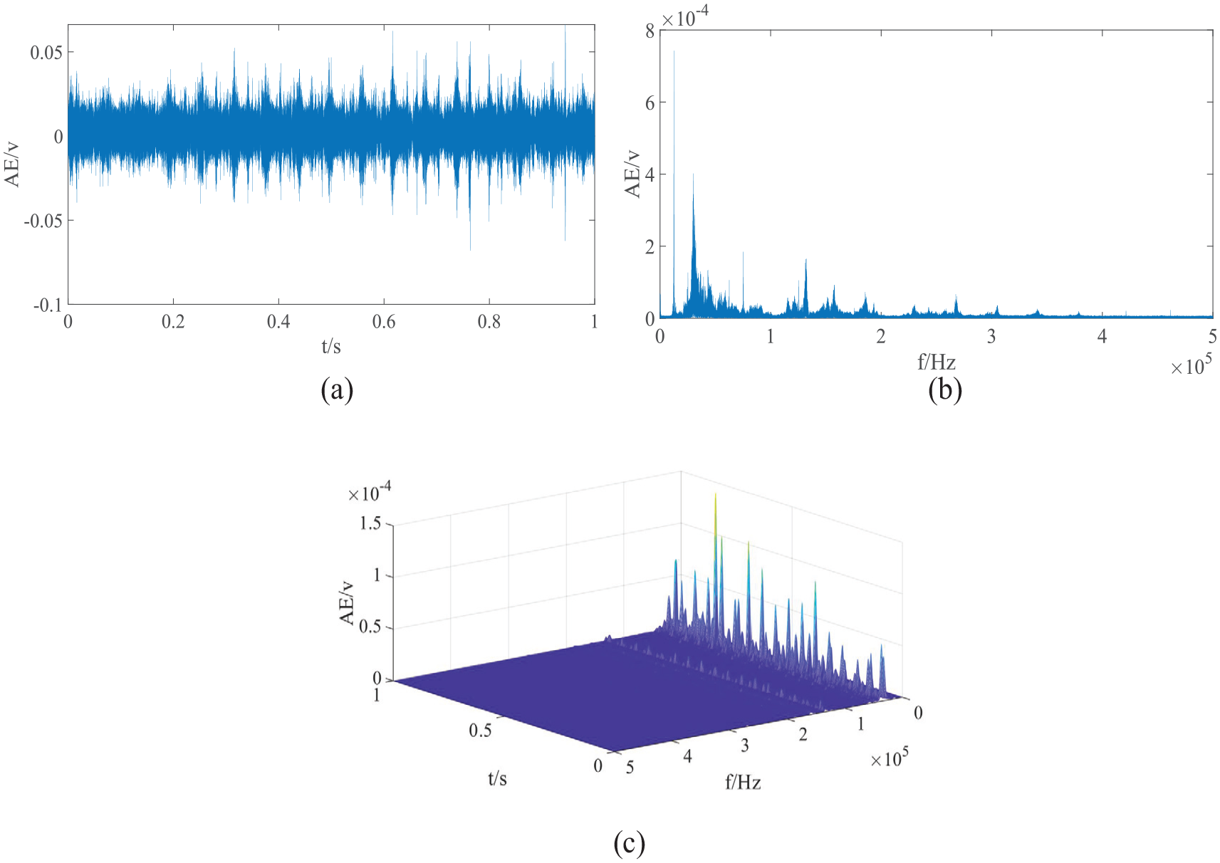
(a) Original wave of G150 for normal condition, (b) FFT of G150 for normal condition, and (c) STFT of G150 for normal condition.

Figure 7.

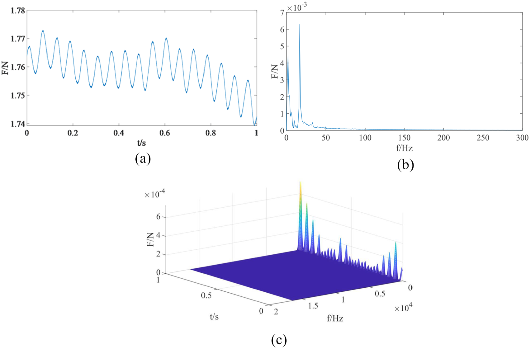
(a) Original wave of F1 for normal condition, (b) FFT of F1 for normal condition, and (c) STFT of F1 for normal condition.

Figure 8.

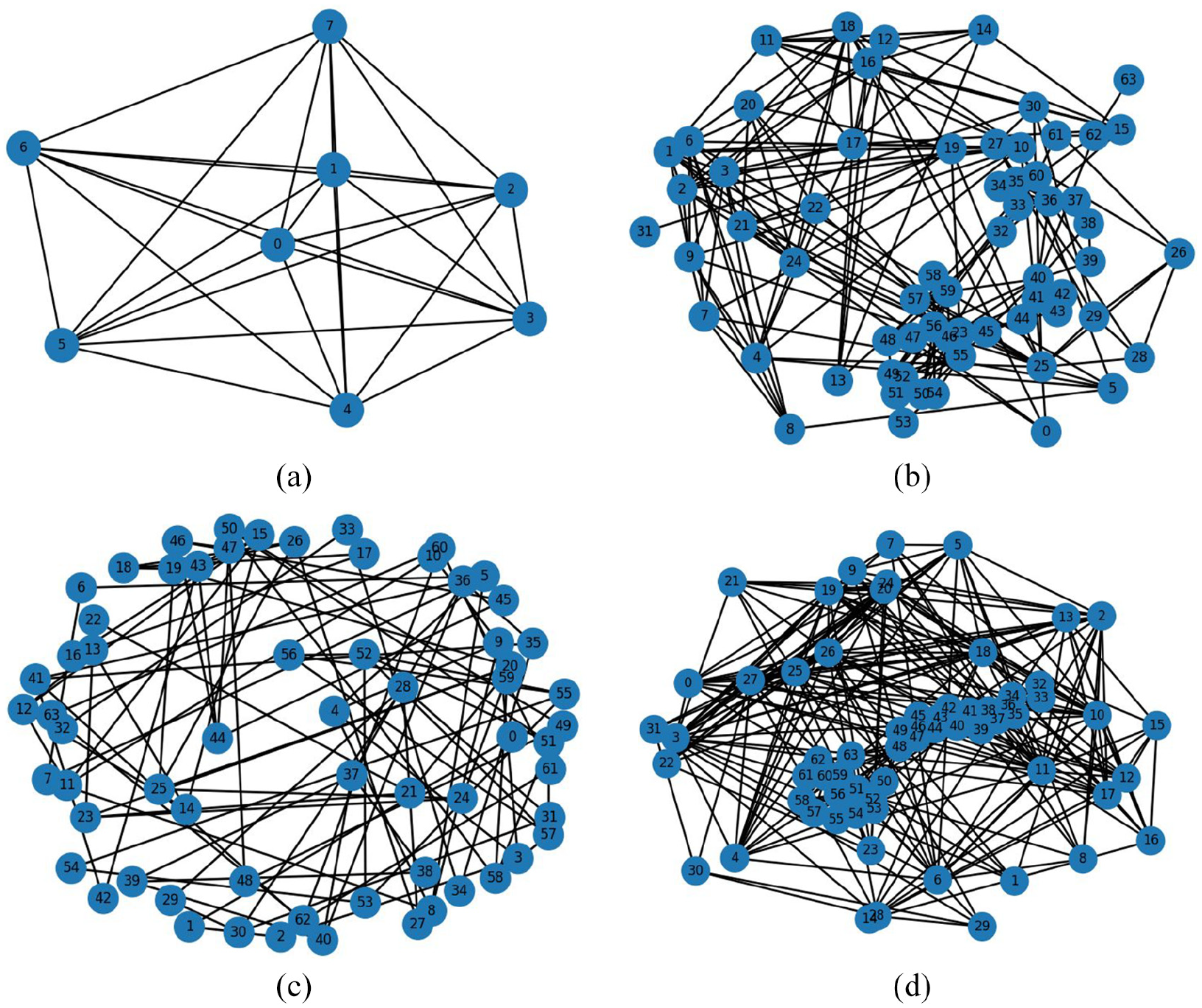
Graph of fusing G150-F1 for normal condition: (a) GSTF, (b) VG, (c) HVG, and (d) LPVG.

RR@0.1 condition

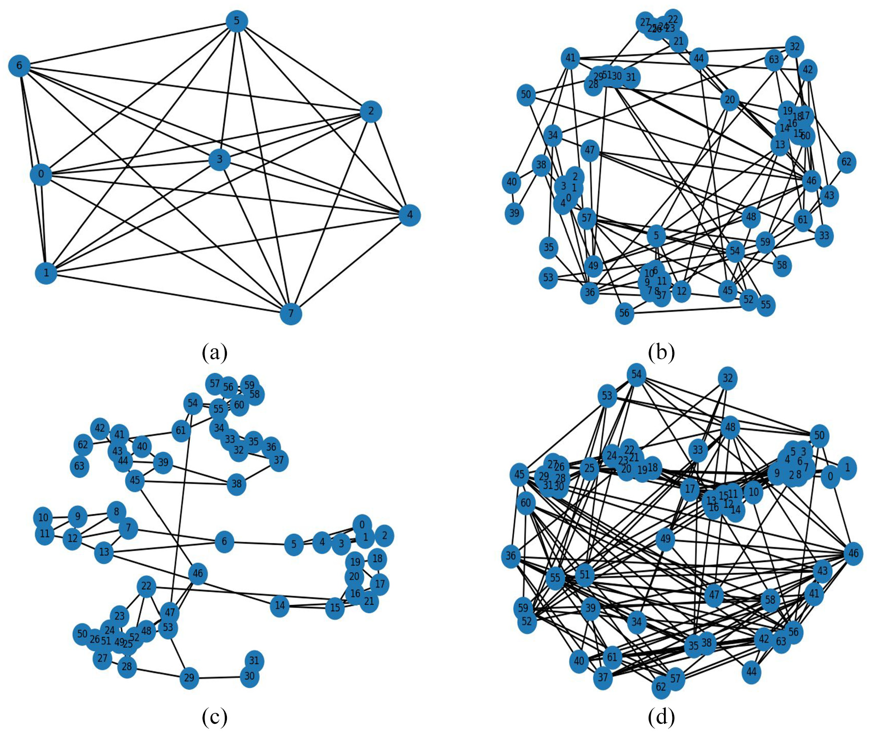
The raw waveforms, FFT, and STFT of G150 and F1 sensors exhibit characteristics that differ from normal operating conditions. Figures 9 to 11 show the signal processing results.

Figure 9.

(a) Original wave of G150 for RR@0.1 condition, (b) FFT of G150 for RR@0.1 condition, and (c) STFT of G150 for RR@0.1 condition.

Figure 10.

(a) Original wave of F1 for RR@0.1 condition, (b) FFT of F1 for RR@0.1 condition, and (c) STFT of F1 for RR@0.1 condition.

Figure 11.

Graph of fusing G150-F1 for RR@0.1 condition: (a) GSTFT, (b) VG, (c) HVG, and (d) LPVG.

SR@0.1 condition

G150 sensor: raw waveform, FFT and STFT displayed SR@0.1 Characteristics under certain conditions. F1 force sensor: The original waveform, FFT, and STFT are also displayed SR@0.1 Characteristics under certain conditions. Construction methods for Figures 12 to 14: Use GSTFT, VG, HVG, and LPVG to fuse the data of G150 and F1 and construct them into graphical data.

Figure 12.

(a) Original wave of G150 for SR@0.1 condition, (b) FFT of G150 for SR@0.1 condition, and (c) STFT of G150 for SR@0.1 condition.

Figure 13.

(a) Original wave of F1 for SR@0.1 condition, (b) FFT of F1 for SR@0.1 condition, and (c) STFT of F1 for SR@0.1 condition.

Figure 14.

Graph of fusing G150-F1 for SR@0.1 condition: (a) GSTFT, (b) VG, (c) HVG, and (d) LPVG.

RR@0.3 condition

G150 sensor: The raw waveform, FFT, and STFT show more significant differences from normal operating conditions. F1 force sensor: The original waveform, FFT, and STFT also showed more significant differences compared to normal operating conditions. Figures 15 to 17 construction method: Use GSTFT, VG, HVG, and LPVG to fuse the data of G150 and F1 and construct them into graphical data.

Figure 15.

(a) Original wave of G150 for RR@0.3 condition, (b) FFT of G150 for RR@0.3 condition, and (c) STFT of G150 for RR@0.3 condition.

Figure 16.

(a) Original wave of F1 for RR@0.3 condition, (b) FFT of F1 for RR@0.3 condition, and (c) STFT of F1 for RR@0.3 condition.

Figure 17.

Graph of fusing G150-F1 for RR@0.3 condition: (a) GSTFT, (b) VG, (c) HVG, and (d) LPVG.

SR@0.3 condition

G150 sensor: The raw waveform, FFT, and STFT show more significant differences from normal operating conditions. F1 force sensor: Especially the F1 force sensor SR@0.3. The STFT results under certain conditions exhibit unique features that can be used to identify the presence and extent of damage. Figures 18 to 20 construction method: Use GSTFT, VG, HVG, and LPVG to fuse the data of G150 and F1 and construct them into graphical data.

Figure 18.

(a) Original wave of G150 for SR@0.3 condition, (b) FFT of G150 for SR@0.3 condition, and (c) STFT of G150 for SR@0.3 condition.

Figure 19.

(a) Original wave of F1 for SR@0.3 condition, (b) FFT of F1 for SR@0.3 condition, and (c) STFT of F1 for SR@0.3 condition.

Figure 20.

Graph of fusing G150-F1 for SR@0.3 condition: (a) GSTFT, (b) VG, (c) HVG, and (d) LPVG.

Raw waveforms

Figure 6(a) shows the raw waveform of AE sensor G150 under normal operating conditions. It can be seen that the waveform is relatively smooth with no obvious abnormal fluctuations or spikes, which indicates that the mechanical sealing system operates stably under normal operating conditions without any significant failure.

FFT diagram

Figure 6(b) shows the FFT plot of the G150 sensor under normal operating conditions. The FFT plot shows that the main frequency components of the signal are concentrated in the lower frequency band and the amplitude is small. This indicates that under normal operating conditions, there are low levels of vibration and noise in the system and no obvious sources of periodic faults.

STFT plot

Figure 6(c) shows the STFT plot of the G150 sensor under normal operating conditions. The STFT plot demonstrates how the frequency of the signal changes at different points in time. It can be seen that the frequency component of the signal remains relatively stable over time, with no significant time-varying characteristics. This further verifies the stability of the system under normal operating conditions.

Figure 8(a) illustrates the graph structure that was constructed by fusing the data from the G150 and F1 sensors using the GSTFT method, which is based on time-frequency domain information and is capable of capturing the local characteristics of the signals. Under normal operating conditions, the nodes in the graph are more sparsely connected and the weights of the edges are smaller, which reflects the simpler interactions between the sensors in the system without complex dependencies.

Diagnostic results

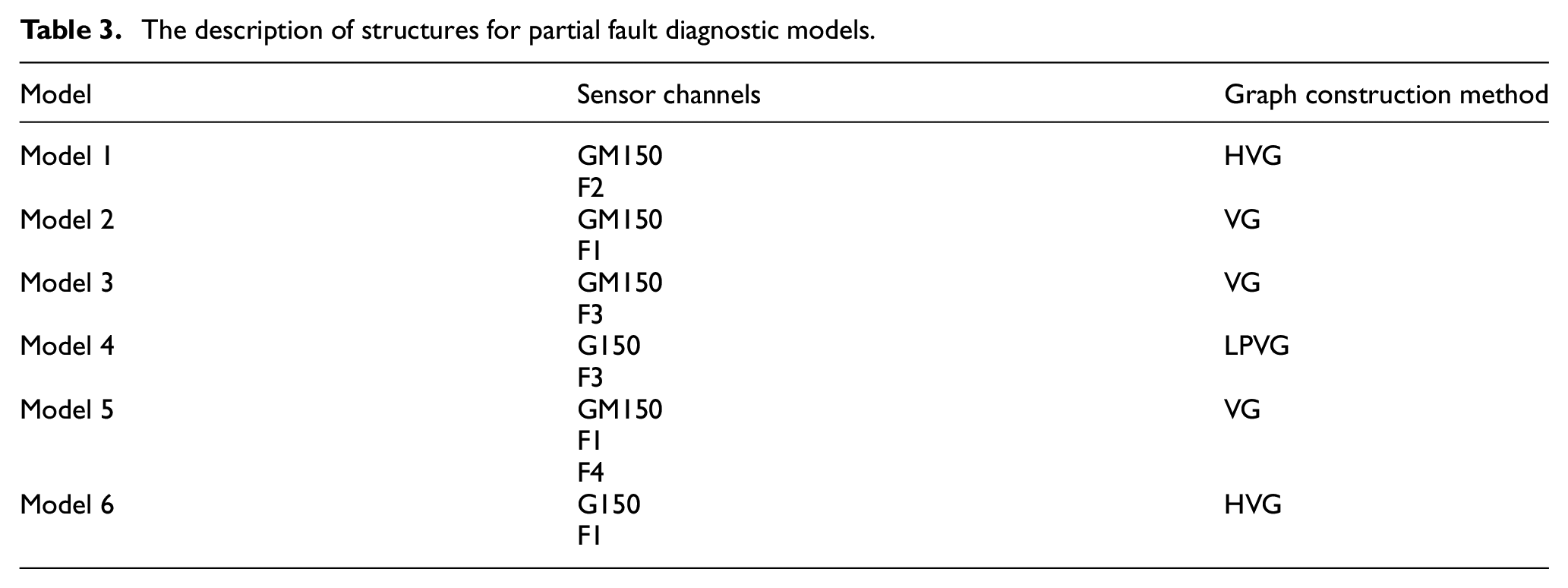
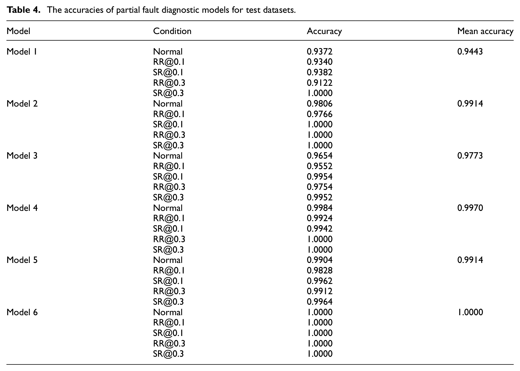
Due to the extensive number of possible combinations involving multi-sensor data, various graph data construction methods, and different fusion strategies, only a subset of the assessment models is presented in Table 3. The evaluations of these selected models are detailed in Table 4. The parameter settings for training a GNNs model are shown in Table 5.

Table 3.

The description of structures for partial fault diagnostic models.

Model	Sensor channels	Graph construction method
Model 1	GM150	HVG
Model 1	F2	HVG
Model 2	GM150	VG
Model 2	F1	VG
Model 3	GM150	VG
Model 3	F3	VG
Model 4	G150	LPVG
Model 4	F3	LPVG
Model 5	GM150	VG
	F1
	F4
Model 6	G150	HVG
Model 6	F1	HVG

Table 4.

The accuracies of partial fault diagnostic models for test datasets.

Model	Condition	Accuracy	Mean accuracy
Model 1	Normal	0.9372	0.9443
	RR@0.1	0.9340
	SR@0.1	0.9382
	RR@0.3	0.9122
	SR@0.3	1.0000
Model 2	Normal	0.9806	0.9914
	RR@0.1	0.9766
	SR@0.1	1.0000
	RR@0.3	1.0000
	SR@0.3	1.0000
Model 3	Normal	0.9654	0.9773
	RR@0.1	0.9552
	SR@0.1	0.9954
	RR@0.3	0.9754
	SR@0.3	0.9952
Model 4	Normal	0.9984	0.9970
	RR@0.1	0.9924
	SR@0.1	0.9942
	RR@0.3	1.0000
	SR@0.3	1.0000
Model 5	Normal	0.9904	0.9914
	RR@0.1	0.9828
	SR@0.1	0.9962
	RR@0.3	0.9912
	SR@0.3	0.9964
Model 6	Normal	1.0000	1.0000
	RR@0.1	1.0000
	SR@0.1	1.0000
	RR@0.3	1.0000
	SR@0.3	1.0000

Table 5.

The parameter settings for training a GNNs model.

Parameter	Value	Description
Batch_size	64pool	Batch-size of the training process
Pooltype	Edge Pooling	For the Graph classification task
Opt	Stochastic Gradient Descent	The optimizer
Learning rate	0.1	The initial learning rate
Momentum	0.9	The momentum for Stochastic Gradient Descent
Weight_decay	5e-4	The weight decay
Learning Rate_scheduler	‘Step’	The learning rate schedule
Gamma	0.1	Learning rate scheduler parameter for step
Steps	‘9’	The learning rate decay for step and step-LR
Max_epoch	100	Max number of epoch

Discussion

Comparison of signal processing results

The signal processing techniques applied to the sensor data revealed distinctive patterns corresponding to the normal, damage to the SR, and damage to the RR of the mechanical seal. For instance, the STFT of force sensor F1 data under the SR@0.3 condition (Figures 19 and 20) showed unique features that could be utilized to identify the presence and severity of the fault. These results indicate that different types of damage manifest in characteristic ways, making it possible to distinguish between various fault conditions.

Comparison of methods for constructing graph data

Four different methods were employed to construct graph data from the sensor readings:

(1) GSTFT: Utilizes the temporal-frequency domain information to create graph structures.

(2) VG: Constructs the graph using the visibility criteria, converting time series data into a graph where the visibility properties of the data points define the edges.

(3) HVG: Similar to VG but uses horizontal visibility criteria, which simplifies the graph construction process while preserving meaningful relationships.

(4) LPVG: Combines elements of both VG and HVG, offering a balance between simplicity and complexity, and potentially improving the model’s interpretability.

(5) Each graph construction method provided a unique perspective on the sensor data, and the results showed that the choice of construction method influenced the performance of the GNNs. For example, the HVG method seemed to work well with the Model 6 configuration, achieving high accuracy across all conditions tested (Table 4).

Comparison of model structure and classification accuracy

The models varied in terms of sensor channels used, graph construction methods, and fusion strategies, leading to differences in classification accuracy. Notably, the fusion of multiple GNNs through a data fusion layer (Figure 1) improved the overall accuracy and robustness of the assessment.

(1) Model 1 (GM150 + HVG + F2) achieved a mean accuracy of 0.9443, demonstrating the effectiveness of the HVG method combined with the AE sensor GM150 and force sensor F2.

(2) Model 2 (GM150 + VG + F1) had a higher mean accuracy of 0.9914, suggesting that the VG method paired with the AE sensor GM150 and force sensor F1 was particularly effective.

(3) Model 4 (G150 + LPVG + F3) achieved the highest mean accuracy of 0.9971, indicating that the LPVG method with AE sensor G150 and force sensor F3 was the most successful among the models tested.

(4) Model 6 (G150 + HVG + F1) achieved perfect accuracy across all conditions, making it the best-performing model in the study.

Overall, the models that incorporated the LPVG and HVG methods tended to perform better, possibly due to their ability to capture both the temporal and spatial characteristics of the sensor data more effectively. Additionally, as shown in Figure 21, the fusion of multiple sensor channels and the use of different graph construction methods allowed the models to capture the complex dynamics of the mechanical seal system, leading to enhanced classification accuracy.

Figure 21.

The structure of the best fault diagnostic model.

Conclusions

The new assessment model and process for mechanical seals, which leverage the fusion of multi-GNNs, are introduced. The key findings are summarized as follows:

(1) Signal processing results reveal distinct patterns for normal operation, damage to the stationary ring, and damage to the rotating ring.

(2) Different degrees of damage to the stationary and rotating rings exhibit unique characteristics.

(3) Sensor channels, comprising two Acoustic Emission (AE) sensors (G150 and GM150) and four force sensors (F1, F2, F3, F4), provide partial but diverse insights into the operational state of the mechanical seal.

(4) Beyond the inherent diversity among sensor channels, the use of various Graph Data Construction Methods further enriches this diversity.

(5) This diversity is inherited by the GNNs trained on different datasets, leading to varied network structures. The fusion of these multi-GNNs enhances the overall accuracy of the assessment.

(6) The evaluation outcomes demonstrate that the integrated assessment model, which combines multiple GNNs, can accurately determine the condition of mechanical seals.

Footnotes

Handling Editor: Divyam Semwal

Author contributions

Xiaoran Zhu: Funding acquisition, Supervision, Conceptualization, Methodology, Writing-review & editing, Data curation. Jiahao Wang: Software, Data curation. Binhui Wang: Writing-original draft, Software, Data curation. Hao Wang: Software. Ren Sheng: Review & editing. Baozun Zhai: Funding acquisition, Review & editing.

Declaration of conflicting interests

The author(s) declared no potential conflicts of interest with respect to the research, authorship, and/or publication of this article.

Funding

The author(s) disclosed receipt of the following financial support for the research, authorship, and/or publication of this article: This research is supported by the Project of Science and Technology of Henan (No. 222102220115). Key Research Project of Universities in Henan Province (Project No. 24A413004).

ORCID iD

Xiaoran Zhu

References

Sun

. Thermomechanical coupled analysis of split mechanical seal under different rotation speeds. Adv Mech Eng 2016; 8: 1–13.

Tang

Xiao

Yang

, et al. Research on a small sample feature transfer method for fault diagnosis of reciprocating compressors. J Loss Prev Process Ind 2023; 85: 105163.

Zhou

Xue

, et al. A rotating machinery fault diagnosis method based on dynamic graph convolution network and hard threshold denoising. Sensors 2024; 24: 4887.

Yao

Chang

Han

, et al. Semi-supervised adversarial deep learning for capacity estimation of battery energy storage systems. Energy 2024; 294: 130882.

Liu

Guo

, et al. A collaborative central domain adaptation approach with multi-order graph embedding for bearing fault diagnosis under few-shot samples. Appl Soft Comput 2023; 140: 110243.

Lei

Yang

Jiang

, et al. Applications of machine learning to machine fault diagnosis: a review and roadmap. Mech Syst Signal Process 2020; 138: 1–39.

Pan

Chen

, et al. A comprehensive survey on graph neural networks. IEEE Trans Neural Netw Learn Syst 2021; 32: 4–24.

Zhou

Huo

Hou

, et al. Co-embedding of edges and nodes with deep graph convolutional neural networks. Sci Rep 2023; 13: 16966.

Yan

. XGBoost-enhanced graph neural networks: a new architecture for heterogeneous tabular data. Appl Sci 2024; 14: 5826.

10.

Zhang

Cui

Neumann

, et al. An end-to-end deep learning architecture for graph classification. Proc AAAI Conf Artif Intell 2018; 544: 4438–4445.

11.

Zhang

, et al. Semi-supervised classification of graph convolutional networks with Laplacian rank constraints. Neural Process Lett 2021; 54: 2645–2656.

12.

Scarselli

Gori

Tsoi

, et al. The graph neural network model. IEEE Trans Neural Netw 2009; 20: 61–80.

13.

Zhou

, et al. The emerging graph neural networks for intelligent fault diagnostics and prognostics: a guideline and a benchmark study. Mech Syst Signal Process 2022; 168: 108653.

14.

Cao

Chen

, et al. Graph neural network architecture search for rotating machinery fault diagnosis based on reinforcement learning. Mech Syst Signal Process 2023; 202: 110701.

15.

Hassani

Dackermann

Mousavi

, et al. A systematic review of data fusion techniques for optimized structural health monitoring. Inf Fusion 2024; 103: 102136.

16.

Zhou

Zhang

, et al. Bayesian differentiable architecture search for efficient domain matching fault diagnosis. IEEE Trans Instrum Meas 2021; 70: 1–11.

17.

Zhao

Sun

, et al. Hierarchical attention graph convolutional network to fuse multi-sensor signals for remaining useful life prediction. Reliab Eng Syst Saf 2021; 215: 107878.

18.

Fan

Ball

. A review of the condition monitoring of mechanical seals. In: ASME 7th Biennial conference on engineering systems design and analysis, Manchester, UK, 19–22 July 2004, pp.179–184. New York: ASME.

19.

Fan

Ball

. Acoustic emission monitoring of mechanical seals using MUSIC algorithm based on higher order statistics. Key Eng Mater 2009; 413: 811–816.

20.

Fan

Ball

. Modelling acoustic emissions generated by sliding friction. Wear 2010; 268: 811–815.

21.

Towsyfyan

Ball

, et al. Modelling acoustic emissions generated by tribological behaviour of mechanical seals for condition monitoring and fault detection. Tribol Int 2018; 125: 46–58.

22.

Towsyfyan

Ball

, et al. Tribological behaviour diagnostic and fault detection of mechanical seals based on acoustic emission measurements. Friction 2019; 7: 572–586.

23.

Kipf

Welling

. Semi-supervised classification with graph convolutional networks. arXiv preprint arXiv:1609.02907, 2016.

24.

Veličković

Cucurull

Casanova

, et al. Graph attention networks. OpenReview.net, 2018. DOI: 10.17863/CAM.48429.

25.

Goyal

Pabla

. Condition based maintenance of machine tools-a review. CIRP J Manuf Sci Technol 2015; 10: 24–35.

26.

Lacasa

Luque

Ballesteros

, et al. From time series to complex networks: the visibility graph. Appl Math 2008; 105: 4972–4975.

27.

Luque

Lacasa

Ballesteros

, et al. Horizontal visibility graphs: exact results for random time series. arXiv preprint arXiv:1002.4526, 2010.

28.

Zhou

Jin

Gao

, et al. Limited penetrable visibility graph for establishing complex network from time series. Acta Phys Sin 2012; 61: 030506.

Fault diagnosis of mechanical seals using graph neural networks with multi-sensor data fusion

Abstract

Keywords

Introduction

Graph neural networks

Fault diagnosis method based on GNNs with fusing multi-sensor channels

Test, results, and discussion

Test rig and simulated faults

Signal processing results and graph data

Normal condition

RR@0.1 condition

SR@0.1 condition

RR@0.3 condition

SR@0.3 condition

Raw waveforms

FFT diagram

STFT plot

Diagnostic results

Discussion

Comparison of signal processing results

Comparison of methods for constructing graph data

Comparison of model structure and classification accuracy

Conclusions

Footnotes

Author contributions

Declaration of conflicting interests

Funding

ORCID iD

References