Sage Journals: Discover world-class research

Abstract

Accurate sand control design requires that the sand particles that break through the sand control facilities and enter the wellbore can be completely transported to the wellhead to prevent wellbore sand settling and blocking. At present, there are few studies on the migration and deposition of formation sand with a certain particle size distribution (PSD) after entering the wellbore with formation fluid. Most studies do not consider the sand PSD and treat sand particles as pseudo fluid. Therefore, this paper uses CFD-DEM (computational fluid dynamics-discrete element method) coupling method to conduct numerical simulation of sand migration in the wellbore, and obtains the influence rule of fluid velocity, viscosity, well deviation angle, formation sand production concentration, and PSD on cross-section sand concentration (sand carrying capacity of the fluid) and axial pressure drop in the wellbore section. Based on the simulation results and dimensional analysis, a prediction model for the volume concentration of sand particles in the wellbore was established, which is convenient for engineering applications to quickly determine the flow state of the wellbore. An engineering method for determining the critical non-deposition velocity of sand particles in wellbore was proposed, and the critical non-deposition velocity of sand particles under three effective particle sizes, three sand production concentrations, and three fluid viscosities was obtained. The research results can provide a theoretical basis for sand carrying and the production systems coordinated optimization design in weakly consolidated sandstone reservoirs.

Keywords

CFD-DEM fractal dimension of formation sand cross-section sand concentration critical non-deposition velocity

Introduction

70% of the world’s oil and natural gas reserves are weakly consolidated or unconsolidated sandstone reservoirs.^1–5 Due to the weak degree of cementation, changes in the geological conditions and production factors of oil and gas reservoirs during the development process cause changes in the rock structure, which leads to some rock particles being carried into the wellbore by formation fluids, resulting in sand production.^6–12 Despite the use of different methods for sand control, some formation sand is inevitably carried into the production system by the produced fluid, increasing wellbore pressure loss. The effective transportation of particles is crucial for production operations.^13–17

When using an independent mechanical screen for sand control, some of the formation sand smaller than the slot width will enter the wellbore with the produced fluid through the sand blocking medium. Accurate sand control design requirements should ensure that the sand particles entering the wellbore can be fully transported to the wellhead to prevent sand settling and blockage in the wellbore. The transportation process of formation sand from the reservoir to the ground is shown in Figure 1. The most challenging tasks of assessing the sand impacts on pipeline design are determining the particle sizes and determining the concentration of the sands that would be transported by the pipeline.

Figure 1.

Schematic diagram of sand migration from reservoir to wellbore.

Regarding the study of critical flow velocity, for single-phase fluid carrying sand in horizontal pipelines, Dabirian et al.^18,19 classified the particle motion state into homogeneous suspension (SB), heterogeneous suspension (Het), moving bed (MB), and stationary bed (SB). There are multiple definitions for the critical velocity of sand transport based on the different particle motion states. Durand²⁰ defines the minimum flow velocity without forming a stationary sand bed as the “ultimate sedimentation velocity” based on the principle of minimizing the loss of fluid kinetic energy; Oroskar and Turian²¹ and Davies²² defined the critical velocity as the minimum velocity at which sand particles remain suspended; Some scholars define the critical velocity as the fluid velocity corresponding to the transition from SB mode to MB mode; Najmi et al. defines the velocity at which solid particle suspension occurs in the flow as the critical flow velocity.²³ Soepyan et al.²⁴ defined five sand carrying velocities: the minimum velocity at which the sand bed at the bottom of the pipeline is suspended is the critical velocity; the fluid velocity at which the sand or gravel group resting above the sand bed can move with the fluid is the carrying velocity; the fluid velocity at which a single gravel stationary on the pipe wall moving with the fluid is called the starting velocity; the minimum flow velocity to ensure that the sand and gravel do not settle to the pipe wall during suspension is the jump velocity; the velocity at which the height of the sand bed in the pipeline remains stable is the equilibrium velocity.

The traditional sand carrying flow analysis mostly focuses on the two-fluid model to simulate the sand carrying law. The critical sand carrying velocity is determined by the single particle force analysis method.²⁵ The flow state of solid particles in the horizontal section of the oil well is calculated based on experimental data.²¹

Regarding the research of numerical models, particle group collision and accumulation are of great significance for studying the sand carrying mechanism in the wellbore. To model fluid–particle flows, scholars have developed continuum theory Euler–Euler and discrete medium theory Euler–Lagrange approaches and by considering particle as a quasi-fluid and discrete system based on the scale and mechanical characteristics of the research problem. DPM discrete phase model and TFM dual fluid model for computational fluid dynamics are widely used, but they cannot describe phenomena such as particle group collisions and stacking. The Euler–Lagrange approach considers a combination of computational fluid dynamics (CFD) and the discrete element method (DEM), referred as CFD-DEM. Due to its computational advantages over LB-DEM and DNS-DEM, as well as its ability to capture particle-particle interactions compared to TFM, the CFD-DEM method has been widely applied in various fields such as pipeline pneumatic conveying, fluidized bed, and dynamic simulation of wind and sand, reflecting the unique advantages of this coupled method.

The particle transport in multiphase flow is complex and depends on many factors, such as phase velocity, particle size, particle shape, particle concentration, particle density, pipe diameter, flow conditions, liquid viscosity and density, etc. Siamak proposed a coupled CFD-DEM method for predicting the migration behavior of rock cuttings considering dynamic collision processes.²⁶ Currently, this method has not been used for studying wellbore sand transport.^27,28 In recent years, CFD-DEM coupling system was developed to determine the collision among granules or between the granules and the wall. However, no numerical simulation of sand particle movement in the wellbore has been reported.

Accurately predicting the sand carrying flow state in the wellbore has important theoretical guidance significance for the efficient development of oil wells. Therefore, this paper has carried out the coupling theoretical research of CFD-DEM and its application in sand migration in two-phase flow, analyzed the flow law of sand carrying in the wellbore under different flow parameters, established the prediction model of sand volume concentration in the wellbore through dimensional analysis, and proposed a method to determine the critical non deposition velocity of sand in the wellbore, which provide a theoretical basis for the coordinated optimization design of wellbore sand carrying and production systems in weakly consolidated sandstone reservoirs.

Theoretical model of oil sand two-phase flow

Coupled dynamic model of two-phase flow

Taking fluid (oil) and particle (sand) in the wellbore as the research objects, the principle of momentum exchange in liquid-solid two-phase flow between grid units is shown in Figure 2.

Figure 2.

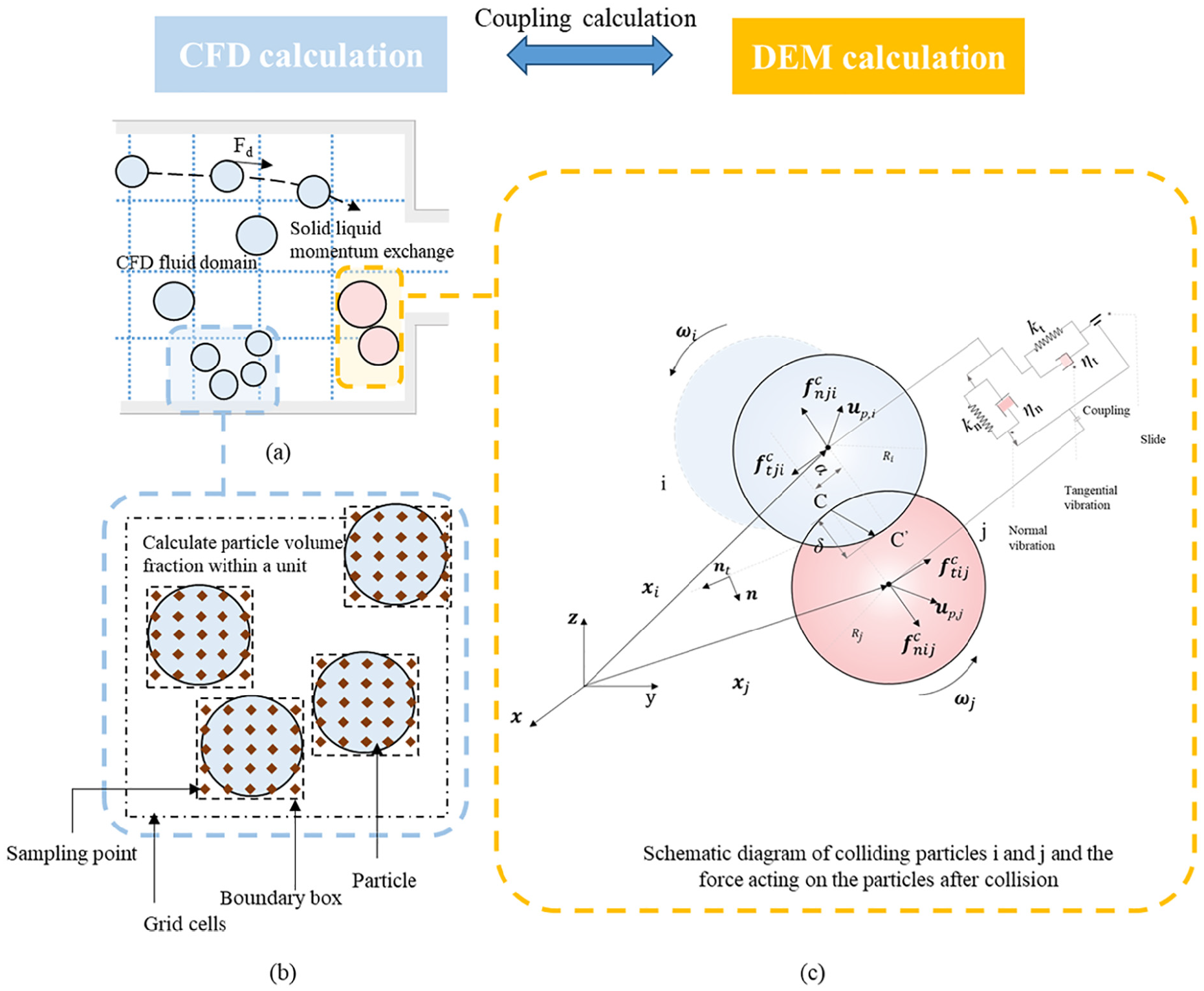
CFD-DEM coupling analysis process: (a) Coupled dynamic model of two-phase flow, (b) Enlarged image of sampling rules, (c) Enlarged image of particle collision.

Divide the model into solid particle domain $Ω_{p}$ and fluid domain $Ω_{f}$ . For the fluid domain $Ω_{f}$ , the velocity at the inlet boundary $Γ_{in}$ is $u_{Γ in, f}$ , the pressure at the outlet boundary $Γ_{out}$ is $p_{Γ in, f}$ , and the wall boundary $Γ_{int}$ (the flow region and wellbore coupling interface) is assumed to be non-slip, denoted by $u_{Γ I, f} = 0$ . Take the control volume $d V_{cell}$ , where the volumes of the liquid, solid are $d V_{f}$ and $d V_{p}$ respectively, and adopt momentum coupling strategy. The coupling parameters are $ε_{f}$ and source terms $F^{OM}$ , that is, the influence of the fluid domain on the solid phase is mainly reflected in the surface force of the fluid on the particle groups.

Oil control equation

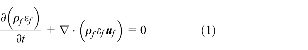
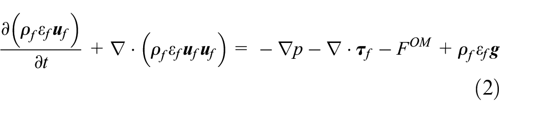
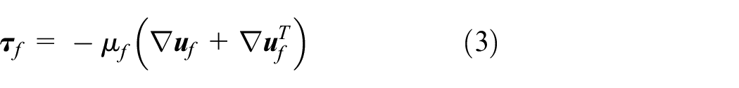
The control equation for the liquid phase oil is based on the Euler multiphase flow model: (in the formula, bold is a vector or tensor).

\frac{\partial (ρ_{f} ε_{f})}{\partial t} + \nabla \cdot (ρ_{f} ε_{f} u_{f}) = 0

(1)

\frac{\partial (ρ_{f} ε_{f} u_{f})}{\partial t} + \nabla \cdot (ρ_{f} ε_{f} u_{f} u_{f}) = - \nabla p - \nabla \cdot τ_{f} - F^{OM} + ρ_{f} ε_{f} g

(2)

τ_{f} = - μ_{f} (\nabla u_{f} + \nabla u_{f}^{T})

(3)

Where, $ε_{f}$ is the volume fraction of the liquid phase, dimensionless; $ρ_{f}$ is the liquid phase density, kg/m³; $u_{f}$ is the liquid phase velocity, m/s; $F^{OM}$ is the average volume force acting on particles by the surrounding fluid in the fluid unit, $N / m^{3}$ ; P is the liquid phase pressure, Pa; g is gravitational acceleration, m/s²; $τ_{f}$ is the corresponding stress-strain tensor of the liquid, N/m²; $μ_{f}$ is the liquid phase viscosity, Pa s.

The momentum equation from left to right includes the unsteady term, convective term, pressure difference force per unit mass of fluid, viscous force term, momentum exchange source term between fluid and particles, and volumetric force per unit mass of fluid.

When the Reynolds number of the liquid phase is greater than the lower bound of the Reynolds number of the stable laminar flow, the realizable turbulence $k - ε$ model can be introduced into the fluid phase control equation to describe the turbulent motion of the liquid phase.

The fluid-particle interaction force is calculated by the average force (non-analytical method) with the following equation (4):

F^{OM} = \frac{1}{V_{cell}} \sum_{i = 1}^{k_{v}} f_{i}^{f - p} = \frac{1}{V_{cell}} \sum_{i = 1}^{k_{v}} (f_{i}^{d} + f_{i}^{u} + f_{i}^{\nabla p} + f_{i}^{\nabla \cdot τ_{f}} + f_{i}^{l})

(4)

Where, K_v is the number of particles in each fluid unit with a volume of $d V_{cell}$ , and sum all particles in the fluid unit; $f_{i}^{f - p}$ is the interaction force between the fluid and particles, N; $f_{i}^{l}$ is the lift force of the particle i, N; $f_{i}^{\nabla p}$ is the pressure gradient force on the particle i, N; $f_{i}^{d}$ is the constant resistance of particle i, N; $f_{i}^{u}$ is the unsteady resistance of particle i, N; $f_{i}^{\nabla \cdot τ_{f}}$ is viscous force caused by fluid shear stress, N.

Sand control equation

DEM is a numerical analysis method for studying the motion laws of discontinuous particulate matter. In the CFD-DEM two-phase flow coupling, the discrete particle phase is separated from the traditional Euler multiphase flow model, and the discrete element method is used for the dynamic analysis of formation sand. The assumed conditions are as follows (1) the selected time step is small enough that disturbances from any unit other than those in direct contact with the selected unit cannot propagate within a single time step; (2) The speed and acceleration remain constant at any time step. The soft ball model simplifies the normal force between particles into springs and dampers, and the tangential force into springs, dampers, and sliders, and parameters such as elastic and damping coefficients are introduced. Without considering the surface deformation of particles, the contact force is calculated based on the normal overlap and tangential displacement of particles, without considering the loading history of contact force. The calculation strength is small and suitable for numerical calculation of engineering problems. The translational and rotational motion of particles are tracked by integrating Newton’s second law of motion and Euler’s second law of motion, respectively. In addition to the contact forces between particles, other forces such as interactions between fluid and particle can also be included by introducing appropriate terms in the motion equation. The contact force is calculated using a set of force displacement expressions combined with the law of friction based on the normal and tangential overlap of particles (or particles and walls).

DEM theory mainly includes particle motion equations and particle contact theory. This article mainly considers the drag, lift, buoyancy, gravity, and collision forces that play a dominant role in particle motion laws. There are two types of particle motion: translation and rotation. The translation and rotation equations of motion of a single spherical particle with mass m_i and inertia moment of I_i can be written as follows:

Newton’s Second Law

m_{i} \frac{d u_{p}}{dt} = f_{i}^{f - p} + \sum_{j ϵ C L_{i}} (f_{ij}^{c} + f_{ij}^{nc}) + f_{i}^{g}

(5)

Euler’s second law, angular momentum change:

I_{i} \frac{d ω_{p}}{dt} = \sum_{j ϵ C L_{i}} M_{ij}^{c} + M_{i}^{f - p}

(6)

Where, m_i is the mass of the particles, kg; $u_{p}$ , $ω_{p}$ are the translational velocity and angular velocity of particle i, respectively, m/s, rad/s; $f_{ij}^{c}$ and $M_{ij}^{c}$ are the contact force and torque (tangential and rolling torque) of particle j or walls acting on particle i, N m; $f_{ij}^{nc}$ is the non-contact force exerted on the particle i by particle j or other sources, N; k refers to the number of particles or walls interacting with particle i. $f_{i}^{g} = m_{i} g$ , N; The interaction force between fluid and particles is $f_{i}^{f - p}$ , N. There is another interaction between fluid and particles, which is opposite to the rotation of particles in the fluid, called the fluid rotational resistance moment $M_{i}^{f - p}$ , N m; This includes the rotational resistance on the particle $M_{i}^{d}$ , N m, and the unsteady Basset term under linear acceleration (not discussed in this article).

Figure 2(c) shows the contact process between particle i and j and contact model. δ is the normal displacement, m; δ is the tangential displacement, m; The contact moment is represented by a dashed line, and the contact point is C. During the contact process, normal and tangential deformation occur between particles. This model sets springs, dampers, sliders, and couplers between particle i and j. The collision process of particles is generally analyzed by two kinds of simplified particle models: soft sphere model and hard sphere model. In this paper, the soft sphere model is used to calculate the contact force between particles and particles, and between particles and wall surface, assuming that the elastic coefficient and damping coefficient remain unchanged throughout the contact process.¹² Generally, the explicit time integration method can be used to solve the motion equations to obtain the position and velocity of particles.

CFD-DEM coupling strategy

The coupling calculation process is shown in Figure 3, where, $t_{f}$ and $t_{p}$ are CFD and DEM calculation time; $Δ t_{f}$ and $Δ t_{p}$ are CFD and DEM calculation time steps; $T$ is the total calculation time; $j_{p}$ is the number of DEM iterations per CFD time step. The coupling calculation process is as follows: first, initialize the CFD and DEM solvers, as shown in Figure 3(a); Solve the flow field, as shown in Figure 3(b), $t_{f} = t_{f} + Δ t_{f}$ , by solving the fluid volume fraction and the fluid forces acting on the particles, and converted into the fluid volume fraction and the fluid forces acting on the particles at the corresponding nodes of the control volume. In this paper, the CFD model of fluid flow has been solved by the SIMPLEC (Semi-Implicit Method for Pressure Linked Equations) algorithm and momentum equations of the fluid phase has been solved by the second-order implicit time integration to obtain $u_{f}$ and $p_{f}$ . Determine whether $t_{f} \leq T$ is true. If it is true, perform a DEM solution as shown in Figure 4(c). At each DEM time step, the equations of motion of the dispersed particles in DEM simulation has been solved by the explicit time integration method. After the completion of the DEM cycle, the new positions, translation velocities, and rotation velocities of all particles within the next fluid time step are obtained, and a new round of solving the fluid domain starts. The CFD model calculates the porosity and particle-fluid interaction forces in the unit based on this information, determines the average velocity and pressure of each unit, and updates the flow field. Enter the next DEM calculation cycle to determine the motion of individual particles. The DEM iterative calculation of particle displacement is solved in the global coordinate system, while the contact collision between particles is solved in the local coordinate system. Therefore, the displacement needs to be converted into the value in the local coordinate system, and the force between particles is decomposed into the global coordinate system to solve the resultant force.

Figure 3.

Coupling calculation flow of particles and fluid: (a) Initial condition, (b) CFD iterative calculation, (c) DEM iterative calculation.

Figure 4.

(a) Labyrinth channel mesh model (b)–(e) PTV traced and numerical obtained of particle trajectories: (b) and (d) are particles with a diameter of 100 μm, and (c) and (e) 150 μm.

Analysis of sand carrying dynamics in wellbore based on CFD-DEM

To verify the accuracy of the unresolved CFD-DEM model used in this paper, the PVT experiments are utilized for comparisons.

Labyrinth channel experiment

Yu et al.²⁹ conducted a solid-liquid two-phase flow experiment in a labyrinth shaped flow channel on a PTV experimental platform (consisting of a continuous light source, high-speed camera, and VS-M0910 magnifying glass), obtaining single particle motion trajectories with particle sizes of 0.1 and 0.15 mm. Movias Pro Viewer 1.63 software calculates the velocity of particles and displays their direction of motion based on the distance they move per unit time. The initial velocity of fluid and particles is 1.02 m/s, material parameters were: quartz sand density of 2650 kg/m³, elastic modulus of 2 × 107 Pa, Poisson’s ratio of 0.4, glass tube density of 1300 g/m³, sliding friction coefficient of 0.3, rolling friction coefficient of 0.005, water density of 998.2 g/m³, viscosity of 1 mPa s.

Numerical model of particle motion in labyrinth channel

The labyrinth channel grid structure model established in this article is shown in Figure 4(a). The model parameters and particle properties are the same as in the experiment, with boundary conditions set: velocity inlet, pressure outlet, and the rest being the wall surface. The number of grids in the hexahedron is 39,830, and the grids at the wall are densified. The DEM time step is taken as $Δ t_{p} = 1 \times 10^{- 7} s$ , and the calculation time for a single particle is 0.3 s, while the calculation time for a particle swarm is 1 s.

The motion trajectories of sand particles with diameters of 100 and 150 μm in the mainstream of the 4th and 5th channel units, as well as in the 7th, 8th, 9th, and 10th vortex zones, by experiment and numerical analysis simulation are shown in Figure 4(b)–(e).

The results of particle swarm simulation are consistent with those in reference, indicating that the CFD-DEM coupling interface program developed is reliable and can be used for simulating the sand carrying in wellbore.

A numerical model is established for a wellbore with a length of 3 m and an inner diameter of 115 mm. The grid division and PSD of formation sand are shown in Figure 5. The mesh independency of the problem is obtained by increasing the number of mesh elements in a trial and error manner to obtain adequate convergence of the computations. A grid number of 77,411 was selected to simulate solid-phase flow. The two-phase flow including dispersed particles in a progressive fluid is entered interior the annulus from one end and exited from the other. The inlet and outlet condition type were set to the velocity-inlet and the pressure-outlet. The no slip Wall was adopted for the wall surface. The process is considered isothermal. Taking weakly consolidated sandstone as the research object, the simulation parameters are as follows: crude oil density 874 kg/m³, well inclination 90°, viscosity 5 mPa s, velocity 0.5 m/s. Sand particle calculation parameters: density 2650 kg/m³, rolling friction coefficient 0.02, Young’s modulus 1.79 × 10¹⁰ Pa, coefficient of restitution 0.4, static friction coefficient 0.75, Poisson’s ratio 0.25, sand concentration 0.003%. Different sand volume concentration is used to simulate different formation sand production rate and concentration. Select a DEM time step of 8 × 10⁻⁶ s and a CFD time step of 8 × 10⁻⁴ s.

Figure 5.

Grid division and PSD of formation sand: (a) wellbore grid model and (b) particle size distribution of formation sand.

The transient solution process was used for the coupled two-phase simulations. After achieving a macroscopic steady flow state. The number of particles added per second to the domain was calculated based on a predetermined solid mass flow rate. The particles were continuously injected from the inlet, and an average value of the data over that time was calculated after achieving a dynamic steady-state flow. The sedimentary performance was evaluated by analyzing the velocity, residence time, and particle concentration in the flow field.

When the sanding dynamic position distribution along the length direction in annulus does not change as simulation time increases, shown in the red dotted line frame of Figure 6, then sand transportation reaches a steady state in the section and the simulation time is 8.72 s. The volume fraction of sand (sand concentration) can be calculated. Since the fluid velocity is high, the sand cannot be deposited. The sand velocity in the low speed area at the bottom is not 0, and the sand can be transported along the wellbore. As time goes on, the low-speed area continues to advance along the entire length of the wellbore. Finally, a stable state is reached, and the height of the low-speed area remains constant.

Figure 6.

Velocity spatial distributions of particles with various sizes in the wellbore.

The wellbore is divided into three zones along the y-direction. Near the velocity inlet boundary (Zone I), the formation sand and fluid uniformly enter the wellbore from the velocity inlet boundary, distribute uniformly and suspend in the fluid. In Zone II, due to the action of gravity, sand particles gradually accumulate at the bottom of the wellbore (the particle velocity in the blue area of Figure 6 is slower, indicating a sedimentation tendency, but the minimum particle velocity is not 0), and the height of the sedimentation area gradually increases. In Zone III, only a few particles settle and form a thin layer of sediment at the bottom of the wellbore. Over time, the scope of these three regions has changed, and the high concentration zone has moved toward outlet, indicating the dynamic characteristics of sand carrying. In addition, the particles in the z-direction of the wellbore section also exhibit obvious layering characteristics. To clearly display its hierarchical features, amplify the sedimentary area (red dashed box) and display it on the right side of Figure 5. Three distinguishable regions may be identified along the z-direction of the wellbore section. The first region a is a low speed zone with small magnitude stochastic sand velocity fluctuations. The inertia force of large sand particles in the bed layer has greater influence than the drag force, and it is easy to leave the mainstream and enter the low-speed moving bed area, deviating from the mainstream. The second region b, located above the fixed bed region a, describes a high-speed moving bed composed of highly colliding sand particles. Finally, region c is located above the region b with mean sand concentration considerably smaller than region b. In this area, the drag force of sand particles by the fluid is proportional to the square of the particle size, but the inertia force is proportional to the cubic power of the diameter. Small-diameter sand particles are mainly affected by the resistance, and basically move in the mainstream, with high speed, so they have good flow performance following the fluid. As the sand particles are suspended in the fluid, a uniform flow pattern is observed. The simulation result greatly coincides with the actual situation, indicating the reliability of the simulation model.

Figure 7(a) shows the cloud map of particle residence time distribution in the wellbore, with the maximum particle residence time on the lower side of the wall near the outlet. The residence time of particles at the entrance along the axis of the wellbore is smaller than that near the exit. Based on the distribution pattern of particles with different diameters in Figure 8, the movement distance and time of particles with larger diameters located in area a are sequentially greater than those in areas b and c, that is, the residence time in the cross-sectional direction of the wellbore decreases in sequence.

Figure 7.

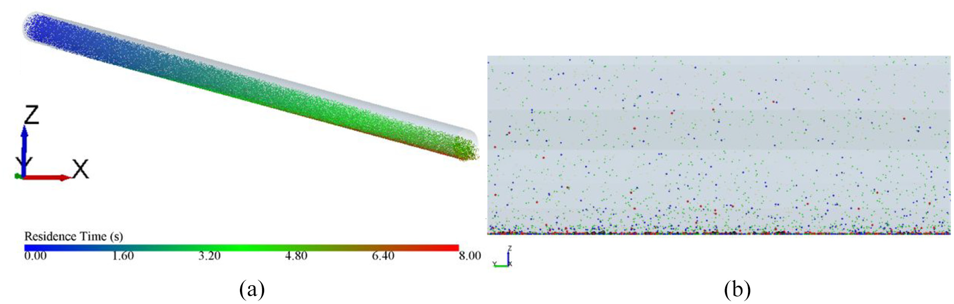
(a) Cloud diagram of particle residence time distribution and (b) distribution law of particles with different diameters.

Figure 8.

Sand concentration in wellbore section at different times.

Figure 7(b) shows the distribution pattern of different particle sizes in the wellbore section, with black representing 590 and 710 μm particles, red representing 500 and 420 μm particles, blue representing 350 and 300 μm particles, green representing 250 and 210 μm particles, yellow representing 177 and 149 μm particles. Small particles approach the upper wall (layer c) with a faster speed, and have a shorter distance and time of movement in the wellbore. The particles are mainly affected by drag force, and the total force is relatively small, so they have better following performance with fluid. As the particle size increases, the velocity decreases, and the distance and time of movement also increase accordingly. Due to the greater influence of inertia force than drag force, the position is biased toward the bottom of the wellbore (layer a).

Figure 8 shows the distribution of sand concentration in the wellbore section at different times, and the sand concentration does not change after stabilization.

Wellbore sand transport model

To quantitatively analyze the law of sand carrying in the wellbore, a geometry model was established with a length of 5 m and an inner diameter of 150.4 mm. The difference in the average volume fraction curve of particles over time with 64,000, 112,000, and 160,000 grids was compared to determine the independence of the grids. Considering computational efficiency and accuracy, 112,000 grids were selected for simulation. In addition to the default convergence criterion, the simulated stability condition is that the variation in the average volume fraction of particles within the calculation domain is less than 10⁻⁴. After stabilization, the sand volume concentration in the wellbore is calculated. The parameters for the sand and fluid are summarized in Table 1, other parameters are the same as section 2, and the particle size distribution is shown in Figure 9.

Table 1.

Parameters of the CFD-DEM coupling simulation.

Viscosity (mPa s)	Velocity (m/s)	Sand production concentration (%)	Well inclination angle (°)	Particle size (μm)
3	0.05	0.005	0	PSD 1
5	0.07	0.01	30	PSD 2
8	0.1	0.03	45	PSD 3
10	0.3	0.05	60	PSD 4
30	0.5	0.1	75
80	1	0.2	90

Figure 9.

Particle size distribution of formation sand.

Calculation method of fractal dimension of formation sand

The results of measuring the PSD of sand particles in a certain formation using a laser particle size analyzer are shown in Figure 10. To evaluate the impact of its particle size distribution on sand carrying in wellbore, the fractal dimension is defined to characterize the formation sand with different particle size distribution.³⁰

Figure 10.

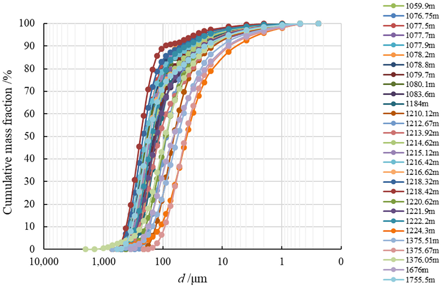
Formation sand size distribution curve.

If the granularity distribution of formation sand has fractal structure, which satisfies with

Y_{n} (x) \propto - x^{- D}

(7)

Where, $Y_{n} (x)$ is total number of particles smaller than diameter x/total number of particles; D is the fractal dimension of the formation sand PSD, dimensionless, and the above formula is written as

d Y_{n} (x) \propto - x^{- 1 - D} dx

(8)

The number of particles $d N$ with diameter between x∼x + dx is expressed as

d N = N d Y_{n} (x)

(9)

Where, N is the total number of particles in the system

Regardless of the difference in particle size and density, the weight of particles $d W$ with size between x∼x + dx is written as

d W = ρ K_{v} x^{3} N d Y_{n} (x)

(10)

Where, $K_{v}$ is the volume shape factor, dimensionless.

Equation (10) can also be written as

d W = W d Y_{W} (x)

(11)

Where, W is the total weight of system particles, kg; $Y_{W} (x)$ is total weight of particles smaller than size/total weight of system particles, kg.

d Y_{W} (x) = ρ N (K_{v} / W) x^{3} d Y_{n} (x)

(12)

Substituting equation (8) into equation (12) yields

d Y_{W} (x) \propto x^{2 - D} dx

(13)

Integrating equation (13) yields

Y_{W} (x) \propto x^{3 - D}

(14)

If the formation sand PSD is satisfied with $Y_{W} (x) \propto x^{b}$ , that is, there is a straight line under the double logarithmic coordinates, which indicates that its particle size distribution has a fractal structure. According to its slope b, the fractal dimension of the particle size distribution can be obtained as: D = 3−b, $Y_{W} (x)$ is the cumulative percentage content of particles with corresponding particle size less than x in the screening curve.

According to the analysis of the measured data of formation sand sample in an oilfield, the formation sand PSD has fractal characteristics. The fractal dimension of formation sand is between 1.95 and 2.45 according to the depth screening analysis data of 11,059.9–1755.5 m in Figure 10. There is a good linear positive correlation between fractal dimension and uniformity coefficient UC, sorting coefficient f, distribution width S. The larger the fractal dimension, the more uneven the particle size distribution is, and the worse the sorting is.

In this paper, different simulation conditions for different sand particle size distributions of formation sand are described with fractal dimension D calculated according to equation (14).

Analysis of factors affecting wellbore cross-section sand concentration and pressure drop

In order to study the sand carrying capacity of the wellbore (the distribution of sand concentration in the cross-section, where position/diameter 0 represents the bottom of the wellbore cross-section and 1 represents the top) and the variation of pressure drop, the effects of different flow rates, viscosities, sand particle size distributions, sand concentration, and wellbore inclination angles were simulated and calculated.

The influence of fluid velocity on cross-section sand concentration and pressure drop

The cross-section velocity and sand volume fraction cloud diagram at 1 m from the inlet (x = 1 m) are shown in Figure 11(a) and (b) under three flow velocity 0.05, 0.3, and 1 m/s, with the same other parameters: particle size PSD1, well inclination angle 60°, viscosity 30 mPa s, and concentration 0.03%. The fluid velocity gradually increases radially from the lower pipe wall, and gradually decreases after reaching the maximum value in the middle part. The sand concentration is symmetrically distributed on both sides of the wellbore.

Figure 11.

(a) Fluid velocity cloud diagram in cross section (x = 1 m), (b) cloud diagram of sand volume fraction in cross section of horizontal wellbore with different fluid velocity, (c) distribution curve of sand volume fraction in cross section of horizontal wellbore with different flow velocity, and (d) relationship curve between wellbore axis pressure drop and flow velocity.

The cross-section sand concentration of the wellbore is significantly stratified under different flow velocity conditions, as shown in Figure 11(c) (where a position/pipe diameter of 0 represents the bottom of the wellbore cross-section and 1 represents the top). Since particle velocities are all greater than 0, the concentration in areas with a deposition concentration ratio greater than 1 has not yet reached the fixed bed concentration. Therefore, the flow in the wellbore is divided into heterogeneous suspended layers and suspended layers. The sand content in the suspended layer tends to stabilize at 0.2–1 time of the pipe diameter, with a small gradient change, and the maximum sand content is below 0.1%. The maximum sand mass fraction of the heterogeneous suspended layer is 20 times the sand production concentration, with a significant gradient variation. The larger the flow velocity is, the closer the pipe diameter position to the bottom of the wellbore cross-section is where the volume fraction of sand in the heterogeneous suspended layer significantly increases.

The sand concentration in the suspended layer increases, while the sand concentration in the heterogeneous suspended layer decreases with the increase of fluid velocity, and the height change is relatively stable. From this, the main controlling factor affecting the sand carrying capacity of the wellbore is the sand concentration in the suspended layer, that is, the higher the fluid velocity is, the higher the sand concentration in the suspended layer, and the stronger the sand carrying capacity is.

Due to the presence of fluid hydrostatic pressure under gravity, the pressure difference between the inlet and outlet of a vertical wellbore is inevitably much greater than that of a horizontal wellbore. Therefore, the unit length pressure drops after excluding the static pressure generated by gravity is used to study the pressure loss inside the wellbore with the existence of sand particles. From Figure 11(d), the pressure drop along the wellbore axis increases approximately linearly with the increase of flow velocity, and the influence of different well inclination angles on the pressure drop is not significant.

The influence of fluid viscosity on cross-section sand concentration and pressure drop

The cross-section sand volume fraction cloud diagram and curve graph at 1m from the inlet (x = 1 m) are shown in Figure 12(a) and (b) under three flow viscosity 3, 30, and 80 mPa s, with the same other parameters: particle size PSD1, well inclination angle 60°, velocity 0.5 m/s, and concentration 0.03%. The sand volume fraction in the suspended layer gradually increases with the increase of fluid viscosity, while the sand volume fraction in the heterogeneous suspended layer gradually decreases, enhancing the fluid’s ability to carry sand. At the same time, as the fluid viscosity increases, the sand content in the suspended layer near the top of the wellbore first increases and then tends to stabilize. The larger the viscosity is, the more obvious this change is. The sand content in the top is close to 0 with 3 mPa s, indicating that the fluid viscosity has a significant impact on the sand content in both the heterogeneous suspended layer and the suspended layer. From Figure 12(c), the pressure drop along the wellbore axis increases linearly with the increase of fluid viscosity, and the effect of different well inclination angles on the pressure drop is not significant.

Figure 12.

(a) Cloud diagram of sand volume fraction in cross section of horizontal wellbore with different fluid viscosity, (b) distribution curve of sand volume fraction in cross section of horizontal wellbore with different viscosity, and (c) relationship curve between wellbore axial pressure drop and fluid viscosity.

The influence of sand particle size distribution on cross-section sand concentration and pressure drop

The cross-section sand volume fraction cloud diagram and curve graph at 1m from the inlet (x = 1 m) are shown in Figure 13(a) and (b) under three PSDs, PSD1, PSD2, and PSD4, with the same other parameters: viscosity 30 mPa s, well inclination angle 60°, velocity 0.5 m/s, and concentration 0.03%. As the effective particle size increases, the volume fraction of the solid phase in the suspended layer decreases when the flow is stable. The volume fraction of the sand in the heterogeneous suspended layer increases, and the sand carrying capacity of the fluid decreases. The larger the effective particle size is, the more stable the distribution of the sand volume fraction at the top of the suspended layer is. Meanwhile, as shown in Figure 13(c), the pressure drop along the wellbore axis does not change significantly with the increase of the effective particle size of the sand particles. The variation range of pressure drop under different PSD is between 5.7296 and 50.4111 Pa. When the effective particle size is the same, the fluid velocity has a significant impact on the pressure drop in the horizontal wellbore, with a maximum of 1455.14 Pa.

Figure 13.

(a) Cloud diagram of particle volume fraction in cross section of horizontal wellbore with different sand particle size distribution, (b) distribution curve of sand volume fraction in cross section of horizontal wellbore with different particle sizes, and (c) relationship curve between wellbore axial pressure drop and different sand particle sizes.

The influence of sand production concentration on cross-section sand concentration and pressure drop

The cross-section sand volume fraction cloud diagram and curve graph at 1 m from the inlet (x = 1 m) are shown in Figure 14(a) and (b) under three sand concentration, 0.005%, c = 0.03% and c = 0.2%, with the same other parameters: viscosity 30 mPa s, well inclination angle 60°, velocity 0.5 m/s, and concentration 0.03%, PSD1. The higher the sand concentration is, the higher the sand content in both the heterogeneous suspended layer and the suspended layer is. The height of the heterogeneous suspension layer remains basically unchanged and remains between 0.2 times the pipe diameter. Meanwhile, as shown in Figure 14(c), with the increase of sand concentration, the pressure drop along the horizontal wellbore axis increases, and the pressure drop varies between 230.6 and 484.86 Pa under different concentration and the same particle size distribution conditions. Under the same sand concentration and different particle size distribution conditions, the pressure drop changes significantly, ranging from 93.82 to 334.13 Pa.

Figure 14.

(a) Cloud diagram of particle volume fraction in cross section of horizontal wellbore with different sand production concentration, (b) distribution curve of sand volume fraction in horizontal wellbore section with different sand production concentration, and (c) relationship curve between wellbore axial pressure drop and different sand production concentration.

The influence of well inclination angle on cross-section sand concentration and pressure drop

The cross-section sand volume fraction cloud diagram and curve graph at 1 m from the inlet (x = 1 m) are shown in Figure 15(a) and (b) under three well inclination angles, 30°, 60°, and 90°, with the same other parameters: viscosity 30 mPa s, velocity 0.5 m/s, and concentration 0.03%, PSD1. When the inclination angle of the well increases, the volume fraction of sand in the heterogeneous suspended layer increases, but the height remains between 0.25 times the pipe diameter, and the volume fraction of sand in the suspended layer decreases. When the inclination angle of the well is 0°, the volume fraction of sand in the cross-section is symmetrically distributed. At the same time, as shown in Figure 15(c), as the inclination angle increases, the pressure drop along the wellbore axis gradually decreases. The higher the sand concentration with the same inclination angle of the well is, the greater the pressure drop is.

Figure 15.

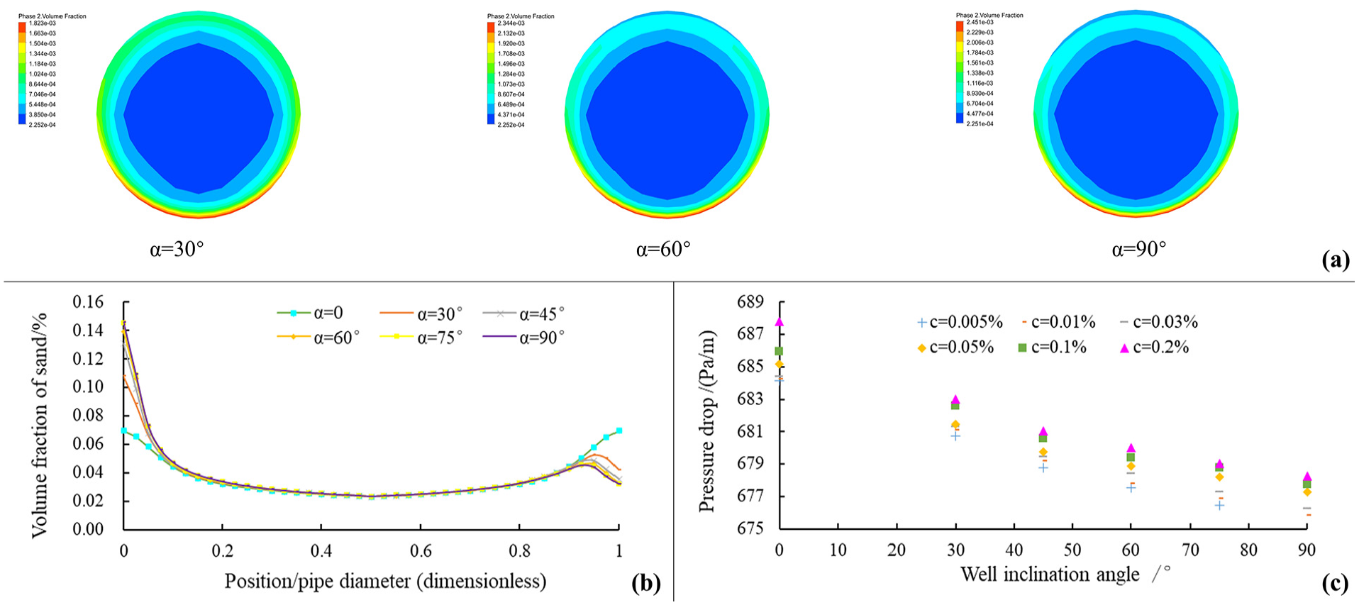
(a) Cloud diagram of particle volume fraction in cross section of horizontal wellbore with different well deviation angles, (b) distribution curve of sand volume fraction in horizontal wellbore section with different well deviation angles, and (c) relationship curve between wellbore axis pressure drop and different well deviation angles.

Prediction model for critical non-deposition flow velocity and wellbore sand volume concentration

Critical non-deposition flow velocity

The influence of effective sand particle size, sand production concentration, and fluid viscosity on the volume concentration of sand particles in horizontal wellbore under different flow velocity conditions is shown in Figure 16. Over 100 sets of simulated data are obtained in total.

Figure 16.

(a) Influence of flow velocity on sand volume fraction with PSD1, 0.03%, 3 mPa s, (b) influence of flow velocity on sand volume fraction with PSD1, 0.03%, 10 mPa s, (c) influence of flow velocity on sand volume fraction with PSD1, 0.03%, 30 mPa s, (d) influence of flow velocity on sand volume fraction with PSD2, 0.03%, 30 mPa s, (e) influence of flow velocity on sand volume fraction with PSD4, 0.03%, 30 mPa s, (f) influence of flow velocity on sand volume fraction with PSD1, 0.005%, 30 mPa s, and (g) influence of flow velocity on sand volume fraction with PSD1, 0.2%, 30 mPa s.

It can be seen that the shape of the curve conforms to the widely used Pareto’s law in social statistics. The principle is that 20% of the independent variables are within the range of qualitative change and have a decisive effect on things. A small change in the independent variables will cause a sharp change in the dependent variable; Another 80% are in the process of accumulating quantitative changes, and large changes in the independent variable are also difficult to cause fluctuations in the dependent variable, presenting an overall power-law distribution type. The power-law distribution represents a process of transitioning from a steady state to a chaotic state, where there must exist a critical value. When the flow rate is high, the concentration of sand particles in the wellbore is close to the sand production concentration 0.03%, indicating that there is almost no sand settling in the wellbore and the curve changes smoothly. As the flow rate gradually decreases, the concentration of sand particles in the wellbore gradually increases. When the flow rate decreases to a certain extent, a small decrease in flow rate will cause a sharp increase in the concentration of sand particles, with an exponential growth trend. Therefore, the curve variation can be roughly divided into three parts: the stable zone, the growth zone, and the transition zone where the two intersect. The critical non- deposition velocity is located in the transition zone where two changing trends intersect. There is a critical point in the transition zone, where the absolute slope value of any point on the curve before the critical point rapidly decreases with the increase of flow velocity, while the change behind the critical point is not significant. The corresponding flow velocity at this point is the critical non-deposition flow velocity. The determination method is to use linear fitting for the flat zone and exponential growth zone, where the intersection point of the fitting straight line represents the turning point of the two changing trends. The flow velocity corresponding to the abscissa of this point is the critical non-deposition flow velocity under this condition. Its engineering significance is that when the flow velocity is less than this value, a small change causes a rapid sand concentration increase in the in the wellbore, resulting in a corresponding increase in the amount of sand settling. The critical non-deposition flow velocity under different flow conditions is shown at the intersection of the curves in Figure 16.

The changes in critical non-deposition flow velocity with fluid viscosity, formation sand production concentration, and effective particle size are shown in Figure 17, respectively. As the particle size increases, gravity plays a dominant role, and the critical non-deposition velocity of sand particles gradually decreases with the increase of fluid viscosity, and increases with the increase of formation sand production concentration and effective particle size.

Figure 17.

(a) Critical velocity with different fluid viscosity, (b) critical velocity with different sand production concentration, and (c) critical velocity with different formation sand effective particle size.

Prediction model of wellbore sand volume concentration based on fractal dimension of formation sand

The concentration of sand particles is a key parameter for sand carrying in the wellbore. After analyzing the simulated data in section “Critical non-deposition flow velocity,” the concentration of sand particles in the horizontal wellbore $C_{w}$ is a function of the formation sand production concentration C_s, fluid flow velocity $ν$ , fluid density $ρ$ , fluid viscosity $μ$ , effective sand particle size $d 50 / D$ , and wellbore diameter $D_{w}$ , which can be expressed by the following equation

f_{2} (C_{w}, C_{s}, d 50, ν, D, ρ, μ, D_{w}) = 0

(15)

Apply Buckingham-Π to the above variables and define four dimensionless quantities with practical significance, namely the dependent variable horizontal wellbore sand particle concentration ( $π_{c 1}$ , $C_{w}$ ), the independent variable formation sand production concentration ( $π_{c 2}$ , $C_{s}$ ), the dimensionless quantity representing the effect of effective particle size on sand carrying( $π_{c 3}$ , $d 50 / (D * D_{w})$ ), and the dimensionless quantity representing the Reynolds number of wellbore circular pipes ( $π_{c 4}$ , $\frac{ρ ν D_{w}}{μ}$ ). The direct relationship between the four dimensionless quantities is described by the following equation

C_{w} = π_{c 1} = f_{2} (π_{c 2}, π_{c 3}, π_{c 4})

(16)

Through nonlinear fitting analysis, the equation form is as follows

C_{w} = π_{c 1} = B \cdot π_{c_{2}}^{a_{2}} \cdot π_{c_{3}}^{a_{3}} \cdot π_{c_{4}}^{a_{4}}

(17)

Where, B, a₂, a₃, a₄ is coefficient.

According to the variation of the volume concentration of sand particles $C_{w}$ with various influencing factors, the model coefficients were obtained through data fitting, as shown in Table 2.

Table 2.

Fitting results and coefficients for the proposed model.

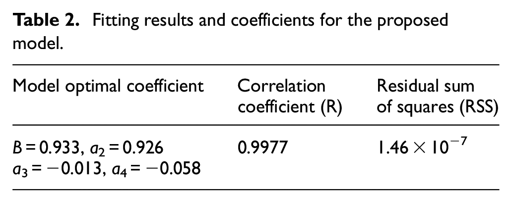
Model optimal coefficient	Correlation coefficient (R)	Residual sum of squares (RSS)
B = 0.933, a₂ = 0.926 a₃ = −0.013, a₄ = −0.058	0.9977	1.46 × 10⁻⁷

The prediction equation for sand volume concentration is

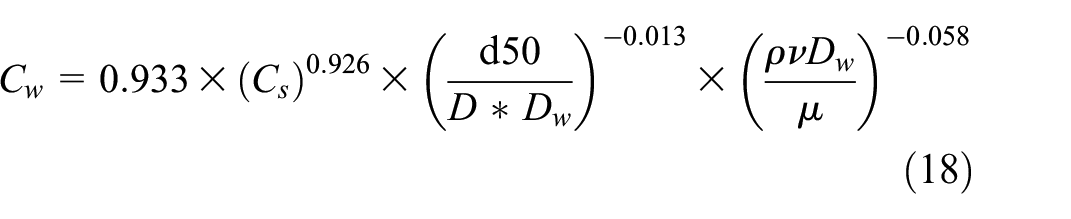
C_{w} = 0.933 \times {(C_{s})}^{0.926} \times {(\frac{d 50}{D * D_{w}})}^{- 0.013} \times {(\frac{ρ ν D_{w}}{μ})}^{- 0.058}

(18)

The comparison between the simulated and predicted values of sand volume concentration is shown in Figure 18. The correlation coefficient of the fitting results is 0.9977, which can accurately predict the volume concentration of sand particles in the wellbore within the assumed conditions.

Figure 18.

Comparison between simulated value and predicted value of wellbore sand volume concentration.

Conclusions

In this paper, a coupled CFD–DEM approach has been presented to simulate the effects of the well inclination, sand size distribution, fluid viscosity, sand production concentration, and fluid inlet velocity on the sand carrying process. It provides a more realistic modeling of discrete suspended particles through coupled DEM.

The influence of sand particle size distribution, fluid velocity, viscosity, sand production concentration, well inclination angle on the cross-section sand concentration, and wellbore axis pressure drop was analyzed. The main controlling factor affecting the sand carrying capacity of the wellbore is the sand concentration of the suspended layer. The pressure drop along the wellbore axis increases approximately linearly with the increase of flow velocity and fluid viscosity.

Method for determining the critical non-deposition flow of sand particles transportation in the wellbore is proposed. Based on the influence of fluid velocity on the concentration of sand in the wellbore, a linear fitting of the gentle and exponential growth regions of the sand volume fraction and concentration curve is used. The intersection of the fitted straight lines represents the turning point of the two changing trends. The flow velocity corresponding to the abscissa of this point is defined as the critical non-deposition flow velocity under this condition.

Considering the distribution of formation sand particle size, a dimensional analysis method was used to establish a prediction model for the volume concentration of sand particles in the horizontal well section, which is convenient for engineering applications to quickly determine the flow status of the wellbore.

Footnotes

Acknowledgements

The author thanks the institution for allowing the publication of this research paper.

Handling Editor: Sharmili Pandian

Author contribution

Liu Shanshan: Conceptualization; Methodology; Investigation; Formal analysis; Writing – original draft; Project; Writing – review & editing.

Declaration of conflicting interests

The author declared no potential conflicts of interest with respect to the research, authorship, and/or publication of this article.

Funding

The author received no financial support for the research, authorship, and/or publication of this article.

ORCID iD

Liu Shanshan

References

Walton

Atwood

Halleck

, et al. Perforating unconsolidated sands: an experimental and theoretical investigation. In: SPE annual technical conference and exhibition, New Orleans, LA, USA, September 2001.

Van den Hoek

Hertogh

GMM

Kooijman

, et al. A new concept of sand production prediction: theory and laboratory experiments. SPE Drill Completion 2000; 15: 261–273.

Liu

Wang

. Formation grain size profile prediction model considering the longitudinal continuity of reservoir using artificial intelligence tools. In: SPE/IATMI Asia Pacific oil & gas conference and exhibition, Virtual, 12–14 October 2021, paper no. SPE-205683-MS.

Liu

Zhao

Wang

Artificial intelligence method for shear wave travel time prediction considering reservoir geological continuity. Math Probl Eng 2021; 2021: 5520428.

Liu

A grain size profile prediction method based on combined model of extreme gradient boosting and artificial neural network and its application in sand control design. SPE J 2024; 29: 2988–3002.

Zhou

Choi

SK.

Numerical simulation of the liquid-induced erosion in a weakly bonded sand assembly. Powder Technol 2011; 211: 237–249.

Younessi

Khaksar

Hogue

, et al. Sand production prediction analyses at different stages of geographe field development. In: SPE Asia Pacific oil & gas conference and exhibition, Adelaide, SA, Australia, 17–19 October 2022.

Tao

Chen

Liu

Application and practice of integrated sand control technology in shallow heavy oil reservoirs in Kazakhstan. In: SPE annual Caspian technical conference, Nur-Sultan, Kazakhstan, 15–17 November 2022.

Bai

Zhou

, et al. Experimental study on type and accuracy optimization of sand control in sand-producing heavy oil well. In: SPE Eastern Europe subsurface conference, Kyiv, Ukraine, 23–24 November 2021.

10.

Eltaher

Nasser

Tarihoran

, et al. Trial and assessment of a new downhole sand production measurement in oil and gas wells. In: SPE reservoir characterisation and simulation conference and exhibition, Abu Dhabi, UAE, 24–26 January 2023.

11.

Bianco

LCB

Halleck

. Mechanisms of arch instability and sand production in two-phase saturated poorly consolidated sandstone. In: SPE European formation damage conference, The Hague, Netherlands, 21–22 May 2001.

12.

Mondal

Sharma

Chanpura

, et al. Numerical simulations of sand-screen performance in standalone applications. SPE Drill Completion 2011; 26: 472–483.

13.

Baldini

Carlevaro

Pugnaloni

, et al. Numerical simulation of proppant transport in a planar fracture. A study of perforation placement and injection strategy. Int J Multiph Flow 2018; 109: 207–218.

14.

Lezhnev

. Application of discrete element method for modelling sand control systems. In: SPE Russian petroleum technology conference, Moscow, Russia, 15–17 October 2018.

15.

Ghassemi

Pak

Numerical simulation of sand production experiment using a coupled Lattice Boltzmann-Discrete Element Method. J Pet Sci Eng 2015; 135: 218–231.

16.

Alaita

Hossain

Islam

SZ.

Modelling multiphase flow in vertical pipe using CFD method. In: Abdel Wahab

(ed.) International conference on numerical modelling in engineering. Singapore: Springer, 2019, pp.300–319.

17.

Yan

Sun

, et al. Numerical investigation on horizontal wellbore hole cleaning with a four-lobed drill pipe using CFD-DEM method. Powder Technol 2020; 375: 249–261.

18.

Dabirian

Mohan

Shoham

, et al. Sand flow regimes in slightly upward inclined gas-liquid stratified flow. In: American Society of Mechanical Engineers, fluids engineering division summer meeting, Washington, DC, USA, 10–14 July 2016.

19.

Dabirian

Mohan

Shoham

, et al. Solid-particles flow regimes in air-water stratified flow in a horizontal pipeline. Oil Gas Facil 2016; 15: 1–14.

20.

Durand

Basic relationships of the transportation of solids in pipes-experimental research. In: Proceedings of the international association of hydraulic research, Minneapolis, MN, USA, 1–4 September 1953, pp.89–103. Minneapolis: Minnesota.

21.

Oroskar

Turian

RM.

The critical velocity in pipeline flow of slurries. AIChE J 1980; 26: 550–558.

22.

Davies

JT.

Calculation of critical velocities to maintain solids in suspension in horizontal pipes. Chem Eng Sci 1987; 42: 1667–1670.

23.

Najmi

McLaury

Shirazi

, et al. The effect of viscosity on low concentration particle transport in single-phase (liquid) horizontal pipes. J Energy Resour Technol 2016; 138: 032902.

24.

Soepyan

Cremaschi

Sarica

, et al. Solids transport models comparison and fine-tuning for horizontal, low concentration flow in single-phase carrier fluid. AIChE J 2014; 60: 76–122.

25.

Wicks

Transport of solids at low concentration in horizontal pipes. In: Zandi

(ed.) Advances in solid-liquid flows in pipes and its application. Oxford: Pergamon Press, 1971, pp.101–124.

26.

Holt

RM.

Particle scale reservoir mechanics. Oil Gas Sci Technol 2002; 57: 525–538.

27.

Tallak

Rothenburg

Dusseault

Hydraulic fracture (parting) simulation in granular assemblies using the discrete element method. AOSTRA J Res 1990; 6: 141–153.

28.

Potyondy

Cundall

PA.

A bonded-particle model for rock. Int J Rock Mech Min Sci 2004; 41: 1329–1364.

29.

Long

, et al. The mechanism of emitter clogging analyzed by CFD-DEM simulation and PTV experiment. Adv Mech Eng 2018; 10: 168–192.

30.

Mandelbrot

BB.

The fractal geometry of nature. Am J Phys 1983; 51: 286.

Study on factors influencing sand migration in wellbores