Sage Journals: Discover world-class research

Abstract

This study predicted the performance of an inlet guide vane to be installed later by applying an absolute flow angle (ß) at the axial pump inlet. The pump’s performance was predicted based on changes in inlet ß, and the influence of variations in inlet ß on the low-flow area was analyzed. For turbulence flow analyses, the Reynolds-averaged Navier–Stokes equations were discretized based on the finite volume method. The internal flow was analyzed in detail through transient analysis. Furthermore, the impact of changes in the absolute flow angle at the inlet on the rotating stall occurring inside the pump in the low-flow-rate region was analyzed. The analysis of the internal flow field confirmed that the absolute flow angle at the inlet affects the stability of the internal flow. Results showed that energy reduction and efficient operation scenarios can be established compared with the existing valve control method by changing inlet ß. Through fast Fourier-transform analysis, it was confirmed that when the inlet angle (θ) is changed in the low-flow-rate region, a more stable operation is possible compared with the existing one.

Keywords

Axial-flow pump inlet guide vane inlet flow angle surging rotating stall hydrodynamic performance energy saving

Introduction

Fluid machinery are devices that convert the energy contained in viscous and compressible fluids (e.g. water and air) into mechanical energy. Pumps are a type of fluid machinery that imparts energy to water to increase pressure or convey it to a higher elevation. Pumps can be further classified as centrifugal, mixed-flow, and axial-flow types. Axial-flow pumps have a high specific speed that makes them suitable for applications involving a relatively low head but high flow rates, such as in agriculture, sewage systems, and storm-water drainage channels. The impeller is a core component of the axial-flow pump that increases the velocity and pressure of the fluid through the lift of its blades and causes the fluid to flow from the inlet to the outlet. Thus, many studies have focused on enhancing the axial-flow pump performance by optimizing the shape, angle, and installation position of the impeller.^1–3 At low flow rates, the hydraulic performance of axial-flow pumps is unstable compared to centrifugal pumps due to the surging phenomenon. This is because the saddle region occurs at low flow rates, where the flow and pressure vary periodically. Thus, operating axial-flow pumps at low flow rates should generally be avoided.

The variable inlet guide vane (IGV) is an axial-flow pump component that is typically installed near the leading edge of the impeller and that influences the flow angle. In the event of a load change, the IGV can be adjusted to change the flow angle in response. Kaya⁴ conducted experiments to analyze the effect of installing an IGV in an axial-flow pump and confirmed that it improved the pump performance. They also analyzed the influence of the IGV thickness on the pump performance. Ahmed et al.⁵ and Junaidi et al.⁶ numerically analyzed the effect of installing an IGV on the pump efficiency and internal flow to determine the optimal installation location. Hu et al.⁷ analyzed the changes in internal flow and performance according to the installation location of the IGV. Tang and Wang⁸ optimized the internal hydraulic performance of a pump according to the IGV installation location and blade thickness and reported a performance improvement of about 10%. Qian et al.⁹ conducted experiments to analyze the effect of the IGV on the pump performance in the off-design point state and confirmed that optimizing the flow angle improved the pump efficiency by up to 2.16% and reduced the range of unstable operation. Chan et al.¹⁰ numerically analyzed the effect of the IGV on the vortex at the leading edge of the impeller and optimized the flow angle to improve the pump performance. Xu et al.¹¹ conducted numerical analyses and experiments to evaluate the changes in pump performance at the same flow point based on the IGV. Li and Wang¹² and Li et al.¹³ conducted numerical analyses and experiments to evaluate changes in the internal flow characteristics and hydraulic performance when an IGV is installed inside an axial-flow pump. They confirmed that the IGV changes the flow angle, which affects the angle of incidence and in turn the pump performance. Installing an IGV inside the pump allows the flow angle to be adjusted for improved efficiency, reduced shaft power consumption, and increased operational range of flow rates.^14,15 Many studies have focused on using the IGV to change the flow angle and improve the pump performance.^16–18 Choi et al.¹⁹ analyzed operational scenarios to determine the optimal setup. Zierke et al.²⁰ numerically analyzed the three-dimensional turbulence flow of an axial-flow pump equipped with an IGV and compared their findings with experimental results. They analyzed the internal flow phenomena of the pump and the characteristics of the IGV, and they constructed a database to facilitate smooth pump operation. Feng et al.²¹ conducted experiments to analyze the change in characteristics of an axial-flow pump according to the tip clearance of the IGV. Liu et al.²² analyzed the internal flow distribution of an axial-flow pump according to the installation position of the IGV to determine the optimal flow angle. Kim and Kim²³ analyzed the effect of the IGV thickness on the internal flow and performance characteristics of an axial-flow pump. Watanabe et al.²⁴ conducted experiments to analyze the performance characteristics of an axial-flow pump at low flow rates as well as the effects of a surging phenomenon. Qian et al.²⁵ analyzed the changes in the internal flow field, total head, and efficiency of a pump according to the flow angle. They installed an IGV on a pump turbine of a hydroelectric power plant and developed an efficient operating plan. Tan et al.^26,27 compared the performances of IGVs designed in three dimensions (3D) and two dimensions (2D). They confirmed that the 3D design method produced an IGV that was 2.13% more efficient. Research is actively ongoing on the effects of installing an IGV as well as the angle and shape of its blades on the hydraulic performance of the axial-flow pump.^28,29

Most of the above studies actually installed an IGV inside a pump to evaluate its effects. However, the approach of installing an IGV and then modifying its design to identify optimal operational scenarios at low flow rates is impractical in terms of both cost and time. In this study, a swirling flow was artificially applied at the trailing edge of the IGV, and the flow angle at the inlet of the pump was set. Numerical analyses were performed to predict the pump performance and analyze unstable flow phenomena at low flow rates. This approach allows the effect of the IGV on the hydraulic performance of an axial-flow pump at low flow rates to be predicted before its actual installation.

Methods

Pump model

In this study, a 3D model of an axial-flow pump comprising a de-swirler (DS), an impeller, and a diffuser vane (DV) was employed, as shown in Figure 1. The DS blocks impurities that may be introduced by the impeller. The impeller increases the velocity and pressure of the fluid while the DV slows it down. The design specifications are presented in Table 1. The specific speed N_s was calculated as follows:

N_{s} = \frac{ω \sqrt{Q}}{{(gH)}^{3 / 4}}

(1)

where $ω$ , Q, g, and H are the angular velocity (rad/s), flow rate (m³/s), gravitational acceleration (m/s²), and total head (m), respectively. The nondimensional flow coefficient $Φ$ , total head coefficient $Ψ$ , and shaft power coefficient $λ$ were calculated as follows:

Φ = \frac{c_{m 2}}{u_{2}}

(2)

Ψ = \frac{2 gH}{u_{2}^{2}}

(3)

λ = \frac{L}{\frac{1}{2} ρ A_{2} {u_{2}}^{3}}

(4)

where $C_{m 2}$ is the meridional component of the absolute velocity at the impeller outlet (m/s), $u_{2}$ is the rotational velocity at the impeller outlet (m/s), L is the shaft power (W), $ρ$ is the density (kg/m³), and A is the area (m²).

Figure 1.

Computational domain of the pump model.

Table 1.

Design specifications of the pump model.

Description	Value
Specific speed ( $N_{s}$ )	2.94
Flow coefficient ( $Φ)$	0.249
Head coefficient $(Ψ)$	0.239
Shaft power coefficient $(λ)$	0.079
Rotational speed (rpm)	2560
Impeller diameter (mm)	185
Number of de-swirlers	4
Number of impeller blades	4
Number of diffuser vanes	7

Artificial application of an IGV

Installing an IGV in an axial-flow pump changes the inlet flow angle θ, which is the angle of incidence of the flow into the impeller. Changing θ affects the hydraulic performance of the pump, and changes in load can be managed by changing θ. In this study, the absolute flow angle β was used to represent the IGV in the design phase. Absolute flow angles (β) of 0°, 25°, and 45° were utilized based on the direction of the impeller rotation. Numerical analyses were performed to evaluate the hydraulic performance of the pump at different β, which could be used to predict the effectiveness of the IGV in different operational scenarios, including load changes and low flow rates. Figure 2 shows the velocity triangles at the impeller inlet and shroud span at β = 0°, 25°, and 45° where w, u, and c are the relative velocity, tangential velocity, and absolute velocity, respectively. The solid black arrows indicate the operating conditions without the IGV while the red dashed arrows indicate the operating conditions with the IGV. Through the schematic of the velocity triangle, it can be predicted that, for the same mass flow rate and rotational speed conditions, different absolute flow angles at the inlet cause changes in the incidence angle of the flow entering the impeller. Figure 2 shows that the use of different flow angles at the inlet changes the incidence angle of the flow entering the span of the impeller shroud. The value of β was determined with respect to the axial direction at the inlet of the pump domain. Changing β affects H and the normalized total efficiency (η) owing to changes in Ф and θ corresponding to the best efficiency point (BEP), which in turn changes the performance characteristics.

Figure 2.

Velocity triangles at the impeller inlet (left) and shroud span (right) at different absolute flow angles β with (red dashed arrows) and without (solid black lines) the IGV.

Numerical analysis

Figure 3 shows the model used for numerical analyses. Figure 3(a) shows the reference model, which comprised an inlet with the shape of a bell mouth, a DS, an impeller, a DV, and an outlet. The IGV is likely to be installed at the location of the DS. Furthermore, β imposed at the inlet may be influenced by the DS as the flow progresses. Figure 3(b) shows the simplified model, which simplifies the inlet by removing the DS. Both models share the same axial length. To facilitate smooth convergence during the numerical analysis, the lengths of the inlet and outlet sections were expanded to 3.5 times the diameter.

Figure 3.

3D model comparison: (a) reference model and (b) simplified model.

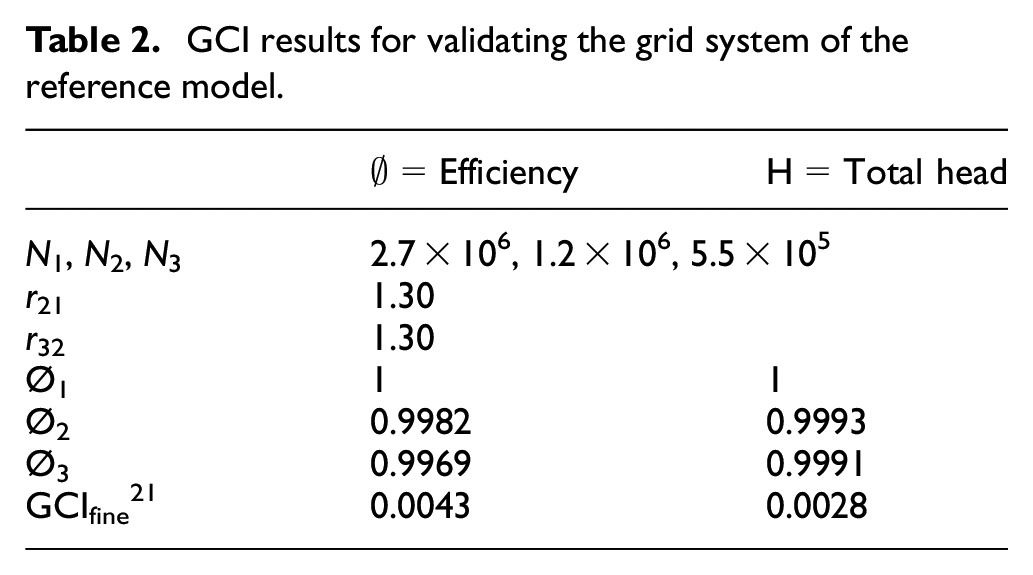
Figure 4 shows the grid employed in this study, which comprised a hexahedral mesh. A grid evaluation test was performed using the grid convergence index (GCI) method proposed by Celik et al.,³⁰ and the results are presented in Figure 5 and Table 2. To validate the grid system, three different grids were constructed, and numerical analysis was performed at the design flow point to compare H and total efficiency Ø, which in turn was normalized with respect to the results of the finest grid (i.e. N₁) to obtain η. N₁ had GCIs of approximately 0.0043 and 0.0028, which satisfied the convergence criterion proposed by Celik et al.³⁰ Therefore, N₁ was applied as the grid.

Figure 4.

Model and grid used for numerical analyses.

Figure 5.

GCI results using the grid system of the reference model.

Table 2.

GCI results for validating the grid system of the reference model.

	$\emptyset = Efficiency$	$H = Total head$
N ₁, N₂, N₃	2.7 × 10⁶, 1.2 × 10⁶, 5.5 × 10⁵
r ₂₁	1.30
r ₃₂	1.30
Ø₁	1	1
Ø₂	0.9982	0.9993
Ø₃	0.9969	0.9991
GCI_fine²¹	0.0043	0.0028

Numerical analyses were performed by using the computational fluid dynamics analysis (CFD) program CFD-19.2.³¹ The turbulence of the flow was analyzed by using Reynolds-averaged Navier–Stokes (RANS) equations discretized according to the finite volume method.³² Time-dependent terms were added to each governing equation for transient analysis. The shear–stress transport (SST) turbulence model was employed to accurately identify flow separation.³³ With regard to convergence, imposing the pressure and mass flow rate at the inlet and outlet would be advantageous. However, in this study, β at the inlet had to be given, so the flow distribution at the inlet had to be uniform. Therefore, the mass flow rate and atmospheric pressure conditions were set at the inlet and outlet. To enhance convergence, periodic conditions were applied to the rotating direction of one blade passage. A frozen rotor was implemented between the stator and stator, and a stage-averaged technique was applied between the rotor and stator. The operating fluid was water at 25°C. For transient analysis, the time corresponding to one rotation of the pump was 0.023 s, and data were collected every 3° for detailed information. Numerical analyses were performed by using a 32-core dual-processor Xeon (2.8 GHz) central processing unit. The processing time to analyze the steady state of one blade passage was about 5 h, and the processing times to analyze the steady and transient states of all blade passages were about 11 h and 10 days, respectively.

Model validation

The experiments on the investigated axial-flow pump were performed at the Korea Institute of Industrial Technology (KITECH). Figure 6 shows a schematic of the test equipment used in evaluating the performance of the axial-flow pump, along with measurement devices. The experiments were performed in a closed-loop test system equipped with a variable-angle IGV, an impeller, and diffuser vanes. As shown in the diagram, the test equipment and measurement devices included the axial-flow pump, a butterfly valve, a power meter, a tachometer, pressure sensors, and an electronic flow meter. The scope of the test and precision of measurements and instruments satisfied the requirements of the KS B6301 standard. For performance evaluation, performance curves were obtained, including design flow points and off-design points, at IGV angles of 0°, 25°, and 45°.

Figure 6.

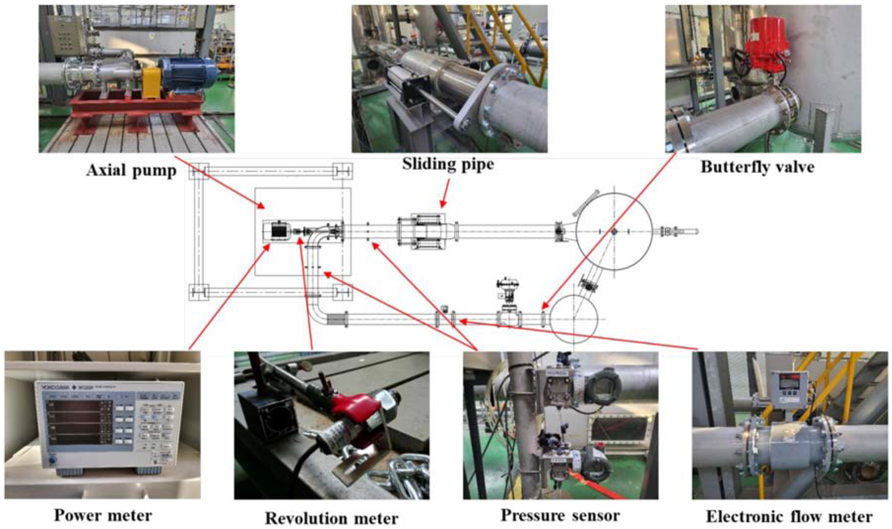
Schematic of the axial-flow pump testing facility and measuring devices.

Figure 7 shows the performance curves for the numerical analyses of the reference and simplified models and an experiment using the reference model. Overall, the experimental and numerical results of the reference model demonstrated consistency and similarity. Both models showed inflection points at Ф = 0.10 and 0.21 and predicted similar performances at the design flow coefficient Ф_d and high flow rates. However, differences in the predicted performance were observed below the saddle region, especially at Ф < 0.2. This implies that the DS influences the performance at low flow rates. These phenomena were induced as β increased. Kim et al.³⁴ previously showed that the presence of an anti-stall fin with a form similar to the DS at the inlet of turbomachinery greatly influences the internal flow stability. The DS helps prevent unstable flow phenomena with the pump. The performance curve of the simplified model shown in Figure 3(b) was obtained without the DS. At low flow rates, the predicted performance exhibited a slight decrease. However, this region was not considered part of the operational range of the pump. At Ф > 0.21, the simplified model generally exhibited similar trends as the reference model. The results shown in Figure 7 have already been verified in previous studies.^35,36 The above results indicated that the simplified model could be used for analysis without any major issues.

Figure 7.

Comparison of CFD and experimental results.

Results

Hydraulic performance

Figure 8 shows the hydraulic performance curves of the simplified model at different β for the (a) total head coefficient Ψ, (b) normalized total efficiency η, and (c) shaft power coefficient λ. As shown in Figure 8(a), increasing β to 25° and 45° caused Ψ to decrease, which indicates that the operational range of the pump was reduced. With β = 0°, the performance curve showed a positive slope at the flow coefficient Ф ≤ 0.2. The positive slope disappeared at β = 25° and 45°. At low Ф, a saddle zone was observed where the flow rate and pressure were unstable. The surging phenomenon generates noise and vibration inside the pump, which affects its durability and performance. At β = 0°, the change in the positive slope was remarkable at low Ф. The deepest inflection point was observed at Ф = 0.106, and the positive slope disappeared at Ф > 0.2. The positive slope decreased as β increased, and the positive slope could not be observed at β = 45°. As shown in Figure 8(b), increasing β caused Ф corresponding to the BEP decreased, and the absolute value of η corresponding to the BEP also decreased.

Figure 8.

Hydraulic performance curves at different absolute flow angles β for the (a) total head coefficient Ψ, (b) normalized total efficiency η, and (c) shaft power coefficient λ.

With the existing valve control method, the pump cannot operate at low flow rates owing to the surging phenomenon that causes unstable operation. The above results indicate that installing an IGV (i.e. increasing β) eliminates the positive slope that causes unstable flow, which will allow the pump to operate even at low flow rates. However, it is difficult to judge whether the unstable flow has been completely resolved. Therefore, the internal flow field was analyzed to clarify the flow phenomena at low flow rates with varying β.

Axial-flow pumps are often used at sites with frequent load changes, which can cause excessive energy consumption when the operational flow rate is changed by the existing valve control method. Installing an IGV to control the flow rate can facilitate more energy-efficient pump operation. Figure 8(c) shows that changing the operational flow rate from point A (Ф = 0.32) to point A¹ (Ф = 0.26) using the existing valve control method (i.e. β is fixed at 0°) increases λ from 0.055 to 0.077. In contrast, changing the operational flow rate from point A (Ф = 0.32) to point B¹ (Ф = 0.26) by using an IGV (i.e. changing β to 25°) decreases λ from 0.055 to 0.045. In addition, changing the operational flow rate from point A (Ф = 0.32) to point A² (Ф = 0.16) by using the valve control method increases λ to 0.096, but changing the operational flow rate to point C¹ (Ф = 0.16) by using an IGV (i.e. changing β to 45°) decreases λ to 0.058. These results indicate that changing β in response to load changes greatly reduces the energy consumption compared to using the valve control method. By determining the optimal β for an operational scenario, the effectiveness of an IGV can be predicted before its installation.

Internal flow analysis

The positive slopes of the hydraulic performance curves at low Ф can be attributed to an increase in θ that causes a backflow near the shroud that affects the pump performance. The previous results indicated that the positive slopes disappeared as β was increased, but the effect on internal flow phenomena could not be confirmed. Therefore, the axial velocity distributions within the pump were analyzed at different β. The axial velocity distribution at the BEP (Ф = 0.26) of β = 0° was taken as a reference, and the axial velocity distributions at the deepest inflection point on the hydraulic curves (Ф = 0.106) and β = 0°, 25°, and 45° were compared. Figure 9 shows the axial velocity distributions in the hub, mid, and shroud spans, while Figure 10 displays the axial velocity distributions on the meridional surface. Negative axial velocity components were not observed at the BEP of β = 0°, which indicates that the backflow phenomenon did not occur. At Ф = 0.106, the backflow phenomenon was observed regardless of β. The negative axial velocity components were mostly distributed in the shroud area of the impeller. The largest negative axial velocity component in the shroud area was observed at the leading edge of the impeller at β = 0°. With regard to the meridional surface, increasing β expanded the negative axial velocity distribution from the leading edge of the impeller to the inlet. At β = 0°, the negative axial velocity components were distributed from the leading edge to 0.5D in the inlet direction. At β = 45°, the negative axial velocity components extended toward the inlet over a distance of approximately 0.7D.

Figure 9.

Axial velocity distribution along the span according to the flow coefficient Ф and absolute flow angle β: (a) Ф = 0.26 (BEP) and β = 0°, (b) Ф = 0.106 and β = 0°, (c) Ф = 0.106 and β = 25°, and (d) Ф = 0.106 and β = 45°.

Figure 10.

Axial velocity distribution along the meridional plane according to the flow coefficient Ф and absolute flow angle β: (a) Ф = 0.26 (BEP) and β = 0°, (b) Ф = 0.106 and β = 0°, (c) Ф = 0.106 and β = 25°, and (d) Ф = 0.106 and β = 45°.

Figure 10(a) and (b) show the measured recirculation flow area and distribution, where $l$ is the length of the recirculation region from the tip of the impeller shroud to the inlet and D is the diameter of the impeller. The recirculation flow was measured from the blade of the leading edge of the impeller to the inlet (3.5 $l$ /D; Figure 11), and it was analyzed from the BEP (1.0Ф/Ф_{d_0°,25°,45°}) to the low flow rate (0.2Ф/Ф_{d_0°,25°,45°}) at each β. At the BEP, no recirculation flow occurred regardless of β. At low flow rates, the recirculation flow area increased with increasing β owing to the corresponding changes in the actual Ф. At Ф = 0.106, the area of the recirculation flow increased to 0.4 $l$ /D, 0.5 $l$ /D, and 0.66 $l$ /D at β = 0°, 25°, and 45°, respectively. These results confirmed that the recirculation flow occurred at low flow rates regardless of β.

Figure 11.

Recirculation flow length according to the flow coefficient Φ for each absolute flow angle β: (a) measurement region and (b) distribution.

Figure 12 shows the positions for measuring the internal flow components according to β. Measurements were taken at 0.5D from the leading edge of the impeller shroud toward the inlet, which corresponds to the expected installation location of an IGV. Figure 13 shows the axial and circumferential velocity components of the pump according to the change in β. Measurements were taken at the BEP for each β and Ф = 0.106, which corresponded to the deepest inflection point at β = 0°. At the BEP, the axial and rotational velocity components were evenly distributed according to the flow distribution regardless of β. In the hub and shroud spans, the axial velocity components along the circumference were distorted due to shear–stress on the wall. However, at Ф = 0.106, negative axial velocity components that occurred from 0.8 of the span at β = 0° were observed from 0.7 of the span at β = 45°. The velocity component distribution became distorted in the rotation direction because of the strong velocity components in the shroud area that were in the opposite direction. The analysis of the internal flow distribution and velocity components showed that the internal flow was still unstable in the shroud area despite the increase in β and that a recirculation flow occurred.

Figure 12.

Positions for measuring the internal flow components according to the absolute flow angle β.

Figure 13.

Velocity component distributions according to the absolute flow angle β: (a) axial velocity and (b) circumferential velocity.

Rotating stall and fast Fourier transform

The recirculation flow at low flow rates may progress to a backflow and rotating stall. Thus, the rotating stall phenomenon was analyzed near the inlet of the impeller at the BEP of β = 0° and low flow rate (Ф = 0.106) for β = 0°, 25° and 45°. Figure 14 shows the rotating stall measured at the positions shown in Figure 12. The BEP and low flow rate were analyzed within the same axial velocity range to facilitate comparison. At the BEP, no rotating stall or recirculation flow was observed, and there were no negative axial velocity components even in the shroud. At Ф = 0.106, rotating stall was observed four times (1/4T–4/4T) with one rotation of the impeller at β = 0°. The circular streamlines generated a backflow inside. The rotating stall mainly occurred in the shroud span area, which corresponded to negative axial velocity components. During one rotation of the impeller, the rotating stall moved by about 270° with a uniform speed of about 67.5° per quarter rotation of the impeller (1/4T). The rotating stall did not appear at β = 25° and 45°. At β = 25°, the negative axial velocity component formed from about 0.8 of the span. At β = 45°, the negative axial velocity component became stronger, and the region expanded. At the low flow rate, the negative velocity component appeared in the shroud region regardless of β, but the rotating stall only appeared at β = 0°. These results indicated that the internal flow was stable at β = 25° and 45° compared to at β = 0°.

Figure 14.

Streamwise velocity contours and limiting streamlines (i.e. formation of rotating stall) at each absolute flow angle β and flow coefficient Φ: (a) β = 0° and Φ = 0.26 (BEP), (b) β = 0° and Φ = 0.106, (c) β = 25° and Φ = 0.106, and (d) β = 45° and Φ = 0.106.

A fast Fourier-transform (FFT) analysis was performed using pressure pulsation to evaluate the flow stability at low flow rates with respect to β. Figure 15 shows the FFT results at the BEP for different β and low flow rate (Ф = 0.106) for β = 0°. The blade passage frequency (BPF) can be calculated as follows:

BPF = \frac{ZN}{60}

(5)

where Z is the number of blades and N is the rotational frequency (rpm). In this study, the BPF was 170.67 Hz. For the BEP at β = 0°, a slight peak was observed at a low frequency of 42.67 Hz (1/4 BPF), but it was weak in size. The largest peak was observed at 170.67 Hz, which corresponds to the BPF and confirms that the internal flow is stable at the BEP. For the low flow rate (Ф = 0.106), a peak was observed at 128 Hz (3/4 BPF) regardless of β. In particular, at β = 0°, the peak occurred at the same location as where the impeller rotated once. In addition, the magnitude was very large compared to at β = 25° and 45°, which indicates that the internal flow was very unstable. Even at β = 25° and 45°, peaks were observed at frequencies below the BPF indicating an unstable flow pattern. However, the magnitudes of the peaks were much smaller than at β = 0°. These results indicate that the flow was more stable at low flow rates with increasing β, which supports the previous observations of the rotating stall.

Figure 15.

FFT results for the total pressure fluctuation at each absolute flow angle β and flow coefficient Φ: (a) β = 0° and Φ = 0.27 (BEP), (b) β = 0° and Φ = 0.106, (c) β = 25° and Φ = 0.106, and (d) β = 45° and Φ = 0.106.

Conclusions

In this study, the absolute flow angle β was used to predict the effectiveness of applying an IGV to facilitate operation of an axial-flow pump at low flow rates. By applying the absolute flow angle at the inlet, we predicted the effects of the IGV and proposed efficient pump operation scenarios. Additionally, we assessed the effect of changes in the absolute flow angle at the inlet on the internal flow in the pump. The effects of variations in the absolute flow angle at the inlet on the stability of the internal flow in the low-flow-rate region during pump operation were analyzed. The following conclusions were obtained:

Varying β is more energy-efficient than the existing valve control method at adjusting the operational flow rate of the pump in response to load changes.

β can be varied to predict the performance of the IGV in different operational scenarios before installation.

The hydraulic performance curves indicated that the total head coefficient Ψ decreased with increasing β decreased the total head coefficient Ψ in relation to the flow coefficient Φ. At low flow rates, a positive slope indicating a deterioration in pump performance was observed at β = 0° and Φ < 0.2, and the deepest inflection point was observed at Φ = 0.106. The positive slope disappeared as β was increased.

Analysis of the internal flow field showed that negative axial velocity components were distributed in the shroud span region at low flow rates regardless of β, and a recirculation flow still occurred. However, the rotating stall was only observed at β = 0° and was not observed at higher β increased. These results indicate that the internal flow was more stable with increasing β at low flow rates.

The FFT analysis of pressure fluctuations confirmed that peaks were observed before the BPF regardless of the value of β. However, the magnitude of these peaks was much smaller with increasing β value. These results confirmed that the stable operation of the pump at low flow rates is possible by increasing β value.

Footnotes

Appendix

Handling Editor: Sharmili Pandian

Author contributions

Conceptualization, Y.-J.S., H.-M.Y., and Y.-S.C.; data curation, Y.-J.S. and H.-M.Y.; formal analysis, Y.-J.S., H.-M.Y., and Y.-S.C.; funding acquisition, Y.-I.K., K.-Y.L., and Y.-S.C.; investigation, Y.-J.S. and Y.-S.C.; methodology, Y.-J.S., H.-M.Y., and Y.-S.C.; project administration, Y.-S.C.; software, Y.-I.K. and K.-Y.L.; supervision, J.-Y.Y. and Y.-S.C.; validation, Y.-J.S., Y.-I.K., and H.-M.Y.; writing—original draft, Y.-J.S., H.-M.Y., and Y.-S.C.; writing—review and editing, Y.-J.S., H.-M.Y., and Y.-S.C. All authors read and agreed to the published version of the manuscript.

Declaration of conflicting interests

The author(s) declared no potential conflicts of interest with respect to the research, authorship, and/or publication of this article.

Funding

The author(s) disclosed receipt of the following financial support for the research, authorship, and/or publication of this article: This work was supported by the Korea Energy Technology Evaluation and Planning (KETEP) and the Korean government (Ministry of Trade Industry and Energy) in 2023 (Development of platform technology and operation management system for design and operating condition diagnosis of fluid machinery with variable devices based on AI/ICT, Project No. 2021202080026D).

ORCID iD

Young-Seok Choi

Additional information

Correspondence and requests for materials should be addressed to Y.-S.C.

Data availability

The data that support the findings of this study are available from the corresponding author upon request

References

Kim

Heo

Shim

, et al. Hydrodynamic optimization for design of a submersible axial-flow pump with a swept impeller. Energies 2020; 13: 3053.

Shi

Zhu

Tang

, et al. Multi-disciplinary optimization design of axial-flow pump impellers based on the approximation model. Energies 2020; 13: 779.

Drăghici

Rus

Cococeanu

, et al. Improved operation strategy of the pumping system implemented in Timisoara municipal water treatment station. Sustainability 2022; 14: 9130.

Kaya

Experimental study on regaining the tangential velocity energy of axial flow pump. Energy Convers Manag 2003; 44: 1817–1829.

Ahmed

Muiz

Mubashir

, et al. Efficiency enhancement of centrifugal water pump by using inlet guided vanes. Eur J Adv Eng Technol 2016; 3: 1–4.

Junaidi

MAR

Kumari

Samad

, et al. CFD simulation to enhance the efficiency of centrifugal pump by application of inner guide vanes. Mater Today Proc 2015; 2: 2073–2082.

Huang

Wang

PS.

Research on hydrodynamic characteristics of axial waterjet pump with guide vane. J Hydroelectr Eng 2008; 2: 32.

Tang

Wang

GQ.

Influence of outlet guide vanes upon performances of water jet axial-flow pump. J Ship Mach 2006; 6: 19–26.

Qian

Wang

, et al. Experimental study on hydraulic performance of saddle zone in axial-flow pump with adjustable guide Vane. J Drain Irrig Mach 2013; 31: 461–465.

10.

Chan

Wong

, et al. A computational study of the effects of inlet guide vanes on the performance of a centrifugal blood pump. Artif Organs. 2002; 26: 534–542.

11.

Zhang

Wang

, et al. Hydraulic characteristics of axial flow pump device with different guide vane inlet angles. Front Energy Res 2022; 10: 836456.

12.

Wang

FJ.

Numerical investigation of performance of an axial-flow pump with inducer. J Hydrodyn 2007; 19: 705–711.

13.

Chen

Luo

, et al. Effects of flow pattern on hydraulic performance and energy conversion characterisation in a centrifugal pump. Renew Energy 2020; 151: 475–487.

14.

Feng

Zheng

Luo

Effects of exit guide vane on performance of axial-flow pump device. Water Resour 2012; 30: 126–128.

15.

Yang

Wang

Experimental study of guide vane influence on performance of axial-flow pump. J Drain Irrig Mach 2009; 15–18.

16.

Yang

Son

Kim

, et al. Analysis of energy consumption of the axial-flow pump simulating variable inlet guide vane. In: Korean Society for Fluid Machinery, 2022. Proceedings of the KSFM 2022 winter annual meeting, 2023, pp.207–208.

17.

Son

Kim

Yang

, et al. A numerical study on the hydrodynamic performance characteristics with various inlet flow direction of an axial flow pump. In: Summer conference of the Korea Society of Fluid Machinery, 2023.

18.

Yang

Kim

Son

, et al. Analysis of energy consumption of the axial-flow pump applying operational scenario. In: Summer conference of the Korea Society of Fluid Machinery, 2022.

19.

Choi

Suh

Lee

, et al. Analysis of operational scenarios for sites where variable fluid machinery will be applied. In: Winter conference of the Korea Society of Fluid Machinery, 2021.

20.

Zierke

Straka

Taylor

PD.

An experimental investigation of the flow through an axial-flow pump. J Fluids Eng 1995; 117: 485–490.

21.

Feng

Pan

Guo

, et al. The effects of variable-inlet guide vanes on performance of an axial flow pump with tip clearance. In: Fluids engineering division summer meeting, V001T33A017, 2015. New York: American Society of Mechanical Engineers.

22.

Liu

Tan

Liu

, et al. Influence of prewhirl angle and axial distance on energy performance and pressure fluctuation for a centrifugal pump with inlet guide vanes. Energies 2017; 10: 695.

23.

Kim

. The effect of the thickness and angle of the inlet and outlet guide vane on the performance of axial-flow pump. In: Fluids engineering division summer meeting, V01AT09A015, 2016. New York: American Society of Mechanical Engineers.

24.

Watanabe

Sato

Henmi

, et al. Rotating choke and choked surge in an axial pump impeller. Int J Fluid Mach Syst 2009; 2: 232–238.

25.

Qian

Wang

Huai

, et al. Numerical simulation of water flow in an axial flow pump with adjustable guide vanes. J Mech Sci Technol 2010; 24: 971–976.

26.

Tan

Cao

Gui

SB.

Hydraulic design and pre-whirl regulation law of inlet guide vane for centrifugal pump. Sci China Technol Sci 2010; 53: 2142–2151.

27.

Tan

Zhu

Cao

, et al. Influence of blade wrap angle on centrifugal pump performance by numerical and experimental study. Chin J Mech Eng 2014; 27: 171–177.

28.

Tan

Zhu

Cao

, et al. Influence of prewhirl regulation by inlet guide vanes on cavitation performance of a centrifugal pump. Energies 2014; 7: 1050–1065.

29.

Yuchuan

Lei

Baoshan

, et al. Numerical investigation of influence of inlet guide vanes on unsteady flow in a centrifugal pump. Proc Inst Mech Eng C 2015; 229: 3405–3416.

30.

Celik

Ghia

Roache

, et al. Procedure for estimation and reporting of uncertainty due to discretization in CFD applications. J Fluids Eng 2008; 130: 78001.

31.

ANSYS. CFX-19.2. ANSYS CFX-solver theory guide & ANSYS CFX-training. Canonsburg, PA: ANSYS Inc., 2018.

32.

Brown

Fletcher

Leggoe

, et al. Investigation of turbulence model selection on the predicted flow behaviour in an industrial crystalliser – RANS and URANS approaches. Chem Eng Res Des 2018; 140: 205–220.

33.

Kan

Yang

Lyu

, et al. Numerical study of turbulent flow past a rotating axial-flow pump based on a level-set immersed boundary method. Renew Energy 2021; 168: 960–971.

34.

Kim

Lee

Yang

, et al. Suppression of stall-induced instability and positive slope at low flow rates of an axial fan with two-dimensional anti-stall fin. J Fluids Eng 2022; 144: 121205.

35.

Son

Kim

Yang

, et al. A numerical study on performance and internal flow field of an axial flow pump with the artificial application of inlet guide vane. KSFM J Fluid Mach 2022; 25: 11–18.

36.

Son

Kim

Yang

, et al. Numerical study on the hydrodynamic performance and internal flow of an axial-flow pump with various inlet flow angles. Sci Rep 2023; 13: 22303.

Numerical study of performance curve incline and instability flow phenomena in low flow rates according to absolute flow angle change at axial-flow pump inlet

Abstract

Keywords

Introduction

Methods

Pump model

Artificial application of an IGV

Numerical analysis

Model validation

Results

Hydraulic performance

Internal flow analysis

Rotating stall and fast Fourier transform

Conclusions

Footnotes

Appendix

Author contributions

Declaration of conflicting interests

Funding

ORCID iD

Additional information

Data availability

References