Sage Journals: Discover world-class research

Abstract

In the field of industrial engineering, especially in the operation of Gas Turbine (GT) propulsion systems used in frigates, ensuring reliable and efficient performance is crucial. These propulsion systems enable ships to navigate quickly, respond swiftly to threats, and successfully carry out important missions. However, the harsh conditions at sea, such as saltwater corrosion and temperature extremes, cause significant wear and tear on these systems, which can threaten both their performance and the safety of the crew. This makes accurate fault detection in GT compressors and turbines essential. This research introduces a novel approach that combines machine learning (ML) with advanced ensemble learning techniques specifically tailored for diagnosing faults in GT propulsion systems. The key innovation lies in developing a hybrid framework that leverages both the strength of traditional ML classifiers and the robustness of ensemble methods, improving the accuracy of fault diagnosis while reducing the risks of overfitting. Unlike conventional methods that focus on one type of algorithm, our method integrates diverse models to achieve better generalization and stability under varying operational conditions. Through this analysis, we assess the performance and stability of different strategies, focusing on how well this hybrid ensemble approach works compared to standard ML approaches across a variety of classifiers. The research offers valuable insights and provides a solid framework for understanding the flexibility and effectiveness of this novel technique. By connecting theory with real-world applications, this study aims to significantly improve fault detection in vital naval propulsion systems, ultimately contributing to better performance and reliability in maritime defense operations.

Keywords

Ensemble learning fault diagnosis machine learning frigate GT propulsion systems maritime defense fault classification

Introduction

In the dynamic realm of maritime defense and naval operations, the propulsion systems of frigates emerge as the very lifeblood, propelling these vessels through the expansive and unpredictable waters of the world’s oceans.¹ These formidable warships, entrusted with safeguarding a nation’s interests and security, bear a profound reliance on the seamless operation of their Gas Turbine (GT) and GT compressor propulsion plants. The frigates’ capacity to navigate swiftly, respond to threats with agility, and execute critical mission’s pivots unequivocally on the steadfast performance of their GT propulsion systems.²

Yet, the harsh maritime environment, marked by corrosive saltwater, extreme temperature fluctuations, and the relentless demands of operational conditions, subjects these GT propulsion systems to ceaseless wear and tear. Over time, this unforgiving milieu exacts a toll on the GT compressor and GT turbine, the very heart of these propulsion mechanisms. As these pivotal components degrade, the operational efficiency and reliability of frigates stand imperiled, thereby compromising both crew safety and mission success.³ In light of these formidable challenges, the need for precise fault diagnosis within GT compressors and turbines assumes paramount significance.⁴ The capability to swiftly and accurately discern anomalies and degradation within these intricate components constitutes the thin line between the smooth execution of a mission and the potential catastrophe that lurks in the shadows.⁵ Recognizing the urgency of this matter, researchers and engineers have embarked on an unwavering quest to fashion robust fault diagnosis techniques meticulously tailored to the unique exigencies of frigate GT propulsion systems.⁶ This pursuit has led us to the forefront of artificial intelligence, where machine learning has steadily emerged as one of the most potent and versatile tools.² As we navigate the intricate landscape of machine learning, we encounter a multitude of learning algorithms and methods, each with its own strengths and shortcomings. In this arena, two dominant approaches emerge: deep learning⁷ and ensemble learning.⁸ Machine learning stands as a beacon of promise in tackling intricate problems, armed with the capacity to effortlessly unravel complex patterns and automatically extract features from unstructured data.⁹ Its arsenal encompasses a diverse array of network architectures, including feedforward neural networks,¹⁰ convolutional neural networks,¹¹ and recurrent neural networks.¹² However, the formidable challenge of training deep neural networks, coupled with the intricate task of optimizing hyper-parameters, renders it a laborious and time-intensive endeavor, rife with the potential for overlearning. In stark contrast, ensemble learning embodies a philosophy that amalgamates a myriad of foundational models, birthing a new, robust, and comprehensive design that transcends the capabilities of its individual constituents.¹³ This approach not only mitigates the risk of overfitting but also thrives in diverse application domains.¹⁴ Ensemble techniques such as averaging, bagging, random sunspace, stacking, and boosting have demonstrated their mettle in various arenas.¹⁵ While conventional ensemble learning integrates traditional machine learning models, recent efforts have sought to bridge the gap between ensemble and machine learning, albeit often relying on the method of averaging the outputs of basic deep machine learning models.¹⁶

Recent research has significantly advanced ensemble learning methods. For instance, researchers explored novel ensemble strategies to improve predictive accuracy and robustness, especially in complex environments.¹⁷ Others researchers also investigated advanced ensemble techniques tailored for dynamic systems, highlighting their benefits in fault detection and system reliability.¹⁸ These studies underline the evolving landscape of ensemble methods and their growing importance in developing robust diagnostic models.¹⁹

For this purpose, this article attempts comprehensive studies of the various application strategies of ensemble learning versus machine learning such as Support Vector Machine (SVM), Least Square Support Vector Machine (LSVM), Decision Tree (DT) and KNN^20,21… etc. It will also discuss different issues that affect the performance, accuracy, and stability of ensemble methods, such as the type of basic learning models used, the data sampling techniques. In addition, the advantages and disadvantages of each strategy are discussed.²²

The contributions of this article are demonstrated as illustrated below. This paper provides quantitative analytical information on ensemble learning. Next, we present the basic principles and framework of ensemble learning, the different ways to create variety within basic classifiers. In addition, we introduce the framework of each of the different ensemble methods compared to the machine learning, as well as the classifier generalizations of each method. Finally, we take comprehensive studies that use ensemble learning compared to the machine learning in term of accuracy and stability.

The remainder of this manuscript is structured as followed: Section “Ensemble learning” presents the quantitative analytical information for research discussions on ensemble learning and machine learning techniques. Section “Data description” presents a data description and The Design and Methodology of the Technique Use. Section “Results and discussion and comparative studies” discusses several criteria for evaluating different ensemble learning compared to the machine learning in term of accuracy and stability. Finally, concludes this article and gives directions for future trends.

Ensemble learning

Ensemble learning is a powerful technique in machine learning, often leading to improved accuracy and robustness in predictive modeling tasks. Its effectiveness is rooted in the idea that combining multiple models can mitigate individual model weaknesses and enhance overall performance.²³ The choice of ensemble method and base models depends on the specific problem at hand, and careful experimentation and tuning are essential for achieving optimal results. However, three dominant methods currently reign supreme in the field, as depicted more comprehensively in the forthcoming Figure 1.

Figure 1.

General overview of ensemble learning.

Common ensemble methods

There are several popular ensemble methods are used to enhance the machine learning process: boosting, bagging, stacking, and Random subspace.¹³ In this sub-section, we will discuss the nature of each method’s work and its characteristics regarding the nature of data generation, the nature of training of baseline classifiers, and the appropriate fusion methods, including:

Boosting

Boosting is introduced by Freund and Schapire in the year 1997, the pseudo code, shown Appendix A section, is an ensemble learning technique that combines classifier models by assigning weights to their predictions in a sequential manner.²⁴ Models that make correct predictions are given higher weights, while models with incorrect predictions receive lower weights. As a result, models that perform well in previous iterations gain increased importance over time.

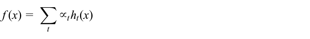
To provide a clearer illustration, consider the example in the Figure 2 below.²⁵ Multiple models are utilized, and their predictions are weighted to form the final ensemble prediction. As the boosting process progresses, well-performing models are emphasized, leading to an ensemble with improved accuracy.

Figure 2.

Boosting architecture.

The function of bagging is shown as follows:

f (x) = \frac{1}{B} \sum_{B = 1}^{B} f_{b (x)}

where $f_{b (x)}$ represent weak learners, $\frac{1}{B}$ generates bootstrapping sets.

Stacking

Smyth and Wolpert introduced stacking, 1997, is an ensemble learning method that combines multiple base models by training a meta-model on their predictions.²⁶ The base models serve as input to the meta-model, which learns to make the final prediction based on their outputs (Figure 3).

Figure 3.

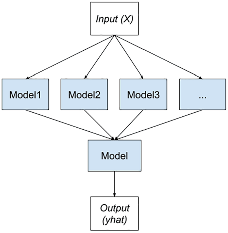
Stacking architecture.

The function of stacking is shown as follows

f_{s} (x) = \sum_{n = 1}^{n} a_{i} f_{i} (x)

In the pseudo code, shown Appendix B section, base classifiers are trained on the training data, and their predictions are used to train the meta-classifier. The meta-classifier then makes the final prediction based on the outputs of the base classifiers. This stacking process enables the ensemble to benefit from the diverse insights of individual models, resulting in enhanced overall predictive accuracy.

Bagging

Bagging was introduced by Breiman, 1996, also known as bootstrap aggregating, is an ensemble learning technique that involves creating multiple datasets by down-sampling the original data with replacement.²⁵ Each dataset is used to train an individual model, typically of the same type, such as decision trees. During the combination stage, the predictions from all individual models are aggregated through a majority vote for classification tasks or averaging for regression tasks. This process aims to reduce variance and improve the overall predictive performance of the ensemble.

For a more intuitive understanding, let’s consider the example in the following Figure 4, where the base model used is a decision tree.

Figure 4.

Bagging architecture.

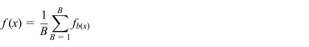
The function of bagging is illustrated as follows:

f (x) = \sum_{t} \propto_{t} h_{t} (x)

Where $f (x)$ represent the strong classifier, $h_{t} (x)$ several weak classifiers. The strong classifier creates a model from the training data, and then creates a second model that first tries to rectify the mistakes of the first model $\propto_{t}$ .

In the pseudo code, as illustrated in the Appendix C section, multiple base classifiers are trained on random bootstrap samples of the training data. The base classifiers’ predictions are then combined using majority voting (for classification tasks) to produce the final ensemble prediction. The Bagging algorithm aims to reduce variance and improve the overall predictive performance of the ensemble.²⁷

Random subspace

Random Subspace, also known as Feature Bagging, is a variation of bagging that introduces diversity among the base models by training each model on a random subset of features (columns) from the training data. It helps prevent overfitting and improves generalization (Figure 5).²⁸

Figure 5.

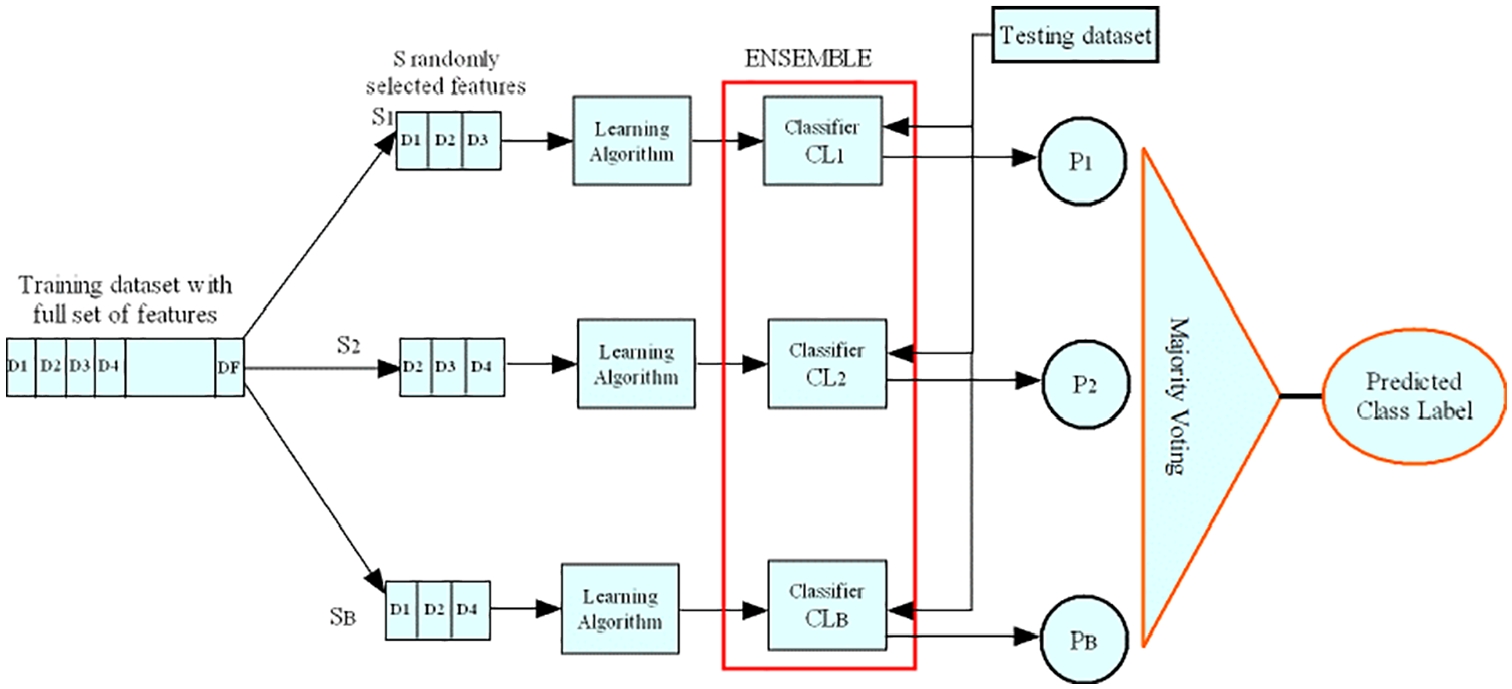
Random subspace architecture.

Suppose you have a dataset represented as a matrix X, where each row corresponds to a data sample, and each column corresponds to a feature:

X = n_samples \times n_features matrix

The Random Subspace method can be mathematically represented as follows:

Define a binary mask matrix M, where each entry $M [i, j]$ is either 0 or 1, indicating whether a feature is selected (1) or not (0):

M = n_features \times n_features matrix

Randomly generate the binary mask matrix M such that exactly n_selected_features columns have the value 1 (indicating feature selection), and the remaining columns have the value 0 (indicating feature exclusion).

Multiply the original dataset X by the binary mask matrix M to obtain the reduced feature subspace X_subspace:

X_subspace = X \times M

Where:

X_subspace is a new dataset containing a subset of features from the original dataset X, with dimensions n_samples × n_selected_features.

The process of randomly generating M ensures that different subsets of features are selected in each iteration, introducing diversity in feature subsets.

The final result, X_subspace, can then be used for model training or other machine learning tasks, focusing only on the selected subset of features

In the pseudo code, as shown in the Appendices section, multiple base classifiers are trained on random subsets of features from the training data. The same feature subset used during training is also applied for generating predictions on the test data. The base classifiers’ predictions are then combined using majority voting (for classification tasks) to produce the final ensemble prediction. The Random Subspace algorithm aims to enhance model diversity and generalization performance.²⁹

Data description

The dataset used in this study was generated from a highly sophisticated simulator of Gas Turbines (GT) mounted on a Frigate, featuring a Combined Diesel electric And Gas (CODLAG) propulsion plant.⁴ The simulator comprises various interconnected blocks, including Propeller, Hull, GT, Gear Box, and Controller, which have been meticulously developed and fine-tuned based on numerous real propulsion plants over time. As a result, the available data closely resemble those of an actual vessel see Figure 6.

Figure 6.

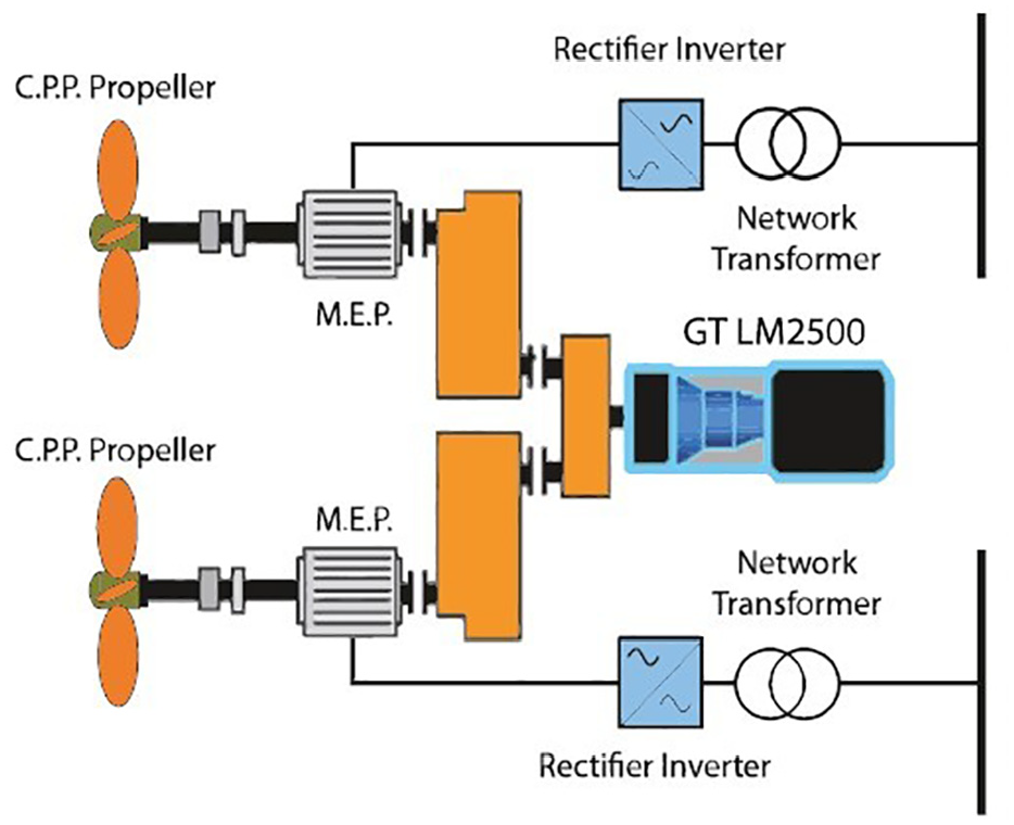
CODLAG propulsion system.

The dataset reflects the behavior of the propulsion system, and it is characterized by two essential parameters: the compression degradation coefficient (kMc) and the turbine degradation coefficient (kMt). Each conceivable degradation state is represented by a combination of these two coefficients (kMc, kMt). To ensure a comprehensive representation, the decay of the compressor and turbine was sampled using a uniform grid with a precision of 0.001, resulting in a finely detailed portrayal.

Specifically, the compressor decay state was discretized in the domain [1, 0.95], while the turbine coefficient was explored in the domain [1, 0.975]. The range of feasible ship speeds was also investigated, spanning from 3 knots to 27 knots, with a granularity of representation set at three knots.

Throughout the experiments, a series of 16 features were measured and recorded, serving as indirect representations of the system’s state subject to performance decay. These measures were collected across the parameter space, contributing to the dataset’s comprehensiveness and significance in analyzing the behavior of the propulsion system.⁴

The dataset comprises a 16-feature vector, representing the Gas Turbine (GT) measures at a steady state of the physical asset. These features are as follows:

Lever position (lp) []

Ship speed (v) [knots]

Gas turbine shaft torque (GTT) [kN m]

Gas turbine rate of revolutions (GTn) [rpm]

Gas Generator rate of revolutions (GGn) [rpm]

Starboard Propeller Torque (Ts) [kN]

HP Turbine exit temperature (T48) [C]

GT Compressor outlet air temperature (T2) [C]

HP Turbine exit pressure (P48) [bar]

GT Compressor outlet air pressure (P2) [bar]

Gas turbine exhaust gas pressure (Pexh) [bar]

Turbine Injection Control (TIC) [%]

Fuel flow (mf) [kg/s]²⁸

Before applying machine-learning algorithms, three features with fixed values were removed from the dataset. These features were:

GT Compressor inlet air pressure (P1) [bar]

GT Compressor inlet air temperature (T1) [C]

Port Propeller Torque (Tp) [kN]

The removal of these features was necessary to avoid redundancy and eliminate any potential influence of fixed-value features on the model’s performance. With the modified dataset, machine learning algorithms were then applied to perform data analysis and prediction tasks (Figure 7).

Figure 7.

Gas turbine scheme.

The design and methodology of the technique used

In our research, we conducted a classification task to categorize the phases of the GT Compressor decay state coefficient and the GT Turbine decay state coefficient. The objective is to analyze and identify the degradation state of the Gas Turbine (GT) components accurately.

To achieve this, we defined four distinct classes for each decay state coefficient, based on specific threshold values. For the GT Compressor decay state coefficient, the classes were defined as follows:

Class 1: When the GT Compressor decay state coefficient equals 1.

Class 2: When the GT Compressor decay state coefficient is 0.99.

Class 3: When the GT Compressor decay state coefficient ranges from 0.97 to 0.98.

Class 4: When the GT Compressor decay state coefficient ranges from 0.95 to 0.96.

Similarly, for the GT Turbine decay state coefficient, the classes were defined as:

Class 1: When the GT Turbine decay state coefficient equals 1.

Class 2: When the GT Turbine decay state coefficient is 0.99.

Class 3: When the GT Turbine decay state coefficient is 0.98.

Class 4: When the GT Turbine decay state coefficient is 0.97.

We utilized this well-defined classification scheme to accurately identify the degradation levels of the GT components and gain insights into the behavior of the Gas Turbine under different decay states. By using appropriate machine learning algorithms, we were able to effectively classify the decay state coefficients and extract valuable information for further analysis and decision-making.

The methodology employed in this classification task, along with the precise definition of classes, enabled us to carry out a comprehensive and detailed investigation into the degradation behavior of the Gas Turbine components.

In our study, we focused on analyzing and addressing two critical failures related to the Gas Turbine (GT) components:

GT Compressor decay state coefficient

The GT Compressor decay state coefficient was of primary interest in our investigation. To effectively assess the degradation level of the GT Compressor, we categorized its decay state coefficient into four distinct levels:

Very Bad State: Represents a severe deterioration in the GT Compressor decay state, characterized by a coefficient ranging from 0.95 to 0.96.

Bad State: Indicates a noticeable degradation in the GT Compressor decay state, with a coefficient ranging from 0.97 to 0.98.

Acceptable State: Signifies a moderate level of decay in the GT Compressor, with a coefficient equal to 0.99.

Normal State: Corresponds to an ideal and fully functional GT Compressor with a decay state coefficient of 1.

GT Turbine decay state coefficient

The GT Turbine decay state coefficient was another critical aspect of our research. To comprehensively evaluate the degradation level of the GT Turbine, we divided its decay state coefficient into four distinct levels:

Very Bad State: Represents a significant deterioration in the GT Turbine decay state, with a coefficient equal to 0.97.

Bad State: Indicates a notable degradation in the GT Turbine decay state, characterized by a coefficient equal to 0.98.

Acceptable State: Signifies a moderate level of decay in the GT Turbine, with a coefficient equal to 0.99.

Normal State: Corresponds to an optimal and fully functional GT Turbine with a decay state coefficient of 1.

By delineating these specific failure levels for both the GT Compressor and GT Turbine decay state coefficients, our research enabled a comprehensive understanding of the degradation patterns, facilitating precise diagnostics and efficient decision-making for maintaining and optimizing the Gas Turbine’s performance.

Results and discussion and comparative studies

To address the issues of overlearning and overfitting caused by varying load/speed condition, various types of rotating machine components and single/multiple faults, small/Big data-set, the framework of proposed approach are presented in Figure 8. This flowchart illustrates the step-by-step process of our ensemble learning approach, which involves utilizing Bagging, Boosting, and Stacking techniques to analyze and classify the degradation state coefficients of the GT Compressor and GT Turbine. Additionally, Random Subspace is employed to enhance model diversity and prevent overfitting during the classification process.

Figure 8.

Proposed multi-fault diagnosis framework.

Simple learning scenario

In the initial phase of our study, we considered using simple learning algorithms, such as Support Vector Machines (SVM) and Naïve Bayes, to test each simple learning machine individually in term of stability and accuracy of the GT Compressor and GT Turbine decay state coefficients. However, we were uncertain about the effectiveness of the results achievable with these standalone classifiers. As anticipated, the accuracy of each classifiers was relatively differentiated, as demonstrated in the below tables.

The obtained results show in the Tables 1 and 2 a considerable variability, with SVM, LS-SVM, and Naïve Bayes yielding weak performance, while Decision Tree and k-Nearest Neighbors (KNN), with varying numbers of neighbors, achieved relatively accepted accuracy, with rating average 90%.

Table 1.

GT turbine prediction results using a simple learning algorithms.

Test	SVM	LS_SVM	KNN	Decision tree	Naïve Bayes	Linear Discernment analyses
1	34.4876	31.0541	85.9816	90.7847	35.9955	82.8540
2	35.7855	33.4728	87.0427	90.7288	38.7601	82.1000
3	34.1801	31.1986	87.1824	90.7568	34.2642	83.2170
4	35.6205	31.5752	86.8193	90.0307	38.6205	83.9710
5	34.0433	32.1404	86.0933	90.5334	37.0288	83.0494
6	34.8857	33.0010	87.5454	90.3937	35.8838	82.9657
7	34.8313	32.8670	86.5959	91.0360	37.4756	82.6585
8	34.4404	32.3604	87.21033	90.4496	37.5593	83.8313
9	34.1971	30.3020	86.8193	90.5054	38.7601	83.4404
10	35.8126	31.0220	86.9310	90.8126	37.1963	82.8819
Min	34.0433	30.3020	85.9816	90.0307	34.2642	82.1000
Mean	34.8284	31.8993	86.8221	90.6032	37.1544	83.0969
Max	35.8126	33.4728	87.5454	91.0360	38.7601	83.9710
STD	0.6845	1.0289	0.4891	0.2815	1.4492	0.5524

The bold values represents the best results obtained with the classifiers.

Table 2.

GT compressor prediction results using a simple learning algorithms.

Test	SVM	LS_SVM	KNN	Decision tree	Naïve Bayes	LDA
1	41.6643	32.0220	91.5108	92.7395	42.6979	78.8327
2	40.6231	34.9110	91.9017	92.1251	44.2893	79.7822
3	41.2101	33.1610	90.7568	92.2368	45.2667	79.0841
4	41.1079	32.4179	90.1703	92.4540	42.5300	79.5588
5	42.0110	31.4210	90.8964	91.8179	41.2455	80.1173
6	40.6132	32.4061	90.5064	92.0972	44.1776	79.0841
7	41.2193	32.0893	92.1810	92.3764	39.2069	79.8660
8	41.0708	31.0178	91.0018	91.8738	39.3466	79.9218
9	41.3300	32.2170	91.7342	92.5998	38.6484	78.6931
10	40.1718	32.7340	91.3991	92.7395	41.1274	80.3686
Min	40.1718	31.0178	90.1703	92.7395	38.6484	78.6931
Mean	41.1022	32.4397	91.2058	92.3060	41.8536	79.5309
Max	42.0110	34.9110	92.1810	92.7395	45.2667	80.3686
STD	0.5328	1.0605	0.6451	0.3325	2.3241	0.5738

The bold values represents the best results obtained with the classifiers.

The assessment of simple classifiers on the turbine dataset as illustrated in Table 1, including a comprehensive analysis of 10 independent tests, reveals compelling information. A clearly shows in the results for each classifier, that the Decision Tree achieves a remarkable average accuracy of 90.6032%, with a particularly low standard deviation of 0.2815.

These results demonstrate that the Decision Tree its robust predictive abilities, making it the optimal choice among the classifiers evaluated for the prediction of turbine-related phenomena.

A thorough examination of the performance of simple classifiers on the compressor dataset, carried out over the 10 entire tests, provides insightful information. The results obtained for each classifier show a clearly distinguishable that the Decision Tree are successfully predicted With accuracy of 92.3060%, and with low stability of 0.3325.

We concluded that, the obtained results from the simple learning especially the DT could be considered satisfactory in some cases. By contrast, considering the sensitivity and real-world application as presented in our study where the safety and productivity are the priority objectives, we recognized the need more robust, stabile and accurate predictions.

Ensemble learning scenario

In this subsection, by applying four different ensemble-learning methods, we focused on the decay state coefficients of the GT compressor and the GT turbine. Among these methods, boosting proved the most effective for the GT turbine’s decay state coefficient, while stacking demonstrated superior performance for the GT compressor’s decay state coefficient. In our quest for the best possible results, we conducted extensive experiments with different learners until we arrived at the optimal combination of classifiers. Specifically, for the GT turbine decay state coefficient, the Boosting method proved to be the most efficient selection, using a set of 200 decision trees. On the other hand, for the GT compressor decay state coefficient, the Stacking approach proved highly effective, involving a diverse set of learners.

In the Stacking ensemble for GT Compressor, we carefully selected a range of learners, including k-Nearest Neighbors (kNN) with different values of K-nearest neighbors (3, 7, and 9), Random Forest with 200 decision trees, Linear Discernment Analysis, and Decision Tree as weak learners, in conjunction with Random Forest (200 trees) as the meta learner. The inclusion of these specific learners in the Stacking ensemble was based on their individual strong performances as standalone classifiers during the preliminary single-learning phase.

By combining the power of Boosting and Stacking, we successfully addressed the GT Turbine and GT Compressor decay state coefficients, enabling accurate and robust predictions of the Gas Turbine’s degradation levels. The strategic integration of Ensemble Learning approaches enabled us to achieve exceptional predictive accuracy and enhanced insights into the degradation behavior of the Gas Turbine components.

As mentioned previously, our study including a comprehensive analysis of 10 independent tests reveals compelling information. Firstly, in GT Turbine as illustrated in the Table 3, start with Bagging, which averaged 94.0022% accuracy. These results show that, the standard deviation (STD) a relatively higher, Bagging demonstrated steadily of 10 tests improved accuracy compared to the simple learning. Notably, Stacking and Random Subspace further improved predictive performance 95.4303% and 95.1249%, with low and high stability STD, respectively.

Table 3.

GT turbine prediction results using Ensemble learning algorithms.

Test	Bagging	Stacking	Randomsubspace	Boosting
1	95.2248	95.3021	94.9735	96.3139
2	94.0519	95.9176	95.7833	96.2863
3	94.3033	95.9509	95.4203	96.3071
4	93.7448	95.0572	95.6716	96.3037
5	93.5214	95.3086	93.6942	96.2940
6	94.2753	95.4203	95.1969	96.2832
7	94.6104	95.1689	95.2527	96.2991
8	94.1916	95.7554	94.7501	96.3021
9	94.3033	95.1969	94.8365	96.3100
10	92.7957	95.2248	95.6700	96.2801
Min	95.2248	95.0572	93.6942	96.2801
Mean	94.0022	95.4303	95.1249	96.2979
Max	92.7957	95.9509	95.7833	96.3139
STD	0.6921	0.3249	0.6175	0.0117

The bold values represents the best results obtained with the classifiers.

On the other hand, ensemble boosting technique achieved an average of MAX accuracy of 96.3139%, indicating a substantial improvement over ten tests of previous methods, and also the Boosting classifier enhance the stability value, which is clearly the best prediction with low value 0.0117%.

In order to demonstrate the effectiveness of the proposed approach, an analysis of the four ensemble learning models presented in a confusion matrix of each class (4 classes of GT turbine) are illustrated in Figure 9. This demonstrates that the fault prediction accuracy of the proposed algorithms leads to the accurate identification observations with minor misclassification errors. The suggested algorithm has an impressive classification performance and can considerably improve the GT turbine fault diagnosis capabilities.

Figure 9.

Confusion matrix of ensemble learning models of GT turbine.

As shown in the Table 4, the bagging, random subspace, boosting, and stacking each of those techniques achieve highly creditable average accuracy rates of 94.0834%, 94.5657%, 94.5624%, and 95.1843%, respectively. That these methods have a relatively narrow range of standard deviations (STDs) between 0.090 and 0.400 is impressive, confirming their consistent and reliable performance characteristics.

Table 4.

GT compressor prediction results using Ensemble learning algorithms.

Test	Bagging	Stacking	Random subspace	Boosting
1	94.2753	95.1200	94.4708	95.5040
2	94.2195	95.1689	94.5546	94.4150
3	94.0799	95.4203	94.6663	94.6663
4	94.1636	95.1812	94.4429	94.5825
5	94.0240	95.1103	94.6384	94.3591
6	94.5267	95.1902	94.7221	94.2474
7	94.1357	95.1922	93.9402	94.8006
8	93.8844	95.1520	94.7221	94.5267
9	93.6610	95.1401	94.6942	94.2472
10	94.0559	95.1680	94.8059	94.2753
Min	93.6610	95.1103	93.9402	94.2472
Mean	94.0834	95.1843	94.5657	94.5624
Max	94.5267	95.4203	94.8059	95.5040
STD	0.2863	0.0875	0.2481	0.3800

The best results obtained in bold.

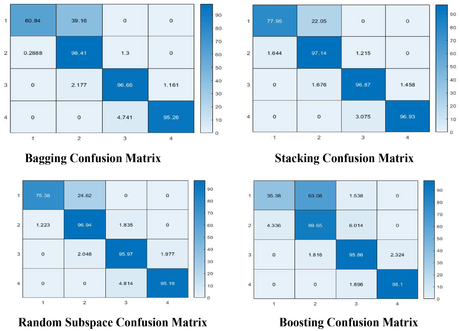
In addition, a same analysis has been made of four ensemble learning models presented in a confusion matrix of each class (4 classes of GT compressor) are illustrated in Figure 10. This study demonstrates that the fault prediction accuracy of the proposed algorithms successfully identifies with minor classification errors. The proposed approach has an incredible classification impact and can enhance the GT compressor fault diagnosis abilities.

Figure 10.

Confusion matrix of ensemble learning models of GT Compressor.

Evaluating ensembles learning models

Predictive performance metrics have been the most important criterion for choosing classifier performance. In addition, predictive performance metrics are generally recognized as a practical way of comparing machine-learning algorithms. To evaluate an ensemble model, there are a number of common measures, such as Precision, Specificity, and sensitivity as shows below:

(a) Boosting method

Class 1: precision = 81.14, sensitivity = 77.97, specificity = 99.32.

Class 2: precision = 96.38, sensitivity = 97.14, specificity = 97.66.

Class 3: precision = 97.22, sensitivity = 96.86, specificity = 98.27.

Class 4: precision = 97.06, sensitivity = 96.92, specificity = 98.82.

(b) Stacking matrix

Class 1: precision = 85.96, sensitivity = 75.38, specificity = 95.53.

Class 2: precision = 95.41, sensitivity = 96.94, specificity = 97.31.

Class 3: precision = 95.83, sensitivity = 95.97, specificity = 97.27.

Class 4: precision = 96.1, sensitivity = 95.18, specificity = 99.01.

We observed from Figures 11 and 12 represented the results of evaluation metrics of four classes of the boosting method and stacking matrix, proving that this classifier gives the best classification model in terms of performance and stability.

Figure 11.

Evaluation matrix of boosting method.

Figure 12.

Evaluation matrix of stacking method.

Concluded that, the proposed criteria based on ensemble learnings does not only improve the overall accuracy but also enhance the classification of each class of faults, making it a more effective method for fault diagnosis in Naval Propulsion Systems.

Conclusion

In this study, we embarked on a rigorous exploration aimed at enhancing the accuracy and predictive prowess of fault diagnosis in Gas Turbines (GT) through the utilization of Ensemble Learning techniques. Acknowledging the limitations of traditional, standalone classifiers, we set out to unravel the untapped potential of combining multiple learners to create a cohesive and robust predictive framework. Our investigation commenced with a meticulous analysis of simple learning algorithms, where classifiers like Support Vector Machines (SVM), Naïve Bayes, and Decision Tree were scrutinized in isolation. While these methods provided valuable insights, their individual performance often fell short of our expectations, particularly when addressing the intricate nuances of the GT compressor and GT turbine decay state coefficients.

Recognizing the need for an elevated predictive accuracy, we delved into the realm of Ensemble Learning, an approach characterized by the symbiotic collaboration of diverse learners. Bagging, Boosting, Stacking, and Random Subspace emerged as our chosen ensemble methods, each contributing its unique strengths to the predictive landscape. Through a series of intensive experiments and 10 comprehensive trials, the Ensemble Learning methods demonstrated remarkable efficacy in forecasting the degradation levels of both GT compressor and GT turbine. Notably, stacking emerged as a standout performer, showcasing exceptional predictive accuracy and a remarkably low standard deviation.

The pinnacle of predictive excellence was unequivocally attained through the Boosting method, which not only achieved an impressive mean accuracy of 96.2979% but also exhibited unprecedented stability with a negligible standard deviation of 0.0117. These results illuminate the extraordinary potential of Ensemble Learning in addressing the inherent challenges of fault diagnosis in Gas Turbines.

In conclusion, our research underscores the transformative power of Ensemble Learning in fault diagnosis, particularly in the context of complex and critical systems like Gas Turbines. By harnessing the collective intelligence of multiple classifiers, we have unlocked a new realm of accuracy and precision, empowering us to better understand, predict, and optimize the performance of these vital assets. As we advance into an era of ever-evolving technologies, Ensemble Learning stands as a beacon of innovation and insight, poised to revolutionize the field of fault diagnosis and beyond.

Footnotes

Appendices

Handling Editor: Aarthy Esakkiappan

Declaration of conflicting interests

The author(s) declared no potential conflicts of interest with respect to the research, authorship, and/or publication of this article.

Funding

The author(s) received no financial support for the research, authorship, and/or publication of this article.

ORCID iDs

Mohammed Amine Sahraoui

Chemseddine Rahmoune

Ali Damou

Fawzi Gougam

References

Lambert

The challenge: Britain against America in the naval War of 1812. London: Faber & Faber, 2012.

Pal

Datta

Segev

, et al. Condition based maintenance of turbine and compressor of a codlag naval propulsion system using deep neural network. In: 6th international conference on artificial intelligence and applications (AIAP-2019), Vienna, Austria, 27–28 April 2019.

Ibrahim

Mohammed

Al Door

WHA

, et al. Study of the performance of the gas turbine power plants from the simple to complex cycle: a technical review. J Adv Res Fluid Mech Therm Sci 2019; 57: 228–250.

Coraddu

Oneto

Ghio

, et al. Machine learning approaches for improving condition-based maintenance of naval propulsion plants. Proc IMechE, Part M: J Engineering for the Maritime Environment 2016; 230: 136–153.

Sahraoui

Rahmoune

Zair

, et al. Enhancing fault diagnosis of undesirable events in oil & gas systems: a machine learning approach with new criteria for stability analysis and classification accuracy. Proc IMechE, Part E: J Process Mechanical Engineering. Epub ahead of print 15 November 2023. DOI: 10.1177/09544089231213778.

Campora

Cravero

Zaccone

Marine gas turbine monitoring and diagnostics by simulation and pattern recognition. Int J Nav Arch Ocean Eng 2018; 10: 617–628.

Hoang

D-T

Kang

H-J.

A survey on deep learning based bearing fault diagnosis. Neurocomputing 2019; 335: 327–335.

Mellit

Kalogirou

Assessment of machine learning and ensemble methods for fault diagnosis of photovoltaic systems. Renew Energy 2022; 184: 1074–1090.

Wen

Bao

, et al. Fault diagnosis based on deep learning. In: 2016 American control conference (ACC), Boston, MA, USA, 6–8 July 2016, pp.6851–6856. New York: IEEE.

10.

Sazli

MH.

A brief review of feed-forward neural networks. Commun Fac Sci Univ Ankara Ser A2-A3 Phys Sci Eng 2006; 50: 11–17.

11.

Liu

Yang

, et al. A survey of convolutional neural networks: analysis, applications, and prospects. IEEE Trans Neural Netw Learn Syst 2021; 33: 6999–7019.

12.

Alam

Mohamed

Selamat

, et al. A review of recurrent neural network based camera localization for indoor environments. IEEE Access 2023; 11: 43985–44009.

13.

Sagi

Rokach

Ensemble learning: a survey. Wiley Interdiscip Rev Data Min Knowl Discov 2018; 8: e1249.

14.

Damou

Ratni

Benazzouz

DJ.

Intelligent multi-fault identification and classification of defective bearings in gearbox. Adv Mech Eng 2024; 16: 16878132241246673.

15.

Ganaie

Malik

, et al. Ensemble deep learning: a review. Eng Appl Artif Intell 2022; 115: 105151.

16.

Peng

A novel ensemble machine learning for robust microarray data classification. Comput Biol Med 2006; 36: 553–573.

17.

Ahmad

Reynolds

Rezgui

Predictive modelling for solar thermal energy systems: a comparison of support vector regression, random forest, extra trees and regression trees. J Clean Prod 2018; 203: 810–821.

18.

Song

L-K

X-Q

Zhu

S-P

, et al. Cascade ensemble learning for multi-level reliability evaluation. Aerosp Sci Technol 2024; 148: 109101.

19.

Gougam

Afia

Soualhi

, et al. Bearing faults classification using a new approach of signal processing combined with machine learning algorithms. J Braz Soc Mech Sci Eng 2024; 46: 65.

20.

Sahraoui

Rahmoune

Meddour

, et al. New criteria for wrapper feature selection to enhance bearing fault classification. Adv Mech Eng 2023; 15: 16878132231183862.

21.

Rahmoune

Amine Sahraoui

Gougam

, et al. Enhancing air compressors multi fault classification using new criteria for Harris Hawks optimization algorithm in tandem with MODWPT and LSSVM classifier. Adv Mech Eng 2023; 15: 16878132231216208.

22.

Wazid

Das

Chamola

, et al. Uniting cyber security and machine learning: advantages, challenges and future research. ICT Express 2022; 8: 313–321.

23.

Farooq

Ahmed

Akbar

, et al. Predictive modeling for sustainable high-performance concrete from industrial wastes: a comparison and optimization of models using ensemble learners. J Clean Prod 2021; 292: 126032.

24.

Opitz

Maclin

Popular ensemble methods: an empirical study. J Artif Intell Res 1999; 11: 169–198.

25.

Maclin

Opitz

. An empirical evaluation of bagging and boosting. In: Proceedings of the fourteenth national conference on artificial intelligence, AAAI 97, Providence, RI, USA, 27–31 July 1997, pp.546–551. Cambridge, MA: AAAI Press/MIT Press.

26.

Smyth

Wolpert

Linearly combining density estimators via stacking. Mach Learn 1999; 36: 59–83.

27.

Bühlmann

Bagging, boosting and ensemble methods. In: Gentle

Härdle

Mori

(eds) Handbook of computational statistics. Berlin, Heidelberg: Springer, 2012, pp.985–1022.

28.

Tian

Feng

RaSE: random subspace ensemble classification. J Mach Learn Res 2021; 22: 2019–2111.

29.

Kuncheva

Rodríguez

Plumpton

, et al. Random subspace ensembles for fMRI classification. IEEE Trans Med Imaging 2010; 29: 531–542.

Advancing condition-based maintenance of naval propulsion systems with ensemble learning techniques

Abstract

Keywords

Introduction

Ensemble learning

Common ensemble methods

Boosting

Stacking

Bagging

Random subspace

Data description

The design and methodology of the technique used

GT Compressor decay state coefficient

GT Turbine decay state coefficient

Results and discussion and comparative studies

Simple learning scenario

Ensemble learning scenario

Evaluating ensembles learning models

Conclusion

Footnotes

Appendices

Declaration of conflicting interests

Funding

ORCID iDs

References