Sage Journals: Discover world-class research

Abstract

This work presents an advanced structural reliability analysis of circular concrete-filled steel tubular (CFST) members through machine learning and global optimization, together with numerical Monte Carlo simulations (MCS). The artificial neural network (ANN) model is developed and validated against available experimental data. On the basis of monetary cost of materials, the optimal design of CFST members with reliability constraint is formulated and solved by balancing composite motion optimization (BCMO) algorithm. Based on the MCS, reliability analysis is then carried out to calculate the coefficient of variation of optimal design under different loads. Subsequently, a comprehensive prediction simulation, taking account of the uncertainty of experimental data and potential errors from models (ANN, MCS, and BCMO), is performed to generate the statistics on the axial capacity of CFST members. The critical value for the optimal solution is also investigated as a function of the input variables. The results of this study can be applied to achieve a better reliability-based design optimization with minimum cost for the circular CFST columns.

Keywords

Concrete-filled steel tubular members reliability analysis design optimization machine learning out-of-boundary prediction

Introduction

Concrete-filled steel tubular (CFST) members present remarkable characteristics due to combination the advantages of the two constituent phases: the tensile strength of the steel tube and compressive strength of the concrete cylinder. This combination enhances significant members’ structural responses including ductility,^1,2 strength,^3,4 fire resistance,^5,6 load-bearing capacity,^7–9 earthquake resistance,^10,11 energy-absorption capacity,^12,13 etc. Thus, many researchers and engineers have dedicated a great deal of attention to the axial strength of CFST columns.¹⁴ have performed compression tests on both hollow steel and composite members. For hollow steel members, they observed both inward and outward local instabilities. On the other hand, for composite members, only outward local buckling was seen, proving that the concrete cylinder prevents inward deformation of the steel. As a result, the composite columns were stronger than steel alone, because the wall tended only to buckle toward the outside. The same conclusion has been reached by other researchers – for instance,^15–17 etc. CFST columns have been employed in many types of infrastructure, such as bridges, buildings and underground facilities.^11,18

It should be noted that although the design for CFST columns is available in existing standards including American,¹⁹ British,²⁰ European,²¹ and Australian/New Zealand,²² however, these standards do not consider various ranges of material strengths and/or geometrical parameters.^23–26 For example, the yield stress of steel and compressive strength of concrete limit to 460 MPa and 50 MPa for Eurocode 4 and those of AISC 360-16 are 525 MPa and 69 MPa, respectively. Among them, AS/NZS 2327 allows the use of high strength steel and concrete up to 690 MPa and 100 MPa. Moreover, CFST structures are part of a field of research that has attracted a great deal of attention over recent decades, with researchers/engineers seeking economical and optimized constructions. Many optimization studies have proposed optimal designs for structural members at minimal cost.²⁷ optimized fiber-reinforced CFST members based on dimensions of columns and percentage of reinforcements.²⁸ designed a cantilever retaining wall with minimal cost based on the gray wolf optimization technique. Other optimization techniques have been successfully employed for optimal design of structural members with minimal cost: particle swarm optimization,²⁹ biogeography-based optimization,³⁰ etc. However, to the best of the authors’ knowledge, optimal design of circular CFST columns at minimal cost has rarely been investigated.²⁷

One crucial aspect is the reliability to predict the column’s capacity within a certain specified confidence interval.^31–37 Even with modern, advanced analysis tools which are capable of efficiently estimating the capacity of complex structures under given conditions, the ultimate loads, geometric, and material nonlinearities are still not easily predictable.³⁸ It is worth noticing that in practice, structural elements may have imperfections in different forms and at different levels due to manufacturing, transportation, and other constructional processes.^33,39,40 Indeed, structural element capacity is remarkably difficult to predict and assess. First, geometrical imperfections could occur during the manufacturing processes, mostly in the cross-section or along the length of structural members; or there may be fluctuations of the mechanical properties of the constituent materials. Second, during assembly and/or construction, residual stresses could appear within the structural elements. Finally, eccentricity of the compressive loads could also reduce the member’s capacity. Each of the above is a factor that significantly affects the compressive resistance of members, which must be taken into account in the initial design.⁴¹ Moreover, previous works^40,42,43 have shown that failing to consider the effect of imperfections may affect the prediction of CFST members’ capacity, leading to potential risks in practice at both the micro- and macroscopic scales. Consequently, statistical analysis and uncertainty quantification should be conducted to answer the question: how accurate are the predicted capacity values when applying given material properties, geometrical data, and boundary conditions?^44–46

Many studies have been focused on this problem for CFST column revealing the natural complex of the problem and weakness of some codes. Kang et al.⁴⁷ found that the complication of predicting load capacity of a composite member and more test samples were required for such member compared to a non-composite one. Thai et al.⁴⁸ provided a thorough study of reliability assessment of current codes for CFST columns with a globally collected database. This study also figured out that the current EC4 code should be extended to be up-to-date.

Besides, there are several methods to estimate the ultimate load of structural CFST members under different types of loads (see Kang et al.,⁴⁷ Moon et al.,⁴⁹ Güneyisi et al.,⁵⁰ and Ahmadi et al.⁵¹). Regression machine-learning techniques have been widely used recently to solve this complicated problem. Thanh Duong et al.⁵² developed high-quality ANN model to predict the load capacity of CFST column with R² is up to 0.9899. Naser et al.⁵³ used genetic algorithms and gene expression programing for improving the accuracy of prediction. Lee et al.⁵⁴ used Categorical Gradient Boosting algorithm and compared the results with those from AISC 360-16, Eurocode 4, and AS/NZS 2327. Zarringol and Thai⁵⁵ predicted of the load-shortening curve of CFST columns using ANN-based models. Coupling with the use of machine learning models, reliability assessment for the CFST columns is much more challenging with the unavoidable model uncertainty.^56,57 Besides, there is an evidence of the weakness of these machine learning models such as the quality degradation for the out-of-boundaries prediction.⁵⁸ Unfortunately, the uncertainty of machine-learning model is commonly neglected in many cases.

Generally, this paper fills the gap by proposing, a novel comprehensive investigation study for optimizing the design of circular CFST columns, incorporating a data-driven model and reliability constraints. Section “Experimental database and research methodology” introduces the experimental database and research methodology, including ANN, Monte Carlo Simulation (MCS), and Balancing Composite Motion Optimization (BCMO) as well as optimization with reliability constraint. Finally, Section “Results and discussions” presents the results and discussion, including prediction, design optimization, and uncertainty quantification for CFST members. The proposed method allows us to obtain a comprehensive picture of the reliability of CFST members, where structural uncertainties are considered.

Experimental database and research methodology

Experimental database

In this work, 1245 axially loaded circular CFST column tests were gathered from Thai et al.,⁵⁹ which was mostly from two well-recognized sources Goode and Lam⁶⁰ and Denavit Mark et al.⁶¹ The selection of tests was based on the following criteria: (i) only monotonic uniaxial compression was considered; (ii) the specimens were fully loaded; and (iii) the specimens did not include internal steel reinforcement, shear stub, and tab stiffeners. Table 1 gives a summary of statistical input variables of the dataset. Histograms of variables are given in Appendix A. In addition, correlation coefficients between measured axial capacity and input variables are also given in Table 2. More details of the database can be found in Thai et al.⁵⁹

Table 1.

Descriptive statistics of collected database.

Parameter	Cross-section outside diameter	Wall thickness	Ratio of wall thickness and outside dimension	Length of column	Steel yield stress	Concrete cylindrical compression strength	Measured axial capacity
Notation	D	t	t/D	L	f_y	f’_c	p
Unit	mm	mm	–	mm	MPa	MPa	kN
Count	1245	1245	1245	1245	1245	1245	1245
Mean	158.5169	4.3062	0.0306	1060.0743	336.5337	47.9701	2349.5794
Std*	105.4211	2.4519	0.0166	1005.2827	90.8906	29.7992	4042.2907
Min	44.4500	0.5200	0.0045	152.3492	178.2800	7.7938	45.2000
25%	108.0000	2.7400	0.0200	397.0000	276.0000	28.9247	703.3000
50%	127.3000	4.0000	0.0300	662.0000	325.0000	39.2000	1244.6000
75%	178.0000	5.0000	0.0370	1250.0000	365.0000	55.8979	2253.0000
Max	1020.0000	16.5400	0.1347	5560.0000	853.0000	177.8360	46,000.0000

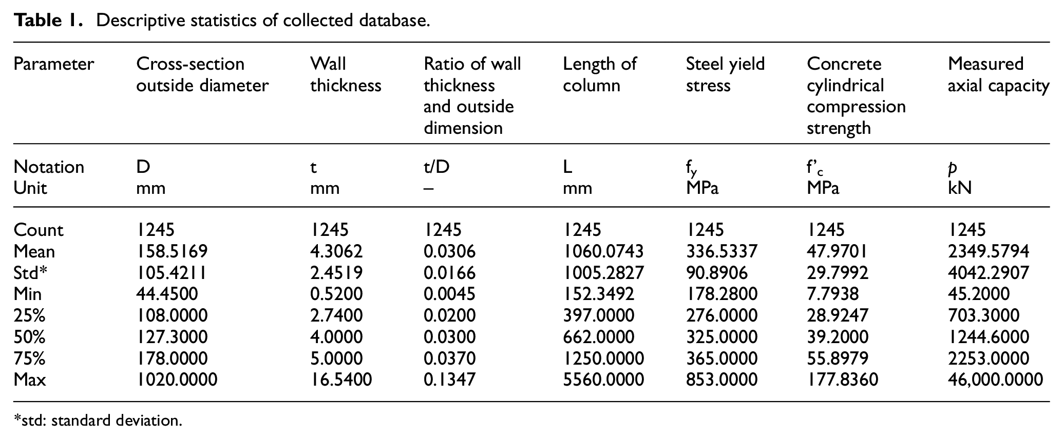
std: standard deviation.

Table 2.

Linear statistical correlation coefficient r of the database (including a value-color scale) (see Appendix B for details).

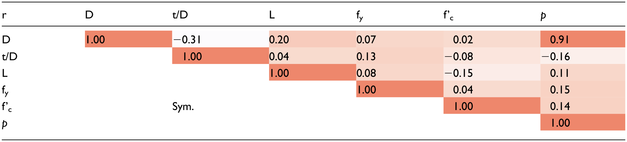
Note. In a correlation matrix, shaded cells typically highlight specific correlations based on their values or significance levels. These shadings often serve to help users quickly identify patterns and relationships between variables.

Artificial neural network (ANN)

The data-driven model relies on labeled database to predict the variables of interest. Conventionally, the database is first split into training and testing datasets. The aim of the training process is to minimize the error between predicted values and the labels in the training set. In the case of ANNs, each of them is a system containing nodes, with weighted links between such nodes. ANNs are divided into layers including input layer, hidden layer(s), and output layer, with nodes in one layer connected to nodes in the previous layer. The training process is triggered at the input layer, with parts of the training dataset or so-called batch. These signals are propagated through the network by a mathematical combination of input signals and activation function. The training dataset is “fed” through the network repeatedly. The weights in an ANN are adjusted during the training process by backpropagation, so the error is minimized after a given number of iterations. Once the ANN is developed, the system is tested and validated by predicting the variable of interest in the test dataset and comparing the results with the corresponding labels on the test dataset.

Monte Carlo simulation (MCS)

For the MCS, once the distributions of the inputs are found or assumed by the law of large numbers, an unlabeled database is established with n samples, each of them is randomly generated corresponding to their distribution.^62,63 Thus, the MCS requires a substantial number of runs to obtain a meaningful result. Unfortunately, increasing the number of trials in the MCS is computationally expensive, especially in the case of optimization. In this paper, it is assumed that input variables including D, t/D, f_y, and f_c, are random variables following normal distributions. The length of column, L, is practically considered as a known and deterministic variable due to the design task. A database of input variables, which is used to predict column strength P by ANN, is randomly generated with the assumed means and standard deviations, std. The stochastic characteristics of n samples of P are observed and the function f = P-N is calculated to determine the number of negative values, n_f, which have an applied load greater than the capacity of the column. The failure probability of the CFST column is then found by equation (1):

P_{f} = \frac{count [(P - N) \leq 0]}{n} = \frac{n_{f}}{n}

(1)

Optimization with reliability constraint and data-driven model

This paper uses an objective function, OF, representing the monetary cost of the column per unit strength, which can be expressed as:

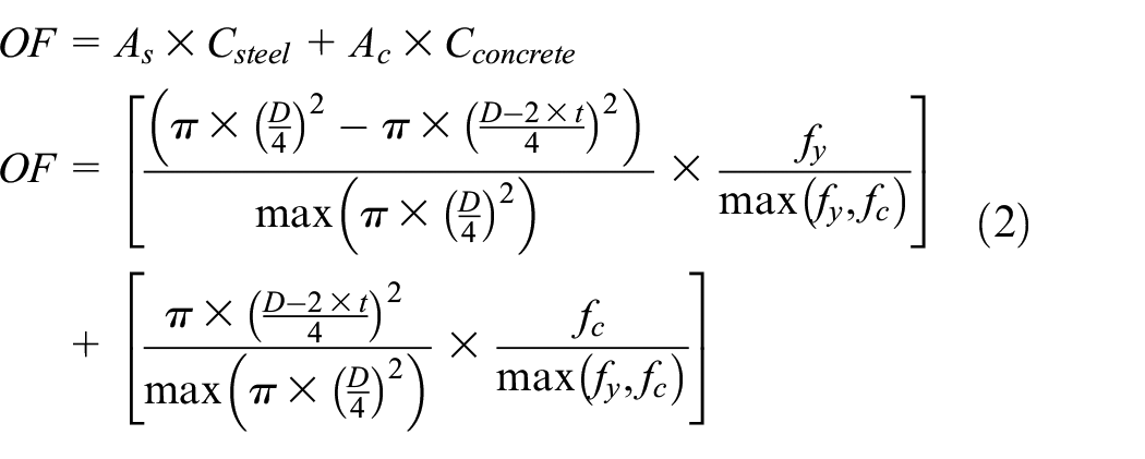
\begin{matrix} OF = A_{s} \times C_{steel} + A_{c} \times C_{concrete} \\ OF = [\frac{(π \times {(\frac{D}{4})}^{2} - π \times {(\frac{D - 2 \times t}{4})}^{2})}{max (π \times {(\frac{D}{4})}^{2})} \times \frac{f_{y}}{max (f_{y}, f_{c})}] \\ + [\frac{π \times {(\frac{D - 2 \times t}{4})}^{2}}{max (π \times {(\frac{D}{4})}^{2})} \times \frac{f_{c}}{max (f_{y}, f_{c})}] \end{matrix}

(2)

where A_s and A_c are the areas of steel and concrete normalized by the maximum area of the cross-section in the database; C_steel and C_concrete are the costs of steel and concrete with the monetary values represented by the strength of materials; $max (f_{y}, f_{c})$ is the maximum strength of steel and concrete in the database, which is equal to 853 MPa in this paper.

The reliability constraints are established from the column failure probability (P_f) which is determined by conventional Monte Carlo simulation (MCS) and does not exceed a given threshold P_fmax (e.g., 0.01 or 0.05). For each trial in the simulation, the axial load capacity of the column is calculated from a database driven model, trained on an experimental database.

The optimization problem in this paper can be stated as below. The notations µ, std and CoV represent mean, standard deviation and coefficient of variation.

- Given an applied axial load N, column length L, and coefficients of variation CoV of the design parameters (std_D, std_t/D, std_fy, and std_f’c);

- Find µ_D, µ_t/D, µ_fy, µ_{f’_c} which minimize OF in equation (1)

- Subjected to: P_f≤Pr_max;

- where: P_f is obtained by Monte Carlo simulation with the load-bearing capacity of the column obtained by a data-driven model.

Balancing composite motion optimization (BCMO)

Proposed by Le-Duc et al.,⁶⁴ the first step of the BCMO algorithm is similar to other metaheuristics, with the creation of the initial population. In this paper, individuals in the population are ranked based on objective function (OF). The composite motion of the i^th individual in the population will depend on two critical points. The first one is the minimum point of the OF, which is represented by the instant global optimization point, X_oin. To avoid early termination of the algorithm due to premature convergence, X_oin is chosen between the performance of the best individual in the previous generation and an individual which extracts information from the current generation. The second one is a randomly chosen individual point which has better performance than the i^th individual. The process of extracting information and searching for motion is repeated until the pre-set maximum number of generations is reached.

The advantage of the BCMO is that the number of parameters is limited by the number of individuals, and maximum number of generations is used as the stop criterion. This algorithm is also tested in this study, revealing its computational efficiency. This reduction in the computational cost is particularly useful in a combination of optimization and reliability assessment with MCS, and thus has been chosen from among various other metaheuristic algorithms.

Uncertainties

The incorporation of ANN and MCS together in the optimization algorithm leads to the accumulation of errors from each individual model. The errors from the MCS and BCMO can be mitigated with improved computational power while that from the ANN model is taken into account by adding a margin of error in each run of the simulations or prediction of column capacity in equation (3). By using approximation, the unknown error of the ANN model is replaced by the mean and standard deviation of error on the test dataset. As expected, the appearance of the error from ANN models increases the value of the objective function, OF.

\begin{matrix} P = P_{ANN} + norm [μ_{error, ANN}, st d_{error, ANN}] \\ \approx P_{ANN} + norm [μ_{error, test}, st d_{error, test}] \end{matrix}

(3)

where P is the predicted load capacity of the column, P_ANN is the load capacity of the column predicted directly by the ANN model; µ_error,ANN and std_error,ANN are the mean and standard deviation of error of the prediction, assumed to be equal to the mean and standard deviation on the test dataset, µ_error,test, std_error,test.

Boundaries for design optimization variables

It should be noted that developed ANN model in this paper is only valid if the inputs are between the minimum and maximum values in the database. An out-of-boundary input may lead to the explosion of unpredictable errors, similar to an extrapolation prediction. Thus, the input boundary of an ANN model is defined based on the upper bound (UB) and lower bound (LB) of those inputs (i.e., D, t/D, f_y and f_c′) in the database. The j^th input must be within the range [LB_j, UB_j] to guarantee the accuracy of the prediction.

The situation is more complicated because of the incorporation of MCS and ANN to obtain the failure probability. The inputs of the MCS are the mean and standard deviation of diameter: µ_D, std_D; of ratio of wall thickness to diameter: µ_t/D, std_t/D; of yield strength of steel: µ_fy, std_fy and of cylindrical strength of concrete: µ_f’c, std_f’c. Obviously, all predictions by ANN in the MCS should have the inputs within their corresponding bounds.

To preserve this, the minimum bound of the mean input for MCS must be higher than the LB in the data-driven model, and vice versa. The distance between these bounds can be set from the mean, std of the inputs and the probability of out-of-boundary prediction is acceptable. In this study, it is assumed that for the j^th input:

+ The LB of the optimization is m × std_j larger than that of the ANN model;

+ The UB of the optimization is m × std_j smaller than that of the ANN model

where m is a control number relating to the probability of out-of-boundary prediction.

There is a trade-off in the width of the range of input and the probability of out-of-boundary prediction, P_obp, occurred. If a large value of m is chosen, the higher probability of within-boundary prediction is obtained. For example, if m = 3 is chosen then the probability of out-of-boundary prediction is 0.00135, when the diameter is a normally distributed variable. If m = 2 then this value is 0.02275. However, this leads to the narrowing down of input boundaries for design variables of the optimization. The boundary of the mean of the j^th input is reduced from [LB_j, UB_j] to [LB_j + m × std_j, UB_j − m × std_j], where m is the critical values deciding the width of such range. The UB and LB of mean of the j^th input, LB_mean,j, UB_mean,j, are mathematically expressed in equation (4) below:

\begin{matrix} L B_{mean, j} = L B_{j} + m \times st d_{j} = L B_{j} + m \times Co V_{j} \times μ_{j} \\ \approx L B_{j} + m \times Co V_{j} \times L B_{j} = L B_{j} (1 + m \times Co V_{j}) \end{matrix}

(4a)

\begin{matrix} U B_{mean, j} = U B_{j} + m \times st d_{j} = U B_{j} + m \times Co V_{j} \times μ_{j} \\ \approx U B_{j} + m \times Co V_{j} \times U B_{j} = U B_{j} (1 + m \times Co V_{j}) \end{matrix}

(4b)

where j represents: D or t/D or L or f_y or f’_c.

Figure 1 illustrates the boundaries of diameter in the database: [44.450; 1020] mm. This range is used as the boundary of the ANN model. Because the standard deviation of diameter is unknown, it is assumed here that LB of D in the database (LB_D) is equal to the µ_D. For instance, the range of µ_D for optimization with CoV_D = 0.1, m = 2 is [53.340, 816.0] mm and with CoV_D = 0.1, m = 3 is [57.785, 714.0] mm. Table 3 compares design variable inputs with different values of m. The corresponding value of p is also included with the standard deviation in the database at 4042 kN, as shown in the Supplementary material. In this study, m = 2 is chosen.

Figure 1.

Relationship between the boundaries of the ANN_P model and optimization problem for the diameter.

Table 3.

Boundaries for optimization design variables with CoV = 0.1.

Input	Unit	m = 1 (P_obp = 0.1585)	m = 2* (P_obp = 0.0228)	m = 3 (P_obp = 0.0014)
µ_D	(mm)	[48.895, 918.00]	[53.340, 816.00]	[57.785, 714.00]
µ_t/D	–	[0.0050, 0.1213]	[0.0054, 0.1078]	[0.0059, 0.0943]
µ_L	(mm)	[167.58, 5004.0]	[182.81, 4448.0]	[198.05, 3892.0]
µ_fy	(MPa)	[196.11, 767.70]	[213.94, 682.40]	[231.76, 597.10]
µ_f’c	(MPa)	[8.573, 160.052]	[9.353, 142.269]	[10.13, 124.485]
µ_P**	(MN)	[4087, 41858]	[8129, 37915]	[12172, 33873]

Chosen in this study.

Used with std_P from database (4042 kN in Table 1) for reference of prediction after optimization design.

Variables found.

The proposed framework

Figure 2 illustrates the proposed framework of this study and the interaction of ANN model, MCS, and BCMO. The ANN model is nested in the MCS. To its turn, the MCS is a subroutine of the BCMO. Initially, for developing the ANN model, the database is divided into train set and test set for training and validating process. Using distribution of residual on the test set as the model uncertainty and natural boundaries from minimum and maximum of samples in the database, the lower and upper bounds of the optimization can be set up.

Figure 2.

The proposed framework of reliability-constrained optimization with ANN model.

Once the spaces of design variables are obtained, random mean of the inputs can be generated within the BCMO. With means and known corresponding CoVs, n samples (i.e., n set of inputs for ANN) are generated. Consequently, n values of P are calculated. These values will be compared with applied load, N, to obtain the failure probability (P_f in equation (1)) of each individual in the BCMO. Maintaining this probability to be less than a desired threshold failure probability, Pr_max, is the process of satisfying the constrain for the BCMO. The objective function is calculated from equation (2) with the corresponding µ_D, µ_t/D, µ_fy, and µ_f’c. The BCMO is continuously checked for all individuals in the next generation are between LB_j and UB_j. To the end, means of D, t/D, L, f_y, f’_c, and P corresponding to the minimum of OF are obtained.

Results and discussions

The ANN_P model

As per the above discussion, the collected database is used to develop a model to predict the capacity of the column P, the ANN_P. The database is split into train set (used for developing ANN_p) and test set (used for validating this model) with the corresponding ratio of 8:2. The chosen configuration of the ANN network contains five hidden layers. Each has 32 nodes, fully connected to nodes of the preceding and following layers. The fine adjustment of the weights requires a large number of interactions, and gradually converges with 10⁵ iterations to obtain the final Mean Absolute Error (MAE), on the test dataset at 141.0549 MPa. This error is about 6% of the mean of P in Table 4. The coefficient of determination, R², on the test dataset is 0.9883, implying that in general, the model is well matched with the labels of the database.

Table 4.

Evaluation metrics for ANN model on testing data set.

Metric	Test set
MAE	141.0549
MSE	117,200.9506
R²	0.9883
Mean error	−10.1352
Std error	4480.5966

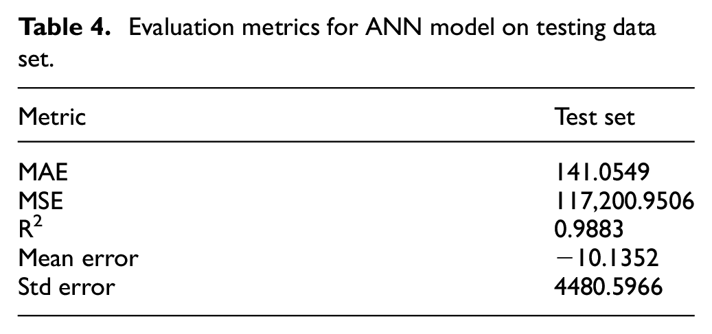
Assuming that the error of the ANN_P model follows a normal distribution, the mean error on the test dataset, which is close to zero (i.e., −10.1352 MPa) indicating the minor bias of this model. It incorporates the standard deviation, std, at 4480.5966 kN, providing the particular distribution of the model error. This low bias is illustrated in Figure 3, with the high density of data points scattered around the 1:1 line. This error is added to the prediction in the MCS, as discussed above.

Figure 3.

Predicted versus experimental data on training and testing dataset of the ANN_P model developed to predict load-bearing capacity of the column p.

MCS with ANN_P model

In this section, the developed ANN trained in the previous section is used for the conventional MCS with the control case which has inputs: µ_D = 442.212 mm; µ_t/D = 0.0811; L = 4000 mm (deterministic); µ_fy = 218.5305; µ_f’c = 10.0336; and all random inputs have the coefficient of variation at 0.1. Given a deterministic axial load, N, which has 15,000 kN applied to the column, a MCS with 10⁶ trials is implemented.

Accounting for the error from ANN model, the mean and standard deviation of column capacity, µ_P and std_P are at 26255.578 kN and 6875 kN, respectively, and thus, the CoV_P is 0.2618. Consequently, the function of P-N has µ_P-N at 11255.578 kN. The standard deviation, std_P-N is equal to the standard deviation of P due to the assumption that the applied load N is deterministic.

Without the error from the ANN model, the std_P and std_P-N is reduced to 4498.643 kN while the corresponding means of P and (P-N) are only higher than those with errors. This is due to the mean error close to zero (i.e., −10.1352 kN), compared to the much larger std_P-N. The standard deviation of error is 4480.5966 which is almost equal to that of (P-N) (i.e., 4498.643 kN). The histogram of (P-N) is given in Figure 4 with an obviously wider variance of data when accounting for the error from the data-driven model. Consequently, the failure probability P_f, which indicates the probability of (P-N) < 0, when errors are included, is higher than when the ANN error is ignored: 0.0497 compared to 0.01539 (shaded in blue), respectively.

Figure 4.

Numeric example of distribution of P-N function, P_f = 0.0497 (with error), 0.01539 (without error).

A parametric study on the effect of inputs’ coefficients of covariance on standard deviation of P is provided in Figure 5, revealing the linear positive correlations between input and interest variables. The trend can also be seen earlier than with µ_P, when fluctuations almost disappeared when n = 10³. Besides, the clear separation of the cases with and without error in the simulation can be observed. For deterministic inputs (CoVs = 0), the randomness of P only relies on the error of ANN model, which is equal to 4480.5966 kN; this is also the starting point for cases with error included. Without such error, the starting point is consistently (0,0). Here, it can be observed that the effect of important inputs such as D or t/D on the std_P based on their corresponding distances to the case where all inputs are random variables. When the inputs that have only a slight effect on the column capacity, P, the angle to the horizontal is smaller, and can be almost zero as in the case of f’_c.

Figure 5.

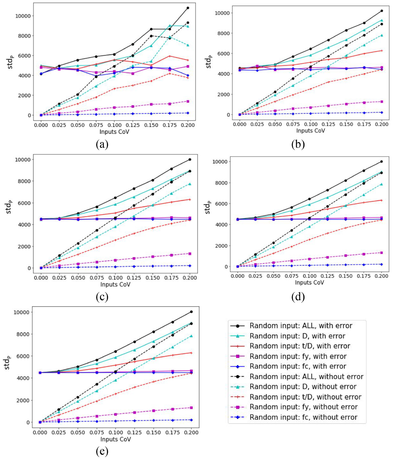
Standard deviation of column capacity versus random inputs CoV with n: (a) 10², (b) 10³, (c) 10⁴, (d) 10⁵, and (e) 10⁶.

The investigation into the critical value for optimization, the failure probability, P_f, is presented in Figure 6. The general trends can be observed with the consistently higher failure probability of MCS with ANN error and the effect of important inputs on the results. The first trend indicates a trade-off between the OF and the uncertainty of the ANN model. The second trend implies the concentration of optimization on the important inputs to obtain the best results. With n = 10⁴, most fluctuations have disappeared, and to reduce the computational effort for the optimization procedure, this value is chosen as the number of trials for analyses in the next section.

Figure 6.

Column failure probability versus random inputs CoV with n: (a) 10², (b) 10³, (c) 10⁴, (d) 10⁵, and (e) 10⁶.

Optimization with MCS and ANN model

The BCMO algorithm is implemented with the control case in the previous section and different threshold for failure probability Pr_max and CoVs of inputs (assumed to be equal). The results of this investigation are provided in Table 5. It is reasonable to observe a consistently higher OF in the case of higher required reliability level (i.e., Pr_max = 0.01). Without the randomness of inputs (inputs’ CoVs are zero), the corresponding OF threshold is 0.0155, compared to that of the counterpart (i.e., Pr_max = 0.05), which is 0.0130. The means of the column capacities are 25,700 kN and 22,587 kN. When the variation of inputs is greatest, CoVs are 0.2, µ_P of Pr_max = 0.01 is 47,035 kN and Pr_max = 0.05 is 36,075 kN.

Table 5.

Optimization results of the numerical example with different input CoVs and threshold for probability of failure.

Pr_max	Inputs CoV	µ_D	µ_t/D	µ_fy	µ_f’c	OF	µ_P	Note
0.01	0.000	447.049	0.07621	217.601	10.507	0.01550	25,700.232	Within boundary
0.01	0.025	412.413	0.09147	213.936	9.357	0.01483	26,156.303	Within boundary
0.01	0.050	440.303	0.08501	214.923	9.677	0.01606	27,342.002	Within boundary
0.01	0.075	464.149	0.08281	214.588	9.620	0.01745	28,492.910	Within boundary
0.01	0.100	515.352	0.08197	213.936	9.353	0.02123	31,489.961	Within boundary
0.01	0.125	530.888	0.08725	214.113	9.403	0.02370	34,815.477	Out-of-boundary
0.01	0.150	635.128	0.07825	213.940	15.420	0.03304	41,755.090	Out-of-boundary
0.01	0.175	682.100	0.08427	213.936	13.237	0.03942	40,877.805	Out-of-boundary
0.01	0.200	715.227	0.08797	232.467	11.321	0.04744	47,035.617	Out-of-boundary
0.05	0.000	393.102	0.08470	218.920	9.935	0.01300	22,587.607	Within boundary
0.05	0.025	406.348	0.08100	213.936	9.499	0.01310	22,701.604	Within boundary
0.05	0.050	437.426	0.07570	213.936	9.486	0.01440	23,898.994	Within boundary
0.05	0.075	414.247	0.08770	213.936	9.353	0.01450	25,692.604	Within boundary
0.05*	0.100	442.212	0.08110	218.531	10.034	0.01590	26,255.578	Within boundary
0.05	0.125	468.390	0.07880	229.160	10.234	0.01824	28,740.219	Out-of-boundary
0.05	0.150	498.830	0.08098	215.147	10.672	0.02006	30,595.504	Out-of-boundary
0.05	0.175	531.898	0.08345	214.837	11.798	0.02356	33,393.695	Out-of-boundary
0.05	0.200	561.456	0.08602	214.797	12.086	0.02694	36,075.563	Out-of-boundary

Case study in Section “MCS with ANNP model.”

The values of µ_P plainly show a positive correlation with the inputs’ CoVs – in other words, the higher the µ_P, the higher the variance of inputs. This is due to the flattening of the probability distribution function or the larger standard deviation of mean of P, the randomness of the inputs increases. For instance, µ_P is 26156.303 kN when input CoVs are 0.025; this value increases to 47035.617 kN with CoVs at 0.2 (Pr_max = 0.01).

It is also seen in Table 5 that µ_D is the variable which changes most, having the tendency to increase, notwithstanding some exceptions. This parameter jumps from 400 mm to 561 mm in the case of Pr_max = 0.05 and to 715 mm when Pr_max = 0.01. Meanwhile, other input parameters can be varied to obtain the best OF such as f’_c, or almost the same, such as t/D and f_y.

For further investigation, different applied loads, N, are chosen (i.e., 10, 15, and 20 MN) along with the variety of input CoVs as given in Figure 7(a), which closely matches the intuition that higher applied load requires more material cost, and thus, has a higher corresponding best OF. For example, with the threshold of Pr_max = 0.01 and input CoVs = 0.2, the best surrogate cost of N = 20,000 kN is 0.05713 compared to that of N = 10,000 kN at 0.03611. Results of the optimization implemented with ANN error are consistently higher than those without it. Again, it is illustrated in Figure 7(a) that higher variance of the input (CoV) leads to the higher requirement of OF. The µ_P in Figure 7(b) shows the tendency to increase with the Pr_max and input CoV with some interesting exceptions where fluctuation occurred.

Figure 7.

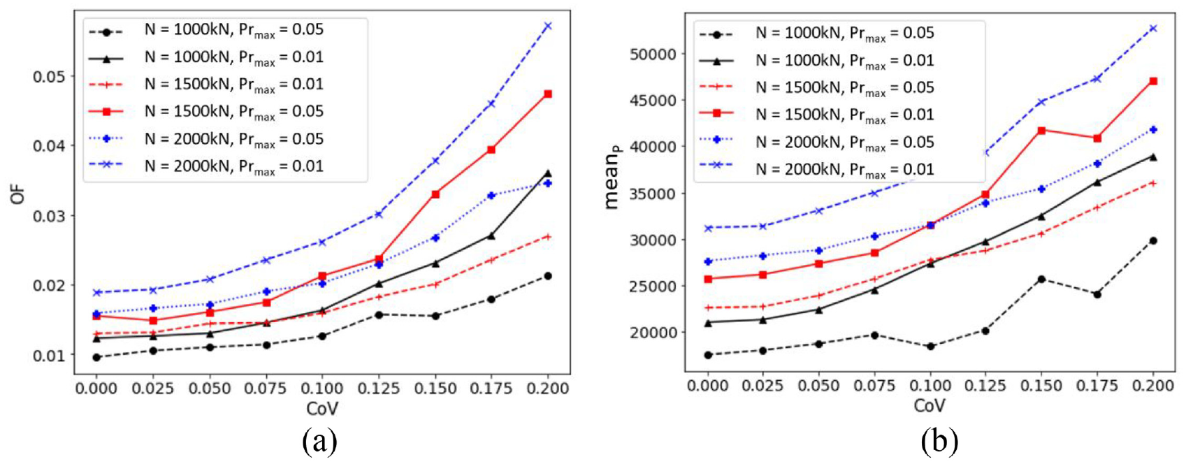
Results of BCMO with MCS and ANN_P with different applied axial loads and input CoVs versus: (a) objective function OF and (b) mean of p, µ_P.

It is worth noting that the analyses in Figure 7 and Table 5 include the out-of-bounds defined in section “Boundaries for design optimization variables” where the maximum CoV is 0.1 and thus out-of-boundary predictions occurred. The maximum µ_P corresponding to CoV = 0.1 is 36,941 kN (with N = 20,000 kN and Pr_max = 0.01). This value is within the range of µ_P [8129, 37915] kN. For instance, the out-of-boundary prediction happened when CoV is larger than 0.1. In the case of N = 20,000 kN and N = 15,000 kN (Pr_max = 0.01, CoV > 0.15), µ_P is larger than 40,000 kN. Even though the main trends are preserved, these results are unpredictable as extrapolations.

Conclusion and outlook

This paper presented a reliability-based investigation for circular CFST members under axial compression. An advanced machine learning method was developed and trained to estimate the axial capacity of the composite elements. The random uncertainties (from both the experimental database and the prediction model) were then incorporated into the prediction machine learning model. The reliability analysis was conducted afterward based on the numerical Monte Carlo technique. The conclusions of this work are listed as follows:

The machine learning prediction model exhibited a considerable ability to predict the axial capacity of CFST columns, with R² up to 0.9883 and MAE = 141.0549 MPa on the testing dataset;

Optimization using the BCMO algorithm was conducted under different failure probability thresholds and coefficient of variation of inputs: the higher the required reliability, the larger the value of the objective function;

Effect of quality of ANN model to the results is also observed by comparison between with/without model error: the uncertainty of data-driven model significantly affects to the output despite of the high accuracy on the evaluation metrics. The weakness of ANN model or machine learning model are revealed in this study: (1) model depend on the boundaries of inputs and outputs to avoid the out-of-boundary effect and (2) reduction of reliability due to this error. Using a less economic column section with higher capacity is the compensation for this uncertainty;

This paper also demonstrated the ability to perform a reliability analysis based on machine learning and global optimization without using specific finite element software.

By combining machine learning and the global optimization technique, the proposed reliability-based procedure can be applied for any structural members (columns and beams).

However, as there are many other factors which might, in practice, affect the structural performance and reliability of a CFST column, future study is needed to address other types of uncertainties: initial imperfections, material properties, structural configurations, and model uncertainties.

Abbreviation and notation

Abbreviation and notation	Detail	Unit
CFST	Circular concrete-filled steel tubular members
ANN	Artificial neural network
MCS	Monte Carlo simulations
BCMO	Balancing composite motion optimization
D	Cross-section outside diameter	mm
t	Wall thickness	mm
t/D	Ratio of wall thickness and outside dimension
L	Length of column	Mm
f_y	Steel yield stress	MPa
f’_c	Concrete cylindrical compression strength	MPa
P	Measured axial capacity	kN
N	Applied axial load	kN
r	Linear statistical correlation coefficient
P_f	Failure probability
OF	Objective function
A_s	Area of steel	mm²
A_c	Area of concrete	mm²
C_steel	Cost of steel
C_concrete	Cost of concrete
P_fmax	Threshold
CoV	Coefficient of variation
µ	Mean
std	Standard deviation
X_oin	Instant global optimization point
P_ANN	Load capacity of the column predicted directly by the ANN model	kN
µ_error,ANN	Mean of error of the prediction
std_error,ANN	standard deviation of error of the prediction
µ_error,test	Mean of error of the prediction on the test dataset
std_error,test	Standard deviation of error of the prediction on the test dataset
UB	Upper bound
LB	Lower bound
P_obp	Out-of-boundary prediction
MAE	Mean absolute error
MSE	Mean squared error
R²	Coefficient of determination

Replication of results

The dataset required to reproduce these findings is appended to this manuscript at https://docs.google.com/spreadsheets/d/1h4S_Vh7t59d8E98AqIYc-2-6T0GI9Djx/edit?usp=sharing&ouid=103283763960933314228&rtpof=true&sd=true.

Footnotes

Appendix A. Histogram of variables

Appendix B. Calculation of linear statistical correlation coefficient

The Pearson linear correlation coefficient r between two real-valued random variables could be calculated based on the following equation⁶⁵:

r = \sqrt{\frac{\sum_{i = 1}^{n} (p_{i} - \bar{p}) (v_{i} - \bar{v})}{\sqrt{\sum_{i = 1}^{n} (p_{i} - \bar{p})^{2}} \sum_{i = 1}^{n} (v_{i} - \bar{v})^{2}}}

where n is the number of the samples, $p_{i}$ and $\bar{p}$ are predicted and mean predicted values, and $v_{i}$ and $\bar{v}$ are measured and mean measured values, respectively. Absolute value of r yields a value between 0 and 1 with 0 means no correlation and 1 means total correlation between two random variables.

Handling Editor: Divyam Semwal

Author contributions

Conceptualization: Hieu Chi Phan, Tien-Thinh Le; Methodology: Hieu Chi Phan, Tien-Thinh Le; Formal analysis and investigation: Huan Thanh Duong; Writing – original draft preparation: Hieu Chi Phan, Tien-Thinh Le, Huan Thanh Duong, Minh Lu Le; Writing – review and editing: Tien-Thinh Le, Minh Lu Le; Supervision: Hieu Chi Phan, Tien-Thinh Le.

Declaration of conflicting interests

The author(s) declared no potential conflicts of interest with respect to the research, authorship, and/or publication of this article.

Funding

The author(s) received no financial support for the research, authorship, and/or publication of this article.

Ethical approval

All procedures performed in studies involving human participants were in accordance with the ethical standards of the institutional and/or national research committee and with the 1964 Helsinki declaration and its later amendments or comparable ethical standards.

Informed consent

Informed consent was obtained from all individual participants included in the study.

Data availability

ORCID iDs

Tien-Thinh Le

Huan Thanh Duong

References

Lai

JCM

. Effect of continuous spirals on uni-axial strength and ductility of CFST columns. J Constr Steel Res 2015; 104: 235–249.

Hossain

KMA

Chu

. Confinement of six different concretes in CFST columns having different shapes and slenderness. Int J Adv Struct Eng 2019; 11: 255–270.

Ding

Fang

Bai

, et al. Mechanical performance of stirrup-confined concrete-filled steel tubular stub columns under axial loading. J Constr Steel Res 2014; 98: 146–157.

Han

L-H

Yao

G-H.

Influence of concrete compaction on the strength of concrete-filled steel RHS columns. J Constr Steel Res 2003; 59: 751–767.

Ali

Nadjai

Goodfellow

Experimental and numerical study on the performance of hollow and concrete-filled elliptical steel columns subjected to severe fire. Fire Mater 2016; 40: 635–652.

Espinos

Gardner

Romero

, et al. Fire behaviour of concrete filled elliptical steel columns. Thin Walled Struct 2011; 49: 239–255.

Bradford

Loh

Slenderness limits for filled circular steel tubes. J Constr Steel Res 2002; 58: 243–252.

Han

L-H

Y-F.

Performance of concrete-encased CFST stub columns under axial compression. J Constr Steel Res 2014; 93: 62–76.

Shi

Y-L

Xian

Wang

W-D

, et al. Mechanical behaviour of circular steel-reinforced concrete-filled steel tubular members under pure bending loads. Structures 2020; 25: 8–23.

10.

Masi

Santarsiero

Mossucca

, et al. Influence of axial load on the seismic behavior of RC beam-column joints with wide beam. Appl Mech Mater 2014; 508: 208–214.

11.

D-Y

Han

L-H

Zhao

X-L.

Seismic performance of the concrete-encased CFST column to RC beam joint: experiment. J Constr Steel Res 2019; 154: 134–148.

12.

Yadav

Chen

Yuan

, et al. Experimental investigation of CFST-RC bridge piers under cyclic loading. Procedia Eng 2017; 173: 1723–1730.

13.

Tran

Nguyen

Dao

, et al. Effect of temperature on the chloride binding capacity of cementitious materials. Mag Concr Res 2021; 73: 771–784.

14.

Chen

Xiong

M-X.

Experimental behavior and design method of rectangular concrete-filled tubular columns using Q460 high-strength steel. Constr Build Mater 2016; 125: 856–872.

15.

Dundu

Compressive strength of circular concrete filled steel tube columns. Thin Walled Struct 2012; 56: 62–70.

16.

Aslani

Tao

, et al. Behaviour and design of composite columns incorporating compact high-strength steel plates. J Constr Steel Res 2015; 107: 94–110.

17.

Zhao

Packer

JA.

Tests and design of concrete-filled elliptical hollow section stub columns. Thin Walled Struct 2009; 47: 617–628.

18.

Mahmoud

Afefy

Kassem

, et al. Strengthening of defected beam–column joints using CFRP. J Adv Res 2014; 5: 67–77.

19.

AISC 360-16. Specification for structural steel buildings ANSI/AISC 360-16. Chicago, IL: American Institute of Steel Construction, 2010.

20.

BS5400-5. Steel, concrete and composite bridges. Code of practice for design of composite bridges. London: British Standards Institute (BSI), 2005.

21.

Eurocode 4. Design of composite steel and concrete structures. Part 1.1, general rules and rules for buildings. London: European Committee for Standardization, British Standards Institution, 2004.

22.

AS/NZS 2327. Composite structures - composite steel-concrete construction in buildings. Barton, Australia: Standards Australia, 2017.

23.

Tran

V-L

Thai

D-K

Kim

S-E.

Application of ANN in predicting ACC of SCFST column. Compos Struct 2019; 228: 111332.

24.

Xiong

M-X

Xiong

D-X

Liew

JYR

. Axial performance of short concrete filled steel tubes with high- and ultra-high- strength materials. Eng Struct 2017; 136: 494–510.

25.

Wang

Z-B

Tao

Han

L-H

, et al. Strength, stiffness and ductility of concrete-filled steel columns under axial compression. Eng Struct 2017; 135: 209–221.

26.

Kuranovas

Goode

Kvedaras

, et al. Load-bearing capacity of concrete-filled steel columns. J Civ Eng Manag 2009; 15: 21–33.

27.

Hatzigeorgiou

Beskos

DE.

Minimum cost design of fibre-reinforced concrete-filled steel tubular columns. J Constr Steel Res 2005; 61: 167–182.

28.

Kalemci

İkizler

Dede

, et al. Design of reinforced concrete cantilever retaining wall using Grey wolf optimization algorithm. Structures 2020; 23: 245–253.

29.

Gandomi

Kashani

Roke

, et al. Optimization of retaining wall design using recent swarm intelligence techniques. Eng Struct 2015; 103: 72–84.

30.

Aydogdu

Cost optimization of reinforced concrete cantilever retaining walls under seismic loading using a biogeography-based optimization algorithm with Levy flights. Eng Optim 2017; 49: 381–400.

31.

Enevoldsen

Sørensen

JD.

Reliability-based optimization in structural engineering. Struct Saf 1994; 15: 169–196.

32.

Pendola

Mohamed

Lemaire

, et al. Combination of finite element and reliability methods in nonlinear fracture mechanics. Reliab Eng Syst Saf 2000; 70: 15–27.

33.

Ahmed

Chateauneuf

Optimal number of tests to achieve and validate product reliability. Reliab Eng Syst Saf 2014; 131: 242–250.

34.

Carvalho

ÉCR

Bernardino

Hallak

, et al. An adaptive penalty scheme to solve constrained structural optimization problems by a craziness based particle swarm optimization. Optim Eng 2017; 18: 693–722.

35.

Vargas

DEC

Lemonge

ACC

Barbosa

HJC

, et al. Differential evolution with the adaptive penalty method for structural multi-objective optimization. Optim Eng 2019; 20: 65–88.

36.

Troian

Uncertainty analysis of structural response under a random impact. Optim Eng 2023; 24: 49–64.

37.

Otero

La Torre

Michailovich

, et al. Optimization of structural similarity in mathematical imaging. Optim Eng 2021; 22: 2367–2401.

38.

Chen

Hou

Zhang

, et al. Reliability-based evaluation for concrete-filled steel tubular (CFST) truss under flexural loading. J Constr Steel Res 2020; 169: 106018.

39.

Neves

Chateauneuf

Venturini

, et al. Reliability analysis of reinforced concrete grids with nonlinear material behavior. Reliab Eng Syst Saf 2006; 91: 735–744.

40.

Liao

F-Y

Han

L-H

S-H.

Behavior of CFST short column and beam with initial concrete imperfection: experiments. J Constr Steel Res 2011; 67: 1922–1935.

41.

Huang

Y-H

Liu

A-R

J-Y

, et al. Experimental investigation of the flexural behavior of CFST trusses with interfacial imperfection. J Constr Steel Res 2017; 137: 52–65.

42.

Chen

Hou

Zhang

, et al. Structural behaviour and reliability of CFST trusses with random initial imperfections. Thin Walled Struct 2019; 143: 106192.

43.

Liao

F-Y

Han

L-H

Tao

Behaviour of CFST stub columns with initial concrete imperfection: analysis and calculations. Thin Walled Struct 2013; 70: 57–69.

44.

Aoues

Chateauneuf

Benchmark study of numerical methods for reliability-based design optimization. Struct Multidisc Optim 2010; 41: 277–294.

45.

Faddoul

Raphael

Chateauneuf

Maintenance optimization of series systems subject to reliability constraints. Reliab Eng Syst Saf 2018; 180: 179–188.

46.

Soares

Mohamed

Venturini

, et al. Reliability analysis of non-linear reinforced concrete frames using the response surface method. Reliab Eng Syst Saf 2002; 75: 1–16.

47.

Kang

W-H

Hicks

, et al. Design resistance evaluation for steel and steel-concrete composite members. J Constr Steel Res 2018; 147: 523–548.

48.

Thai

D-K

Bui

, et al. Gradient tree boosting machine learning on predicting the failure modes of the RC panels under impact loads. Eng Comput 2021; 37: 597–608.

49.

Moon

Kim

Lee

T-H

, et al. Prediction of axial load capacity of stub circular concrete-filled steel tube using fuzzy logic. J Constr Steel Res 2014; 101: 184–191.

50.

Güneyisi

Gültekin

Mermerdaş

Ultimate capacity prediction of axially loaded CFST short columns. Int J Steel Struct 2016; 16: 99–114.

51.

Ahmadi

Naderpour

Kheyroddin

ANN model for predicting the compressive strength of circular steel-confined concrete. Int J Civ Eng 2017; 15: 213–221.

52.

Thanh Duong

Chi Phan

T-T

, et al. Optimization design of rectangular concrete-filled steel tube short columns with Balancing Composite Motion Optimization and data-driven model. Structures 2020; 28: 757–765.

53.

Naser

Thai

H-T.

Evaluating structural response of concrete-filled steel tubular columns through machine learning. J Build Eng 2021; 34: 101888.

54.

Lee

Thai

H-T

, et al. Strength prediction of concrete-filled steel tubular columns using Categorical Gradient Boosting algorithm. Eng Struct 2021; 238: 112109.

55.

Zarringol

Thai

H-T.

Prediction of the load-shortening curve of CFST columns using ANN-based models. J Build Eng 2022; 51: 104279.

56.

Phan

Bui

ND.

Failure assessment of defected pipe under strike-slip fault with data-driven models accounting for the model uncertainty. Neural Comput Appl 2022; 34: 1541–1555.

57.

Phan

Le-Thanh

Nguyen-Xuan

A semi-empirical approach and uncertainty analysis to pipes under hydrogen embrittlement degradation. Int J Hydrogen Energy 2022; 47: 5677–5691.

58.

Phan

Dhar

AS.

Predicting pipeline burst pressures with machine learning models. Int J Press Vessel Pip 2021; 191: 104384.

59.

Thai

H-T

, et al. Concrete-filled steel tubular columns: test database, design and calibration. J Constr Steel Res 2019; 157: 161–181.

60.

Goode

Lam

Concrete-filled steel tube columns-tests compared with Eurocode 4. In: Composite construction in steel and concrete VI, 2011, pp.317–325. Reston, VA: American Society of Civil Engineers.

61.

Denavit Mark

Hajjar Jerome

Perea

, et al. Stability analysis and design of composite structures. J Struct Eng 2016; 142: 04015157.

62.

T-T.

Probabilistic investigation of the effect of stochastic imperfect interfaces in nanocomposites. Mech Mater 2020; 151: 103608.

63.

T-T

Chi Phan

Thanh Duong

, et al. Optimal design of circular concrete-filled steel tubular columns based on a combination of artificial neural network, balancing composite motion algorithm and a large experimental database. Expert Syst Appl 2023; 223: 119940.

64.

Le-Duc

Nguyen

Q-H

Nguyen-Xuan

Balancing composite motion optimization. Inf Sci 2020; 520: 250–270.

65.

Pearson

VII . Note on regression and inheritance in the case of two parents. Proc R Soc Lond 1895; 58: 240–242.

Reliability-based optimization for concrete-filled steel tubular columns incorporating multi-advanced techniques and model constraints

Abstract

Keywords

Introduction

Experimental database and research methodology

Experimental database

Artificial neural network (ANN)

Monte Carlo simulation (MCS)

Optimization with reliability constraint and data-driven model

Balancing composite motion optimization (BCMO)

Uncertainties

Boundaries for design optimization variables

The proposed framework

Results and discussions

The ANNP model

MCS with ANNP model

Optimization with MCS and ANN model

Conclusion and outlook

Abbreviation and notation

Replication of results

Footnotes

Appendix A. Histogram of variables

Appendix B. Calculation of linear statistical correlation coefficient

Author contributions

Declaration of conflicting interests

Funding

Ethical approval

Informed consent

Data availability

ORCID iDs

References

The ANN_P model

MCS with ANN_P model