Condition monitoring of a CNC hobbing cutter using machine learning approach

Abstract

The state of cutting tools profoundly influences the efficiency of the machining processes within the manufacturing industry. Cutting tool faults are highly undesirable and can adversely impact the performance of machine tools, leading to a shortened operational lifespan. Consequently, it is imperative to minimize power consumption by closely monitoring the condition of cutting tools. This necessitates implementing an effective supervision system to continually assess and predict potential faults. In simpler terms, this entails identifying issues that could compromise the lifespan of cutting tools before they escalate into problems like wear, breakage, or complete failure. This proactive approach ensures the optimal and efficient utilization of cutting tools, reduces the need for maintenance and repair, and enhances process stability, among other benefits. In this paper, a novel approach of machine learning for the condition monitoring of hobbing cutters used in Computer Numerical Control Machines (CNCs) was built. Vibration signals from hobbing blades were recorded under various conditions, including healthy and faulty states. The histogram presents a comprehensive overview of the statistical distribution for five variables related to the studied dataset. MATLAB code and scripts are utilized for extracting relevant statistical features, and for identification of the most relevant features, decision tree algorithms were used. For training the ML algorithms the hyperparameters were selected by the Grid Search Method and the Principal component analysis (PCA) was enabled for the reduction of dimensionality and to simplify the data set. The various conditions of hobbing cutters were then classified using tree-based classification models, giving 100% classification accuracy. It helps to develop a novel condition monitoring system for CNC hobbing cutters using machine learning methods to identify problems in hobbing blades. This would ultimately lead to lower power consumption and enhanced performance of machine tools.

Introduction

The precise and automated control offered by CNC machines has revolutionized manufacturing. Hobbing is a vital CNC machining process used to generate gears. It utilizes a hob cutter, a rotary cutting tool with helical teeth that progressively removes material from the workpiece, shaping its teeth. Maintaining the health of the hob cutter is crucial for ensuring consistent gear quality, optimizing production efficiency, and preventing catastrophic failures. ¹ Historically, monitoring tool conditions relied on visual inspection and acoustic emission analysis. While these methods provide a basic understanding of tool wear, they are subjective, prone to human error, and often ineffective in early fault detection. ² The limitations of these methods have motivated the exploration of more objective and reliable techniques. In recent decades, advancements in machine learning (ML) have opened new avenues for intelligent monitoring of CNC processes. Machine learning algorithms can analyse vast amounts of sensor data to identify subtle changes that might escape human observation. This has paved the way for the development of data-driven condition monitoring systems for CNC hobbing machines. Vibration analysis has emerged as a prominent technique for monitoring the health of rotating machinery, including hob cutters. During the hobbing process, the interaction between the cutter and the workpiece generates vibrations that carry valuable information about the tool’s condition. These vibrations can be measured using triaxial accelerometers strategically placed on the machine tool. ³ The concept of using vibration data for hob cutter condition monitoring is not entirely new. Early research focused on developing rule-based systems that employed signal processing techniques to extract features from the vibration signal and correlate them with specific tool wear conditions. ⁴ However, these methods were often limited in their ability to handle complex and non-linear relationships between vibration patterns and tool wear. The emergence of machine learning algorithms has addressed these limitations. Machine learning models can be trained on historical vibration data collected during hobbing operations with healthy and worn cutters. By learning the inherent patterns in the data, these models can effectively distinguish between healthy and faulty tool conditions based on new, real-time vibration measurements. ⁵ The purpose of this research was to develop a machine learning (ML)-based system for the condition monitoring of Computer Numerical Control (CNC) hobbing cutters, which are critical components in the manufacturing industry for gear production. The focus on hobbing cutters is essential because their condition directly affects the quality of the gears produced, the efficiency of the machining process, and the overall operational lifespan of the machine tools. Traditional methods of monitoring tool condition, such as visual inspection and acoustic emission analysis, are subjective and often fail to detect faults early enough to prevent machine downtime and costly repairs. The research aims to address these limitations by implementing a data-driven approach that utilizes vibration signals from the hobbing cutters. These signals, which are rich in information about the tool’s condition, were collected under various operating conditions and analysed using ML algorithms. The goal was to accurately classify the condition of the hobbing cutters in real-time, enabling proactive maintenance measures and contributing to the optimization of machining processes. By employing ML techniques such as decision trees, bagged trees, and logistic regression, the research seeks to identify subtle changes in vibration patterns that indicate tool wear or damage. The system’s ability to predict tool faults before they escalate into major issues leads to significant improvements in process stability, reduced maintenance costs and enhanced productivity. The research also explores the potential of the ML-based condition monitoring system with advanced computing paradigms like cloud platforms and edge computing to further enhance its capabilities and applicability in modern manufacturing environments.

Current developments in tool condition monitoring

Tool Condition Monitoring (TCM) plays a critical role in optimizing machining processes. Traditionally, rule-based systems and human expertise have guided TCM. However, recent advancements in Machine Learning (ML) are revolutionizing this field by offering a data-driven, intelligent approach. ML algorithms excel at extracting patterns from sensor data collected during machining. These sensors monitor parameters like vibration, cutting forces, and acoustic emissions. The data is then used to train ML models to identify different tool wear states, predict tool life remaining, and even prevent catastrophic failures. ⁶ This shift towards data-driven TCM offers several advantages. One key benefit is the ability to handle complex and non-linear relationships between sensor data and tool wear. Unlike rule-based systems that rely on predefined thresholds, ML models can learn these intricate relationships from historical data, leading to more accurate tool condition assessments^7,8 and ML facilitates early detection of tool wear. By analysing subtle changes in sensor data, ML models can identify wear patterns before they become critical, allowing for proactive tool changes and minimizing downtime. ⁹ This predictive capability translates into significant cost savings and improved production efficiency. Several ML algorithms are proving effective in TCM. Convolutional Neural Networks (CNNs) are adept at capturing spatial features from sensor data, enabling them to recognize specific wear patterns. ¹⁰ Recurrent Neural Networks (RNNs), particularly Long Short-Term Memory (LSTM) networks, excel at handling sequential data like sensor readings over time, allowing them to predict future tool wear based on historical trends. ¹¹ The integration of these algorithms is also gaining traction. The research work proposes a hybrid approach combining CNNs and LSTMs for TCM. The CNN identifies the current tool condition, while the LSTM forecasts future wear values, providing a comprehensive picture for informed decision-making. ¹² However, current ML-based TCM approaches face some research gaps. One challenge lies in data acquisition. Gathering high-quality, labelled sensor data from diverse machining processes is crucial for training robust ML models. Collaboration between researchers and industry practitioners can address this by facilitating data collection from real-world manufacturing scenarios. ¹³ Another gap pertains to model interpretability. While ML models excel at prediction, understanding the reasoning behind their decisions is crucial for building trust and ensuring wider adoption. Research into explainable AI (XAI) techniques can help bridge this gap by providing insights into how the models interpret sensor data and arrive at their predictions. ¹⁴ Integrating TCM with cloud-based platforms and edge computing holds immense potential. Cloud platforms offer scalability and centralized data storage, while edge computing enables real-time processing and decision-making at the machine level. ¹⁵ Research into the seamless integration of these technologies can pave the way for truly intelligent and interconnected manufacturing systems. Hence, machine learning is transforming tool condition monitoring. By leveraging its ability to learn from data and identify complex patterns, ML offers a powerful and proactive approach to optimizing machining processes. Addressing data acquisition challenges, developing interpretable models, and integrating with advanced computing paradigms will further propel ML-based TCM toward realizing its full potential in the future of intelligent manufacturing. Even though machine learning shows great promise in tool condition monitoring, there are still some research gaps that need to be addressed. Here are some of the key areas:

• Sensor integration and data quality: Effective TCM relies on high-fidelity sensor data. Research is needed to improve sensor integration strategies and address challenges like sensor noise and data inconsistency.

• Real-time implementation and edge computing: Deploying ML models for real-time monitoring on resource-constrained shop floor environments requires further research on efficient algorithms and edge computing solutions.

• Explainability and interpretability: While ML models can achieve high accuracy, understanding the rationale behind their decisions is crucial for building trust and user acceptance in the industry. More research is needed on developing interpretable models.

• Standardization and generalizability: Current ML-based TCM systems often require extensive training data specific to a particular machining setup. Developing standardized frameworks and transferable models across different manufacturing scenarios remains a challenge.

This study focuses on developing a reliable machine learning (ML) system to monitor the health of hobbing cutters. This approach aims to address current research gaps and improve gear quality, reduce manufacturing costs, and streamline the hobbing process.

Machine learning approach and valuable additions

The methodology in Figure 1, proposes a machine learning system to monitor and predict the health of hobbing cutters. The system analyses vibration data collected from cutters in different conditions (healthy, worn tips/flanks, chipped, cratered, gouged) during operation on a CNC hobbing machine. The study uses a data-driven algorithm in MATLAB to extract key characteristics from the data. Then, a decision tree algorithm identifies the most important features for distinguishing between various cutter conditions. For training the ML algorithms the hyperparameters were selected by Grid Search Method and the Principal component analysis (PCA) was enabled for the reduction of dimensionality and to simplify the data set. Finally, the study compares the effectiveness of five different supervised tree-based algorithms for classifying the health of the hobbing cutters. The valuable contributions of this research are as follows:

• Demonstrating a real-time framework for monitoring hobbing cutter faults in an industrial CNC Hobbing Cutter by combining vibration signal acquisition and machine learning.

• Identifying vibration patterns associated with different stages of the hobbing cutter’s lifespan leads to in-process hobbing cutter defects.

• Developing and training three distinct supervised tree-based algorithms for classifying hobbing cutter faults.

• Predicting tool fault classes using the trained family of tree classifiers and validating the results with a 10-fold cross-validation approach.

Figure 1.

ML approach for predicting hobbing tool health.

The paper’s structure is as follows: Section ‘Experimental setup’ details the experimental setup, input conditions, and vibration signal acquisition. Section ‘Class-wise distribution of data set in histogram’ shows the class-wise distribution of the data set in the histogram. Section ‘Outcomes, discussion and verification using machine learning techniques’ discusses the outcomes, facilitates discussion, and verifies the machine learning-based class prediction. Section ‘Limitations and potential areas for future development’ explores the study’s limitations and potential areas for future development, while final section concludes the paper.

Experimental setup

The signal acquisition experiment was conducted at Laxmi Hydraulics Pvt. Ltd. in Solapur, utilizing a CNC Hobbing Machine (Premier PHA-400). A piezoelectric accelerometer having 10.4 mV/g sensitivity was positioned close to the spindle frame. To capture acceleration signals from the accelerometer, we employed a 16-channel FFT analyser (Dewesoft SIRIUS) as shown in Figure 2. Typically, vibration measurements are obtained near the moving parts of a machine. In this case, during the machining process on the CNC, any parameter variations directly impact the cutting tool first and, consequently, the spindle. Given that the spindle rotates horizontally, the accelerometer’s orientation is aligned vertically, a choice supported by recommendations in the literature. ¹⁶

Figure 2.

Experimental setup.

The details of the experiment are given below:

• Monitoring: Using ‘DewesoftX software’, the vibration data was recorded in real-time (acceleration vs time) during gear hobbing operation.

• Machining conditions: Gears were manufactured on a 20 MnCr5 case-hardened steel blank using an 80mm diameter, 120 mm long HSS hob with a 2.75 mm module. All processes used the same parameters: 6.8 mm depth of cut, 40 rpm spindle speed, and 0.8 mm/min feed rate.

• Test conditions: Five different machining scenarios were performed with the same parameters (depth of cut, feed rate, and speed).

Five conditions of Hobbing cutters are shown in Figure 3, with tip and flank wear being the most common. Over time, this wear can penetrate the tool’s coating and affect the underlying hob material. Furthermore, the hob’s surface may experience the formation of craters, and if these craters grow too large and reach the cutting edge of the hobbing tool, it can lead to the failure of the hobbing tool. Edge chipping may manifest along the tool’s upper edge and sides when the cutting tool material is either too brittle or excessively hard for the particular task. It can also arise from employing a rigid material or experiencing insufficient rigidity and vibrations during the cutting procedure. Another problem tools might confront is the development of built-up edge (BUE), wherein workpiece material accumulates on the cutting tool’s surface. Sometimes, this material deposit can break off, potentially damaging the tool. BUE is a common problem when machining materials like copper alloys, soft steels and aluminium.

Figure 3.

Types of hob faults considered for experimentation. ¹⁷

The wrong type of coolant or insufficient coolant flow and Inadequate cutting clearances on the tool can contribute to BUE formation. Hob failures can arise from various factors aside from normal wear. Chip packing occurs when a significant amount of material is removed, and there needs to be more room or clearance between the teeth to accommodate the chips. This frequently leads to the teeth of the hob breaking away from the main body of the tool within the cutting area, a phenomenon referred to as shelling. Additionally, hob failure can be caused by grinding cracks resulting from the honing process, or it may manifest as microchipping of the tool. ¹⁷ These five conditions are detailed in Table 1 below:

Table 1.

Five conditions of hobbing cutter.

Operations no. Tool conditions	1	2	3	4	5
Healthy	√
Crater wear		√
Tip and flank wear			√
Chipping				√
Gouging					√

Data collection of signals

The requirements for selecting processing parameters in the context of the experiment involve careful consideration of various factors to ensure the accuracy and reliability of the results. The processing parameters, such as the sampling frequency, number of iterations for machine learning algorithms, and hyperparameters for classifiers, play a crucial role in the data collection, feature extraction, and model training processes. Improper selection of these parameters can significantly impact the experiment’s outcomes. For instance, in the signal acquisition process, the sampling frequency is a critical processing parameter. In this experiment, a sampling frequency of 40.5 kHz was chosen to adhere to the Nyquist theorem. ¹⁸ Vibration signals were collected for each of the five operations, and ‘DewesoftX’ software was used to generate the time domain graphs, as depicted in Figure 4. Each action endured for a single second. A machining step was performed to remove imperfections and oxide layers from the workpiece, allowing it to attain a stable condition. Figure 4 demonstrates that the acceleration amplitude and Fast Fourier Transformations (FFT) fluctuations increase with changes in the fault condition.

Figure 4.

Time-domain signals of various types of hob faults. (a) Healthy, (b) crater wear, (c) chipping, (d) tip and flank wear, and (e) gouging.

Correlation between the frequency and amplitude of vibration signals and the formation of various defects in the tool

The signals were acquired from a triaxial accelerometer sensor mounted on the hobbing machine. The signals represent the amplitude of vibration of the hob cutter in the hobbing machine during operation as shown in Figure 4. The following Table 2 shows, a comparison between the peak amplitude and peak frequency of vibration signals for different tool conditions: healthy, crater wear, tip and flank wear, gouging, and chipping.

Table 2.

Comparison between the amplitude and frequency of vibration signals.

Tool condition	Min. peak amplitude (g)	Max. peak amplitude (g)	Peak frequency (Hz)
Healthy (a)	−0.429	0.405	4000
Crater wear (b)	−0.528	0.45	4000
Tip and flank wear (c)	−0.468	0.449	4000
Gouging (d)	−0.475	0.454	4000
Chipping (e)	−0.288	0.316	4000

All the tool conditions listed in the table (healthy and defective) have a peak frequency of around 4000 Hz. This suggests that a frequency around 4000 Hz might be a common characteristic of the vibration signals and not a strong indicator of the presence or absence of defects. The peak amplitude values show more variation between different tool conditions. Healthy tools (a) have a lower range of peak amplitudes (−0.429 to 0.405 g) compared to tools with defects. Tools with defects (b and e) have a wider range of peak amplitudes, with some overlap: Crater wear (b) has a wider range (−0.528 to 0.450 g). Tip and flank wear (c) has a range similar to healthy tools (−0.468 to 0.449 g). Gouging (d) has a range that falls mostly within the range of crater wear (−0.475 to 0.454 g). Chipping (e) has the lowest range (−0.288 to 0.316 g). This suggests that higher amplitudes are indicative of the presence of tool defects, but there are some overlaps between the ranges for different types of defects. To overcome overlaps and to increase the accuracy of classification, in this research work, ML-based techniques were used to develop a condition monitoring system for a CNC Hobbing Cutter.

Additionally, the following observations were made from the graphs:

• The amplitude of the signal increases with the severity of the hobbing cutter condition.

• The signal from a hobbing machine with crater wear has a higher frequency than from a healthy hobbing machine.

• The signal from a hobbing machine with chipping has a higher frequency than from a hobbing machine with crater wear.

• The signal from a hobbing machine with tip flank wear has a higher frequency content than the signal from a healthy hobbing machine, but it is not as high as the frequency content of the signal from a hobbing machine with chipping.

These observations were used to develop condition monitoring algorithms to detect and diagnose hobbing cutter conditions.

Class-wise distribution of data set in histogram

Histograms play a vital role in classifying vibration signals for tool condition monitoring because they offer a concise visualisation of the signal’s amplitude distribution. Here’s how histograms are important:

• Understanding the distribution of vibration amplitudes: A healthy tool will generate vibrations with a distinct amplitude distribution compared to a worn or faulty tool. The histogram reveals this distribution by showing the frequency at which different vibration amplitudes occur.

• Feature extraction for machine learning algorithms: Machine learning algorithms used for classification rely on features extracted from the data. Histograms help extract features like kurtosis, skewness, and standard deviation, which quantify the shape and spread of the vibration amplitude distribution. These features become crucial for the algorithm to differentiate between healthy and faulty tool conditions.

• Identifying anomalies: Deviations from the usual distribution in the histogram can indicate potential problems. For instance, the emergence of a new peak at a higher amplitude might suggest tool wear or bearing faults.

• Simplifying complex data: Vibration signals can be intricate, with multiple frequencies and varying amplitudes. Histograms provide a simplified view of this complexity by focusing on the distribution of amplitudes, making it easier to identify patterns and anomalies.

Hence, histograms are a valuable tool for condition monitoring because they offer a clear understanding of vibration signal distribution and aid in feature extraction for machine learning algorithms. This allows for the effective classification of healthy and faulty tool conditions. Figure 5 shows the class-wise distribution of the data set in the histogram. Here are the comparisons of the Histogram charts:

• Healthy versus crater wear: The histogram for the healthy hobbing cutter shows a normal distribution with a peak around 0. The histogram for the crater wear hobbing cutter shows a right-skewed distribution with a peak around 0.1. This indicates that the crater wear hobbing cutter has more values in the higher range, which is consistent with the fact that crater wear is a more severe condition.

• Healthy versus tip and flank wear: The histogram for the healthy hobbing cutter shows a normal distribution with a peak around 0. The histogram for the tip flank wear hobbing cutter shows a left-skewed distribution with a peak around −0.1. This indicates that the tip and flank wear hobbing cutter has more values in the lower range, which is consistent with the fact that tip and flank wear is less severe than crater wear.

• Healthy versus chipping: The histogram for the healthy hobbing cutter shows a normal distribution with a peak around 0. The histogram for the chipping hobbing cutter shows a bimodal distribution with peaks at −0.2 and 0.2. This indicates that the chipping hobbing cutter has two distinct populations of values, one in the lower range and one in the higher range. This is likely because chipping can cause positive and negative deviations from the mean value.

• Healthy versus gouging: The histogram for the healthy hobbing cutter shows a normal distribution with a peak around 0. The histogram for the gouging hobbing cutter shows a right-skewed distribution with a peak around 0.3. This indicates that the gouging hobbing cutter has more values in the higher range, which is consistent with the fact that gouging is more severe than chipping.

Figure 5.

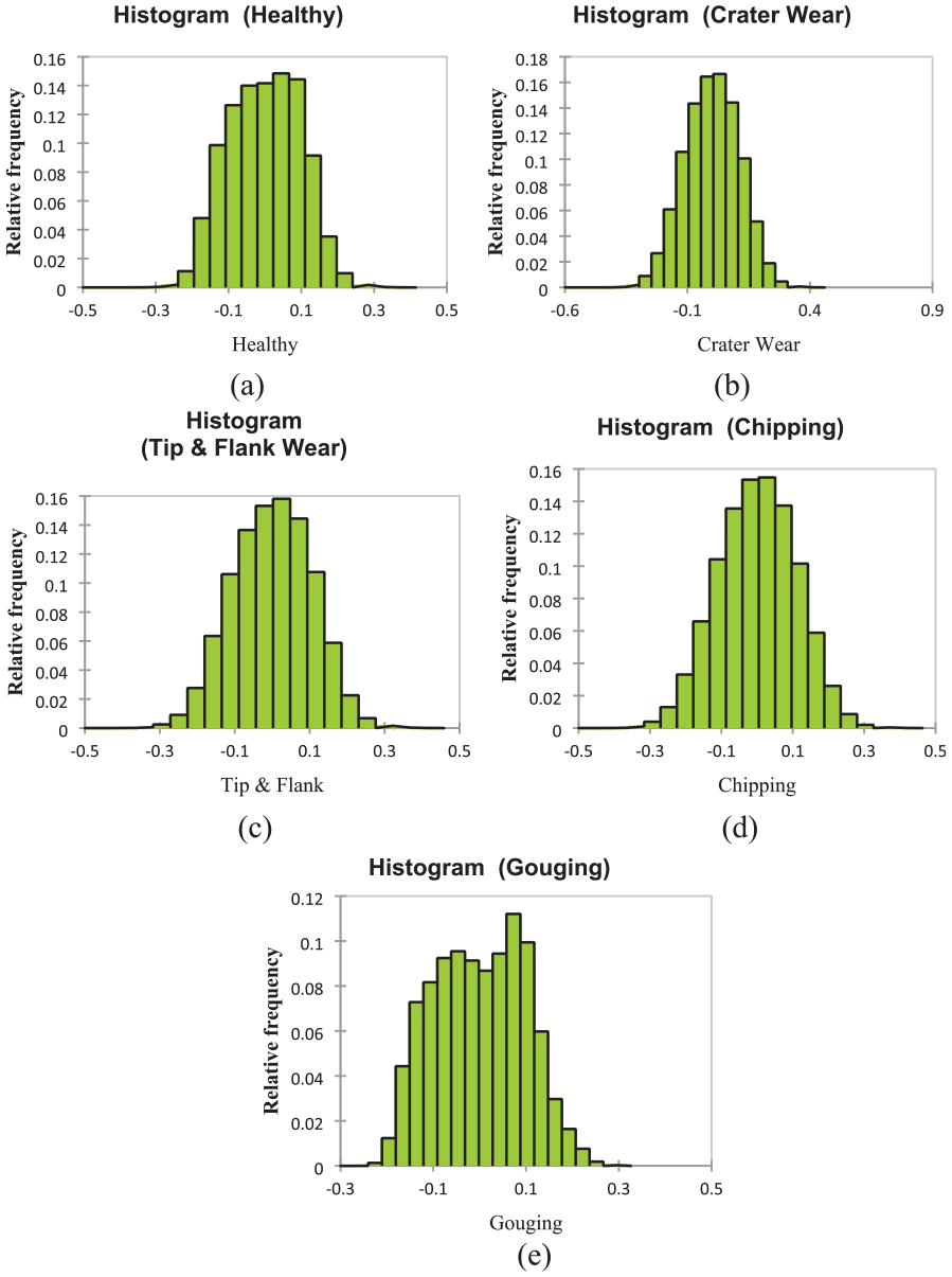
Class-wise distribution of the dataset in a histogram: (a) Healthy, (b) crater wear, (c) tip and flank wear, (d) chipping, and (e) gouging.

The histograms generally show that the healthy hobbing cutter has a normal distribution with a peak around 0. The histograms for the other conditions show different shapes, but they all have peaks that are different from the peak of the healthy hobbing cutter histogram. This indicates that the histograms were used to identify hobbing cutters in different conditions. Table 3 summarises statistics for a histogram of various variables, presumably related to some measurement or data collection. Let us break down the information presented in the table:

• Variables: There are five different variables: ‘Healthy’, ‘Crater Wear’, ‘T and F Wear’, ‘Chipping’, and ‘Gouging’. These variables likely represent different attributes or conditions being measured or observed, as shown in Figure 5.

• No. of Observations: This column shows the total number of observations or data points included in each variable’s analysis. In this case, there are 802,000 observations for each of the five variables.

• Obs. with missing data: This column indicates how many observations for each variable had missing data. There are no missing data points for any variables in this case, as the count is 0.

• Obs. without missing data: This column shows the number of observations that do not have any missing data, which is the same as the total number of observations in this case. Again, there are 802,000 observations with all the data for each variable.

• Min. (Minimum): This column displays the minimum value recorded for each variable. In this case, the ‘Healthy’ variable has a minimum value of −0.429, while the ‘Crater Wear’ variable has a minimum of −0.528.

• Max. (Maximum): This column shows the maximum value recorded for each variable. In this case, the ‘Healthy’ variable has a maximum value of 0.405, while the ‘Crater Wear’ variable has a maximum of 0.45.

• Mean: This column provides the mean or average value for each variable. It represents the central tendency of the data. In this case, the mean value for ‘Healthy’ is approximately −0.001, and for ‘Crater Wear’, it is 0.

• Std. dev. (Standard Deviation): This column displays the standard deviation, a measure of the spread or dispersion of the data. A more minor standard deviation indicates that the data points are closer to the Mean, while a more significant standard deviation suggests more significant variability. In this case, ‘Healthy’ has a standard deviation of 0.098; ‘Crater Wear’ has a standard deviation of 0.11, and so on.

Table 3.

Class-wise summary of statistics of histogram.

Variables	No. of observations	Obs. with missing data	Obs. without missing data	Min.	Max.	Mean	SD
Healthy	802,000	0	802,000	−0.429	0.405	−0.001	0.098
Crater wear	802,000	0	802,000	−0.528	0.45	0	0.11
Tip and flank wear	802,000	0	802,000	−0.468	0.449	0	0.104
Chipping	802,000	0	802,000	−0.475	0.454	0	0.109
Gouging	802,000	0	802,000	−0.288	0.316	0	0.098

These statistics provide an overview of the distribution and characteristics of the data for each of the five variables. They can help to understand the range, central tendency, and variability of the data, which is essential for various analytical and decision-making purposes.

Outcomes, discussion and verification using machine learning techniques

Feature extraction

Time domain features capture unique traits readily observable in the time domain graphs we obtained. To extract statistical attributes from these graphs for various operations, we utilized MATLAB code as described in reference Sanidhya et al. ¹⁹ and employed spreadsheets. We computed a set of 13 statistical characteristics, encompassing metrics such as count, average, standard error, median, mode, variability measures like standard deviation and variance, and statistical properties like kurtosis and skewness. Figure 6(a)–(l) show a graphical representation of variations in Statistical features according to tool conditions. This analysis was performed on a dataset of 500 samples, with 100 samples corresponding to each of the five conditions.

Figure 6.

(a) Variation of ‘Mean’ class wise, (b) variation of ‘STD Error’ class wise, (c) variation of ‘Median’ class wise, (d) variation of ‘Mode’ class wise, (e) variation of ‘Standard Deviation’ class wise, (f) variation of ‘Variance’ class wise, (g) variation of ‘Kurtosis’ class wise, (h) variation of ‘Skewness’ class wise, (i) variation of ‘Range’ class wise, (j) variation of ‘Minimum’ class wise, (k) variation of ‘Maximum’ class wise, (l) variation of ‘Summation’ class wise.

Figure 6(a)–(l) illustrate how different tool setups exhibit variations in their characteristics. Notably, except for the mode, all features show substantial disparities across tool configurations (a) to (e), and these features are deemed the most critical. These results closely align with the outcomes of the Decision Tree algorithm. The study delves into the combinations of these features to identify which sets result in the highest classification accuracy. The order of features recommended by the Decision Tree algorithm is followed to achieve the desired accuracy. Starting with ‘Standard Error and Mean’, additional features are progressively incorporated individually, and their impact on accuracy is evaluated. The highest classification accuracy, reaching 100%, is attained using the minimum number of features, including ‘Standard Error and Mean’. This high level of accuracy remains consistent across all configurations.

Feature selection

It is an essential component of our machine learning approach as it identifies the critical attributes from many options. This procedure trims down the dataset’s complexity, speeds up the classification algorithm, improves classification precision, and makes it easier to interpret the outcomes, as elaborated in reference Sandeep et al. ²⁰ We provided the Decision Tree algorithm with a complete set of 13 features, creating a decision tree structure, as illustrated in Figure 7. Notably, the Decision Tree algorithm identified only two features – namely, mean and standard error as the most significant. Consequently, we exclusively employed these two features for the feature classification task.

Figure 7.

Displays the outcomes of the decision tree of decision tree for feature selection.

The terminology used includes Mean and Standard Error, and a = Healthy, b = Crater Wear, c = Chipping, d = Tip and flank Wear, and e = Gouging, representing various tool conditions.

Feature classification

The process involved utilizing a data mining tool called ‘MATLAB – Classification Learner’. The data used for training the model is 80% (400 samples), and for testing 20% (100 samples). For training the ML algorithms the hyperparameters were selected by Grid Search Method and the Principal component analysis (PCA) was enabled for the reduction of dimensionality and to simplify the data set. Among various classifiers, the tree family classifiers yielded the highest classification accuracy. Therefore, this study primarily compares tree family classifiers to determine the best one. While alternative algorithms such as the K star algorithm, Naïve Bayes, and LWL exist, they are only considered if they offer enhanced classification accuracy. Various methods were employed to categorize different states of hobbing cutter conditions, including tree-based classifiers like Efficient Logistic Regression, Bagged Tree and Decision Tree algorithms. A 10-fold cross-validation approach was used to assess these methods. The Assessment of the classification’s performance is illustrated through a confusion matrix, which offers a detailed breakdown of how various states of the tool conditions were classified.

Decision tree classifier (Model 1)

For training this classifier the hyperparameters selected were Maximum Number of Split (100) and the split criterion (Gini’s diversity index). The experimental findings demonstrate 100% accuracy in classification. Figure 8(a) illustrates the confusion matrix, where the diagonal components of the matrix signify correctly categorized samples, while the diagonal elements indicate samples that were classified incorrectly. Specifically for the Decision Tree classifier, the confusion matrix unveils the following outcomes: In condition ‘a’, 100 samples were accurately labelled as ‘Healthy’, and so forth.

Figure 8.

Displays the classification outcomes achieved using three different algorithms. (a) Decision tree, (b) bagged tree algorithm, and (c) logistic regression.

Bagged tree classifier (Model 2)

For training this classifier the hyperparameters selected were Ensemble Method (Bag), Learner type (Decision tree), Maximum Number of Split (399) and number of learners (30). It produces sets of decision trees and combines them to improve the reliability of predictions. It is a flexible method that accommodates both classification and regression tasks. It introduces additional unpredictability in constructing trees by assessing the most critical features within random subsets instead of choosing them when dividing nodes. This approach results in a more robust model with a classification accuracy of 100%. The confusion matrix (Figure 8 (b)) for Bagged Tree indicates: Under condition ‘a’, 100 samples were correctly classified as ‘Healthy’ and so on.

Logistic regression classifier (Model 3)

For training this classifier the hyperparameters selected were Learner (Logistic Regression), Solver (Auto), and Regularisation (Auto), Regularisation strength: Lambda (Auto), Beta tolerance (0.0001) and multiclass coding (one vs one). This classifier merges the concepts of logistic regression and decision trees, constructing a segmented linear regression model by utilizing linear regression within its terminal nodes. Logistic regression models are constructed at each node using the Logit Boost algorithm. The number of Logit Boost iterations is determined through cross-validation to prevent overfitting. The Logistic Regression classifier achieves a classification accuracy of 100%. The associated confusion matrix Figure 8(c) shows that 100 samples were correctly classified as ‘Healthy’ for ‘condition’ and so on. The data was also validated on unseen data and plotted ROC curve for all three algorithms as shown in Figure 9, Which all the models show an area under the curve (AUC = 1) means 100% accuracy of classification of all conditions in CNC Hobbing Cutter. ²¹

Figure 9.

ROC curves three different algorithms: (a) Decision tree, (b) bagged tree algorithm, and (c) logistic regression.

In the discussion of the results in Table 4 provides an Assessment of different methods employed for classifying features. It is essential to highlight that both the Decision Tree and Bagged Tree algorithms achieve similar levels of accuracy. To be more specific, Table 5 illustrates that the Decision Tree algorithm stands out as the top performer among all the algorithms we tested. Nevertheless, when we consider the practical use of these algorithms for making real-time predictions in the future, the time needed to build the model emerges as a notable issue.

Table 4.

Comparison of performance of different methods employed for classifying features.

Model number	Model type	Status	Accuracy % (validation)	Total cost (validation)	Accuracy % (test)	Total cost (test)
1	Decision tree	Tested	100	0	100	0
2	Bagged tree	Tested	100	0	100	0
3	Logistic regression	Tested	100	0	100	0

Table 5.

Assessment of different methods employed for classifying features.

Type of algorithm Parameter	Bagged tree	Decision tree	Logistic regression	2 classification constrains selected by decision tree
Accuracy (%)	100	100	100	Standard error + mean
Model training time (sec.)	3.91	2.84	4.44

In a direct comparison between Bagged Tree, Decision Tree and Logistic Regression, it becomes evident that Decision Tree is substantially faster in model training, taking only 2.84 s while achieving an accuracy of 100% as shown in Table 4. If accuracy is the sole priority, regardless of time constraints, then Bagged Tree is the best choice. However, if time is a critical factor, one might opt for the Decision Tree algorithm, as it requires the least time among all the options.

Limitations and potential areas for future development

The Hobbing cutter, which utilizes vibration data for hobbing machine health prediction, takes a limited approach to fault prediction. It focuses explicitly on predicting fault categories based on predefined gear hobbing parameters. While the trained model can identify faults within these known categories, its accuracy may vary in real-world situations, especially for unexplored faults. To enhance fault prediction in unforeseen scenarios, conducting further research that considers various parameters for each fault category is vital. Additionally, custom-testing datasets tailored to specific domains are necessary to enable future on-board fault diagnosis and accommodate changes in data distribution. Expanding the dataset would require extensive experimentation, which is beyond the scope of the current study. A recommended approach is to create a versatile deep-learning framework to address this challenge. Furthermore, in cases where the generic model cannot handle unknown faults, human intervention is essential for monitoring and providing feedback. This feedback loop is critical for implementing reinforcement learning techniques.

Conclusion

Effectively showcasing machine learning-driven condition monitoring for a CNC hobbing machine’s hobbing cutter required the collection of vibration signals across different tool conditions. The histogram summary shows that all variables have a consistent number of observations (802,000) and no missing data. The minimum and maximum values for each variable vary, indicating the range of data. The mean and standard deviations provide insights into the central tendencies and spread of the data. The histogram presents a comprehensive overview of the statistical distribution for five variables related to the studied dataset. Statistical features were extracted using MATLAB code and scripts, and the decision tree algorithm was employed to identify important characteristics. Using tree-based classifiers such as Bagged Tree, Decision Tree, and Logistic Regression algorithms, various tool conditions were grouped into categories. Decision Tree emerged as the most efficient classifier when considering the time required for constructing the model and classification accuracy. Although all three classifiers achieved 100% accuracy, time is a more significant parameter for model training. This method is especially well-suited for real-time tool fault detection, leading to decreased power usage within the drive system. The categorized data produced can function as a past benchmark for particular occurrences and can be juxtaposed with present data to forecast the future state of the tool. In the upcoming years, a data fusion method will be included to construct and merge a model to continuously monitor and analyse in real-time.