Sage Journals: Discover world-class research

Abstract

The susceptibility of tools in Computer Numerical Control (CNC) machines makes them the most vulnerable elements in milling processes. The final product quality and the operations safety are directly influenced by the wear condition. To address this issue, the present paper introduces a hybrid approach incorporating feature extraction and optimized machine learning algorithms for tool wear prediction. The approach involves extracting a set of features from time-series signals obtained during the milling processes. These features allow the capture of valuable characteristics relating to the dynamic signal behavior. Subsequently, a feature selection process is proposed, employing Relief and intersection feature ranks. This step automatically identifies and selects the most pertinent features. Finally, an optimized support vector machine for regression (OSVR) is employed to predict the evolution of wear in machining tool cuts. The proposed method’s effectiveness is validated from three milling tool wear experiments. This validation includes comparative results with the Linear Regression (LR), Convolutional Neural Network (CNN), CNN-ResNet50, and Support Vector Regression (SVR) methods.

Keywords

Predictive maintenance CNC machines tool wear monitoring machine learning OSVR

Introduction

Prognostic and health management (PHM) has attracted a considerable amount of attention due to the challenges involved and the development of fault detection, diagnosis and prognosis. Intelligent technologies are applied to solve classification and regression problems with improved recognition and performance. For future machine health prediction, different signal processing, feature extraction, and artificial intelligence (AI) techniques have been developed to ensure human safety and system reliability.^1–4 Degradation in dynamic systems state is a completely normal (inevitable) phenomenon, since such systems operate constantly under severe conditions and in continuous (repetitive) tasks.^5,6 Therefore, a fault presence is a matter of component operating time. The objective in this domain is to monitor the system’s condition (to detect and diagnose any occurring defects) and, more importantly, to track the fault’s evolution for an accurate estimation of the component’s future condition.

In today’s manufacturing systems, tool wear evolution refers to the progressive deterioration and changes that occur in the cutting tool’s condition over time, while performing machining tasks. During the cutting process, the tool is subjected to various mechanical and thermal stresses, leading to material degradation and wear. Initially, tool wear may be minimal, but friction and abrasion progressively wreak havoc as the tool interacts with the workpiece, causing progressive deterioration. As tool wear progresses, cutting edges may become rounded, reducing the machined part’s precision and surface quality. Monitoring and understanding tool wear evolution are crucial in machining operations to optimize tool life, maintain product quality, and enhance process efficiency through timely tool replacements or adjustments. Employing advanced tool materials and coatings, as well as implementing effective cutting strategies, are essential for mitigating the impact of tool wear in modern manufacturing processes. It is therefore necessary to monitor and predict cutting tool wear to avoid component deterioration and rejected products.⁷

Basically, for tool wear monitoring (TWM), three main methods are introduced: physics-based models, data-driven based models and hybrid models. In physics-based models, the physical phenomenon can be expressed in a mathematical degradation model or defects propagation. However, it is very difficult to express a non-linear function which must correspond to a very important system knowledge. In data-driven models, prediction is based on historical data. Such models are widely used, as no detailed knowledge of the monitored components is required. The machines are equipped with sensors and data collection systems that continuously gather information during the machining process. Above all, it generates very satisfactory results with the integration of artificial intelligence (AI) tools as a very powerful learning tool. In hybrid methods, physics and data-based models are implemented to model the tool failure function.^8,9 However, this method requires a deep background knowledge and some models are not upgradeable with online data, which limits their application.¹⁰

In the last decade, researchers have focused on the development of AI techniques, which has led to an increased focus on innovation ideas. Numerous studies have presented new health indicators (HI) for better extraction of monitored components.^11,12 The main problem with these improvement indicators is that their applicability is very limited to certain signals, and it is not possible to generalize this kind of indicator to other signal categories (temperature, acceleration, acoustics, etc.) under high noise background. The TWM process is based primarily on feature extraction, using various advanced signal processing techniques to isolate defects from noise. Several approaches for signal decomposition, including empirical mode decomposition (EMD). EMD decomposes complex data into intrinsic mode functions (IMFs) using a filter that adapts to the signal. Although the summation of these IMFs provides the same information as the original vibration signal but at different frequency levels, EMD has two main drawbacks: mode mixing and inaccuracies in instantaneous values. To address these issues, the improved EMD (EEMD) introduces finite amplitude white noise to the raw signal during decomposition, and this process is repeated with several sets of white noise to obtain averaged IMFs, reducing the risk of mode mixing and improving accuracy.^13–17

The biggest challenge in vibration signal monitoring is the real background noise, often covering fault signatures and making complex signals harder to analyze. Local mean decomposition (LMD) was introduced as an alternative method, decomposing non-stationary signals into product functions (PFs) that consist of signal envelopes and frequency-modulated (FM) signals. Unlike the EMD, LMD requires fewer iterative decompositions and can immediately produce instantaneous frequency modulated (FM) and instantaneous amplitude (AM) without Hilbert transform (HT). However, LMD also shares limitations with EMD, including mode mixing and end effect. To address these issues, researchers proposed the Robust LMD (RLMD), which optimizes the parameter selection process by integrating boundary conditions, envelope approximation, and stopping criteria sifting. Unlike previous studies that focused on individual parameters separately, RLMD employs three algorithms for optimization and uses a heuristic solution to automatically determine the optimal number of sieving iterations in the process.¹⁸ This enhanced approach considers both global and local features of the target signal, aiming to improve the performance of LMD in monitoring complex vibration signals more effectively.^19,20

The major issue with big data for online monitoring lies in efficiently handling the continuous data influx, improving accuracy and reducing the time required for analysis. The integration of signal processing techniques can directly impact the results’ accuracy, especially considering the input signal diversity, such as vibration, current, acoustics, temperature, etc. Therefore, research in this area focuses on the machine learning aspect, in particular on developing and extracting a robust and satisfactory model.^21–23 To address this, researchers concentrate on feature selection and engineering to identify relevant information from the varied input signals.^24,25 Real-time model training is also indispensable for constantly adapting the model as new data appears. Furthermore, the model’s scalability to handle large data sets and its ability to handle data imbalance are key considerations. The research aims to achieve model interpretability, enabling a better understanding and reliability of the model’s predictions.^26,27

Deep Learning (DL) methods have gained prominence in Prognostics and Health Management (PHM),²⁸ including Tool Wear Monitoring (TWM). The research efforts reflect a proactive exploration of DL’s potential, with various studies highlighting advantages, discussing opportunities, and addressing challenges. Rezaeianjouybari et al.²⁹ introduced a DL-based PHM framework, emphasizing its capabilities. As DL evolves, diverse network types are emerging to address the specific PHM requirements. Zhang et al.³⁰ proposed a compact Convolutional Neural Network (CNN) to mitigate overfitting, enhancing model generalizability for fault diagnosis. Wen et al.³¹ utilized a residual CNN for estimating equipment remaining useful life, leveraging residual connections for efficient learning of complex patterns.³² Explores tool condition monitoring in machining, collecting data on cutting force, vibration, and surface texture. Signal processing techniques extract time-domain, frequency domain, and time-frequency features. Gray level processing reveals synchronous changes in surface texture features during cutting tool breakage. Subsequently, an intelligent tool wear prediction model is constructed using support vector regression (SVR), with kernel function parameters optimized through grid search, genetic algorithm, and particle swarm optimization.³³

Cai et al.³⁴ achieved progress in tool condition monitoring through a Stacked Bidirectional Long-Short Term Memory Network (SBiLSTM), effectively capturing temporal dependencies and improving monitoring accuracy, especially for varying conditions. However, as data structures become more complex, a singular network type may prove insufficient. To address this, researchers explore advanced DL architectures, incorporating multiple neural network types and attention mechanisms to handle complex, multidimensional information. Ensembling techniques, combining different network architectures, are also being explored to enhance overall model performance by leveraging individual strengths.

Support Vector Machines (SVM) and Deep Learning (DL) are powerful machine learning techniques, each with distinct advantages. SVM offers training efficiency, simplicity and interpretability making it well suited to small datasets and scenarios in which understanding the model’s decision is crucial. It handles outliers more effectively and requires less data to be efficient. SVM’s explicit feature engineering through kernel functions enhances its capability to capture non-linear relationships.³⁵ On the other hand, DL excels in complex, high-dimensional data, automatically learning intricate patterns without manual feature engineering. It thrives on abundant data and has achieved remarkable success in image recognition, natural language processing, and speech recognition.

Support vector regression (SVR) represents the algorithm’s basic implementation, suitable for simple regression tasks with linearly separable data. It is designed to find an optimal hyperplane within a predefined margin which best fits the training data. However, its performance may be restricted in complex or non-linear regression problems, requiring feature engineering or kernel transformation. The conventional SVR model’s inherent transparency and control require a thorough grasp of the algorithm, allowing for manual fine-tuning of hyperparameters based on domain expertise. However, this method faces challenges in terms of computational intensity, especially when dealing with large datasets or complex kernel functions.³⁶

The Optimized SVR (OSVR) is an advanced version that incorporates various techniques to address those drawbacks and boost performance.³⁷ It includes using different kernels for nonlinear regression, adjusting hyperparameters to improve generalization and utilizing model selection techniques for optimal parameter configuration.³⁸ OSVR implemented capitalizes on efficiency and optimization, harnessing optimized functions for faster training. The automatic hyperparameter tuning streamlines the modelling process, potentially enhancing predictive performance.³⁹ Additionally, it provides a parallel computing support and facilitating preprocessing tasks. OSVR excels in handling non-linear regression tasks and complex datasets, offering enhanced predictive accuracy and robustness.³⁶

Consequently, this paper presents an innovative approach that leverages optimized machine learning algorithms to predict tool wear in machining processes. The proposed method involves several essential stages. First, it extracts a set of features from time-series signals. Next, it integrates an automatic feature selection process, utilizing Relief and intersection feature ranks to automatically select the most relevant features. Finally, an optimized support vector machine is utilized to forecast the wear evolution in cutting tools.

The present manuscript is organized as follows: Section “Mathematical background” introduces the fundamental methodologies encompassing feature extraction, automatic feature selection and OSVM. The proposed method framework is outlined in section “Proposed approach methodology,” followed by the experimental study presentation in section “Experimental setup of CNC machine tool wear.” The proposed method’s application results are presented in section “Results and discussion,” followed by the study’s conclusions in section “Conclusion” and future work in section “Future work.”

Mathematical background

Feature extraction

In signal analysis, scalar feature extraction involves examining the signal to obtain numerical parameters that characterize different aspects of time series signals.⁴⁰ These features serve as essential inputs for a variety of analyses, including fault detection, condition monitoring, and machine learning algorithms. Some scalar features commonly used in vibration signal analysis are listed below⁴¹:

1. Mean: This represents the average value of the vibration signal, providing an indication of its central tendency.

X_{mean} = \frac{1}{n} \sum_{i = 1}^{n} x_{i}

(1)

2. Standard deviation (SD): A measure of the dispersion or spread of the signal values around the mean, offering insights into its variability.

X_{SD} = \sqrt{\frac{1}{n - 1} \sum_{i = 1}^{n} {[x_{i} - \bar{x}]}^{2}}

(2)

3. Skewness (Skw): This feature quantifies the asymmetry of the signal distribution, helping to identify any skewed patterns.

X_{Skw} = \frac{\sum_{i = 1}^{n} {[x_{i} - \bar{x}]}^{3}}{[n - 1] X_{SD}^{3}}

(3)

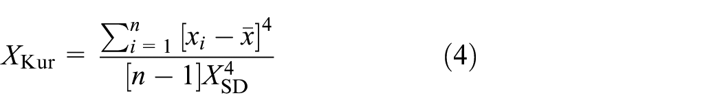
4. Kurtosis (Kur): Describing the shape of the signal compared to a normal distribution, kurtosis indicates whether it is peaked.⁴²

X_{Kur} = \frac{\sum_{i = 1}^{n} {[x_{i} - \bar{x}]}^{4}}{[n - 1] X_{SD}^{4}}

(4)

5. Peak to peak (P2P): P2P indicator is a measure in signal processing that represents the amplitude difference between the maximum positive and maximum negative peaks in a signal or waveform. It provides information about the overall range or magnitude of the signal.

X_{p 2 p} = max (x_{i}) - min (x_{i})

(5)

6. Variance (Var): Variance is the average of the squared differences from the mean of a values set. It quantifies the amount of variability or scatter in the data. A higher variance indicates greater variability in the data which indicates a faulty state in acquired signal.

X \frac{1}{n} \sum_{i = 1}^{n} {(x_{i} - \bar{x})}^{2}

(6)

7. Root Mean Square (RMS): The RMS provides a measure of the effective or root mean square value of a signal, it is particularly useful for quantifying the amplitude of varying signals.

X_{RMS} = \frac{1}{n} \sum_{i = 1}^{n} {(x_{i})}^{2}

(7)

Automatic feature selection

Relief feature selection is a technique used in both classification and regression tasks. It selects relevant features from a dataset by evaluating their importance in distinguishing instances in the feature space. The method involves comparing each instance with its nearest neighbours and computing feature importance scores based on the differences in feature values. The top-k features with the highest scores are then selected for building the predictive model, leading to improved performance and reduced dataset dimensionality.⁴³

A brief overview of relief feature selection is given below:

1. Nearest Neighbor Approach: For each instance in the dataset, Relief compares its feature values with those of its nearest neighbors from the similar target values (for regression). The number of nearest neighbors is a parameter that must be specified using the following equation:

W_{i} = \frac{1}{k} \sum_{j = 1}^{k} | y_{i} - y_{[near - hit] j} | - \frac{1}{l} \sum_{j = 1}^{l} | y_{i} - y_{[near - miss] m} |

(8)

- Where W_i represents the weight assigned to the i-th feature.

- y_i is the target value for the i-th instance.

- y_[near-hit]j is the target value of the j-th instance among the k nearest instances with similar feature values to the i-th instance.

- y_[near-miss]m is the target value of the m-th instance among the l nearest instances with dissimilar feature values to the i-th instance.

2. Feature Importance Scores: Relief computes an importance score for each feature based on the differences between the feature values of the instance and its nearest neighbors. These feature scores indicate how much they correlate with the target variable (regression).

3. Selecting Top Features: Once the importance scores of all the features have been calculated, the top-k features with the highest scores according to fixed threshold (Threshold_rank = 0.5).

In our research, a comprehensive feature selection strategy is used to improve the robustness and generalization capabilities of our predictive models. This approach involves the use of three distinct learning method types (C14, C16, and C46), using various machine learning algorithms or models (Figure 1).

Figure 1.

Feature selection steps.

First, each of these learning methods is applied independently to our dataset. For each method, specific feature selection criteria or techniques are used to identify the most relevant features.

Next, the intersection of the ranking of features selected by the three learning methods is performed. This step allows to isolate the subset of features that are consistently important in the different learning techniques. These selected features are referred to as “stable features” and ensure that the predictive models are based on the most significant and reliable information, thereby enhancing their performance and accuracy. Secondly, this approach is used to avoid the data over-fitting issue, which can affect estimated TWM results.

Optimized support vector regression

The optimization problem described can be solved more easily in its Lagrange dual formulation. The solution to the dual problem provides a lower bound for the solution of the primal problem. However, the optimal values of the primal and dual problems may differ, creating a “duality gap.” In convex problems satisfying a constraint qualification condition, the optimal solution of the primal problem can be determined by solving the dual problem.⁴⁴ To obtain the dual formula (L), a Lagrangian function is constructed from the primal function, introducing nonnegative multipliers for each observation. The goal is then to minimize this dual formula.

\begin{matrix} L (α) = \frac{1}{2} \sum_{i = 1}^{N} \sum_{j = 1}^{N} (α_{i} - α_{i}^{*}) (α_{j} - α_{j}^{*}) {x_{i}}^{'} x_{j} + ε \sum_{i = 1}^{N} (α_{i} + α_{i}^{*}) \\ + \sum_{i = 1}^{N} y_{i} (α_{i}^{*} - α_{i}) \end{matrix}

(9)

In nonlinear SVM regression, the dual formula replaces the inner product of the predictors (x_i, x_j) with the corresponding element of the Gram matrix (g_i, j). The goal of nonlinear SVM regression is to find the coefficients that minimize a certain objective function.⁴⁵

\begin{matrix} L (α) = \frac{1}{2} \sum_{i = 1}^{N} \sum_{j = 1}^{N} (α_{i} - α_{i}^{*}) (α_{j} - α_{j}^{*}) G (x_{i}, x_{j}) \\ + ε \sum_{i = 1}^{N} (α_{i} + α_{i}^{*}) + \sum_{i = 1}^{N} y_{i} (α_{i}^{*} - α_{i}) \end{matrix}

(10)

Subject to

\forall n : 0 \leq a_{n} \leq C, \forall n : 0 \leq a_{n}^{*} \leq C : \sum_{n = 1}^{N} (a_{n} - a_{n}^{*}) = 0

(11)

The function used to predict new values f(x) in nonlinear SVM regression is typically equal to:

f (x) = \sum_{n = 1}^{N} (α_{n} - α_{n}^{*}) G (x_{n}, x) + b

(12)

The minimization problem in nonlinear SVM regression can be expressed in the standard quadratic programming form and solved using common quadratic programming techniques. However, the computational cost can be high, especially when dealing with large Gram matrices that cannot fit into memory. To overcome this, decomposition methods, also known as chunking and working set methods, can be employed.

Decomposition methods involve dividing the observations into two separate sets: the working set and the remaining set. By modifying only the elements within the working set during each iteration, these methods reduce the storage requirements. This is achieved by utilizing only a subset of columns from the Gram matrix in each iteration.

One popular approach for solving SVM problems, including nonlinear SVM regression, is the sequential minimal optimization (SMO) method. SMO performs a series of two-point optimizations. In each iteration, a working set of two points is chosen based on a selection rule that incorporates second-order information. The Lagrange multipliers for this working set are then analytically solved using a specific approach described in Fan et al.^46,47

In SVM regression, the gradient vector (∇L) for the active set is updated after each iteration. The decomposed equation for the gradient vector can be expressed as follows:

{[\forall L]}_{n} = {\begin{matrix} \sum_{i = 1}^{N} (α_{i} - α_{i}^{*}) G (x_{i}, x_{n}) + ε - y_{n}, n \leq N \\ \sum_{i = 1}^{N} (α_{i} - α_{i}^{*}) G (x_{i}, x_{n}) + ε + y_{n}, n > N \end{matrix}

(13)

The iterative single data algorithm (ISDA) is an approach in which one Lagrange multiplier is updated in each iteration.⁴⁸ ISDA is commonly used without the bias term, denoted as b, by incorporating a small positive constant, typically denoted as a, into the kernel function. By omitting the bias term, the constraint related to the sum of Lagrange multipliers is no longer considered.

\sum_{i = 1}^{N} (α_{i} - α_{i}^{*}) = 0

(14)

Each of the solver algorithms iteratively computes until a specific convergence criterion is satisfied. There are several options for convergence criteria, including:

- After each iteration, the software assesses the feasibility gap. If the feasibility gap is found to be smaller than the specified value defined by Gap Tolerance (GT), then the algorithm has satisfied the convergence criterion. At this point, the software returns a solution. The feasibility gap refers to the measure of how close the current solution is to satisfying all constraints and optimality conditions. By comparing the feasibility gap against the GT threshold, the algorithm determines whether the solution has converged adequately.

Δ = \frac{J (β) + L (α)}{J (β) + 1}

(15)

- After each iteration, the software evaluates the gradient vector (∇L). It checks whether the difference in the gradient vector values between the current iteration and the previous iteration is smaller than the specified value defined by delta gradient tolerance (DGT). If this condition is met, the algorithm is considered to have satisfied the convergence criterion, and the software returns a solution. The DGT criterion ensures that the gradient vector has converged sufficiently, indicating that the optimization process has reached a stable point.

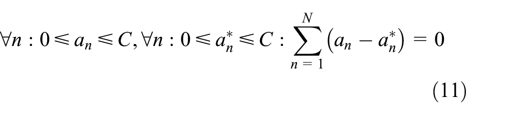
- After each iteration, the software calculates the karush-kuhn-tucker (KKT) violation for all the α_n and $α_{n}^{*}$ values. It checks whether the largest violation among these values is smaller than the specified threshold defined by KKT tolerance. If this condition is met, the algorithm is considered to have satisfied the convergence criterion, and the software returns a solution. The KKT violation measures the extent to which the KKT conditions, which characterize optimality in constrained optimization problems, are violated. By comparing the largest violation against the KKT tolerance threshold, the algorithm determines whether the solution has converged adequately.

Evaluation criteria

Root Mean Square Error (RMSE) and Mean Absolute Error (MAE) are both widely used performance metrics for evaluating regression models in machine learning. They provide a measure of how well the model’s predictions match the actual target values. However, there are some differences between these two metrics⁴⁹:

The RMSE calculates the square root of the average of the squared differences between the predicted values and the actual target values. By squaring the errors before averaging them, RMSE gives higher weight to larger errors, making it more sensitive to outliers compared to MAE. RMSE also has the advantage that it represents the standard deviation of the prediction errors, which is useful for understanding the spread of the errors. However, because of the squaring operation, RMSE penalizes large errors more heavily, which might not be desired in certain applications.

RMSE = \sqrt{\frac{1}{N} \sum_{i = 1}^{N} {(\hat{y} - y)}^{2}}

(16)

MAE measures the average absolute difference between the predicted values and the actual target values. It provides a simple and interpretable metric that directly represents the magnitude of the prediction errors. MAE is less sensitive to outliers since it considers the absolute values of the errors, which means that large errors do not have a disproportionately large impact on the overall metric. However, MAE does not penalize larger errors as strongly as RMSE does, which can be a drawback if you want to give more weight to larger errors.

MAE = \frac{1}{N} \sum_{i = 1}^{N} | \hat{y} - y |

(17)

Where, $\hat{y}$ is the output generated by the model, while $y$ is the target (goal) of input data. N is the length samples data.

Proposed approach methodology

The proposed methodology comprises essentially three parts as shown in Figure 2:

(a) Feature extraction: The initial phase involves the extraction of a diverse features set from time-series signals obtained during milling processes. This meticulous process captures essential characteristics reflecting the dynamic signals behavior. These features serve as crucial input variables for subsequent analyses, providing a nuanced understanding of the underlying patterns in the machining data.

(b) Feature selection: Following feature extraction, a refined feature selection process is introduced. This process is characterized by its meticulous nature and employs Relief and intersection feature ranks (described in section “Automatic feature selection”). By doing so, the approach automatically identifies and prioritizes the most relevant features among the extracted set. This strategic selection ensures that only the most informative features contribute to the subsequent modeling, optimizing the analysis efficiency and effectiveness.

(c) ML regression: The final phase integrates an optimized support vector machine into the machine learning regression framework (described in section “ Optimized support vector regression”). This sophisticated algorithm is specifically tailored to predict the wear evolution in machining tool cuts.

Figure 2.

Diagram of proposed approach.

Experimental setup of CNC machine tool wear

The data set corresponds to a computer numerical control (CNC) cutting tool is introduced in the prognosis and health management (PHM) challenge provided by Simtech Institute in Singapore.⁵⁰ The experimental setup consists of six cutter tools used to cut an identical piece over identical cycle. Total cycles number is equal to 315, in which a cycle represents a single cutting operation of a workpiece (315 cuts). Table 1, shows the detail of CNC cutting tool.

Table 1.

CNC machine tool parameters.

Sampling frequency	50 kHz
Spindle speed	10,400 rpm
Feed speed	1555 mm/min
Radial cutting depth	0.125 mm
Axial cutting depth	0.2 mm

Figure 3 shows the experimental set-up platform. A microscope was used after each cut to measure tool flank wear, and these values are taken as target samples. A tri-component force transducer was installed between the workpiece and the machining table to measure cutting force, while the acceleration and acoustic emission sensors are mounted on the workpiece to collect vibration and acoustic emission signals using a National Instrument (NI) PCI1200 card with a sampling frequency of 50 kHz. The signals collected are then amplified using a Kistler multi-channel load.⁵¹

Figure 3.

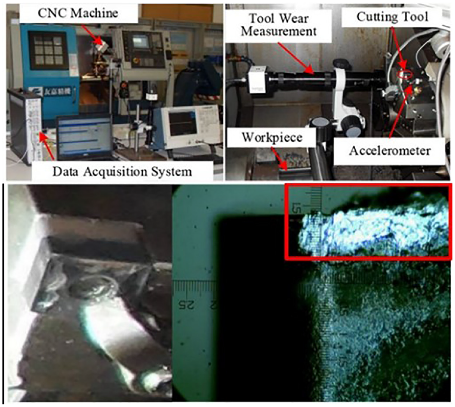
Experimental setup.

The data for a single cut contains the measured wear value for the target and the seven signals collected for the inputs, of which the first three signals are the X, Y and Z dimensions of the force (N), the second three signals X, Y and Z of the vibration (mm/s²) and the last for the acoustic emission (V). Only three out of six milling cutters (C1, C4, and C6) are labelled with a wear measurement.

The wear of each individual flute was assessed through manual inspection utilizing an optical microscope (LEICA MZ12). The elements of CNC machines and tool degradation are presented in the Figure 4.

Figure 4.

(a) The workpeace and cutter and (b) cutter degradation after 315 cuts.⁵¹

In the context of our research, Figure 5 illustrates the process through which experimental data is systematically acquired. This particular illustration provides an overview of the sequential steps and methodologies involved in collecting essential information for our study. Additional information regarding the material of cutters and experimental specifications can be found in reference.⁵²

Figure 5.

Platform of experimental data acquisition.¹⁰

Results and discussion

The tool wear of the three cutters (C1, C4, and C6) are measured from the degraded blade after each cutting operation in three different flutes (Figure 6). The black curve represents the average of the degraded flute wear. The average is used to estimate the overall average wear degradation on any material type. The objective of this study is to avoid incorporating material characteristics into the AI-based prediction model.

Figure 6.

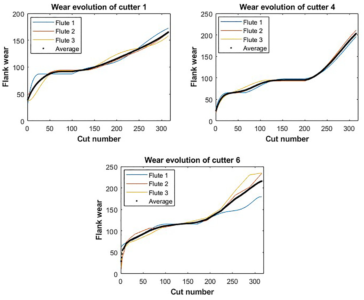
Wear degradation flutes of three cutters.

Figure 7 illustrates wear degradation within the cutting tool process. In this display, the specific values associated with wear degradation are presented as a target, facilitating recognition and understanding within the model framework.

Figure 7.

Averaged wear degradation of three cutters.

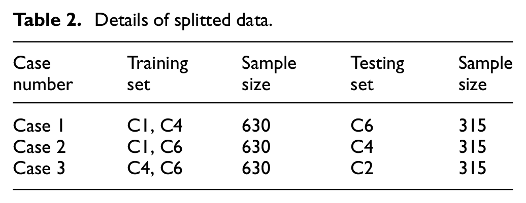
Table 2 provides the data size, with the training set comprising 630 samples from the two cutting machines: C1–C4 for case 1, C1–C6 for case 2 and C4–C6 for case 3. Meanwhile, the test set consists of 315 samples distributed as follows: C6 for case 1, C1 for case 2 and C4 for case 3.

Table 2.

Details of splitted data.

Case number	Training set	Sample size	Testing set	Sample size
Case 1	C1, C4	630	C6	315
Case 2	C1, C6	630	C4	315
Case 3	C4, C6	630	C2	315

A specific feature set is subsequently derived from the first six signals. These features play a crucial role in capturing the distinct characteristics of defect degradation. Using these features, the objective is to closely monitor the evolution and propagation of wear in cutters. This analytical approach allows a comprehensive understanding of wear progress as a function of the cut number, and how it propagates through the machine components.

Figure 8 illustrates a set of features extracted from the input signals of three distinct cutters: C1, C4, and C6. These features, characterized by their monotonic behavior, serve as effective indicators for monitoring wear degradation. Among these indicators, those with the highest correlation with outputs are considered particularly valuable. From the Figure 8, it is clear that the main extracted features exhibit a monotonic trend. The standard deviation (STD) of the initial signal is particularly noticeable, while the other features are unnoticed due to their extremely low values. These values are derived from signals 1 to 6.

Figure 8.

Features of cutters 1, 4, and 6.

The obtained feature matrices consist of three initial matrices, each containing 315 rows and 42 columns, and these matrices are divided between the three scenarios or cases mentioned above. These three matrices are subsequently fused in the feature selection section, in order to select only those features relevant to the prediction of cutter wear degradation. The regression relief function is used to select the optimal features based on the correlated inputs–outputs for each individual case. This is achieved by selecting features that are consistent across the corresponding cases. This selection process is crucial for establishing normalization among the chosen features, guaranteeing uniform representation across all scenarios. This approach allows prioritizing features that demonstrate stability and reliability in distinct scenarios, reinforcing our analysis’s robustness.

The selected features serve as inputs for our optimized vector regression (OSVR), and the wear prediction results are depicted in Figure 9. In this figure, a good prediction can be observed for monitoring the defect evolution and preventing part damage for the three cutters evaluated: C1, C4, and C6. Further insight into the accuracy of these predictions can be gained from the data presented in Figure 10, which presents the associated prediction errors.

Figure 9.

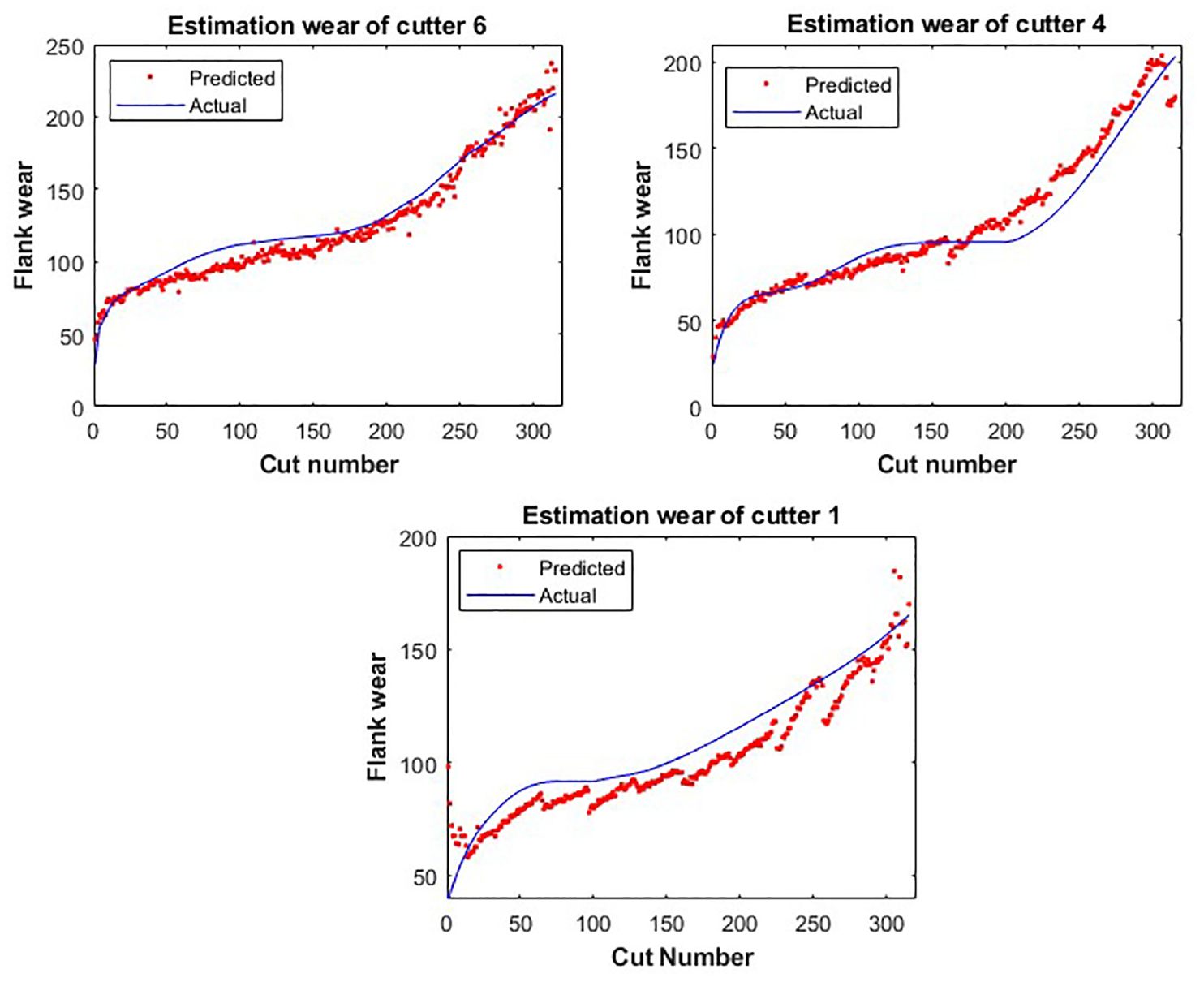
Wear estimation output.

Figure 10.

Prediction errors.

Table 3 provides a comprehensive comparison between our proposed approach to tool wear monitoring and several previous studies.¹⁰ The main objective of this comparison is to evaluate and demonstrate the effectiveness of our new methodology. The PAWO presents the proposed approach results without optimization.

Table 3.

Performance of implemented algorithms.

Model	Experimental results (µm)
	Case 1		Case 2		Case 3
	RMSE	MAE	RMSE	MAE	RMSE	MAE
CNN	22.9	25.3	31.5	24.9	29.4	18.6
LR	19.7	18.0	15.4	13.1	19.1	10.0
PAWO	14.41	11.566	15.12	12.82	16.68	13.795
SVR	12.3	9.3	12.7	10.6	13.3	8.6
ResNet	12.3	10.1	11.7	8.8	13.6	8.9
ResNet-SBILSTM	9.7	7.1	10.9	7.4	14.5	7.4
Proposed methodoly	8.7	7.0	10.1	7.1	10.4	7.3

Table 3 clearly indicates a superior level of performance achieved through the use of the proposed approach. This result considerably reinforces the validity and effectiveness of the steps integrated within our methodology. The obtained results highlight the perfect complementarity of the combined elements and steps, reaffirming the robustness and value of the proposed approach compared to the alternatives presented in the table.

Conclusion

The proposed approach, using optimized machine learning algorithms, is a promising solution for predicting tool wear. The process involves two critical steps: feature extraction and automatic feature selection. Feature extraction involves identifying relevant indicators and characteristics in the machining data that can assess the tool wear evolution. Automatic feature selection based on relief and features intersection for learning ensures that only the most informative features are retained, reducing noise, and improving model accuracy. The optimized support vector machine is used to train the wear tool model by introducing the selected features as inputs. The efficiency of the proposed approach is demonstrated by the results obtained in tool wear estimation, comparing favorably to CNN, LR, SVR, and Resnet-50 with respective values of 8.7, 7.1, and 10.4 for RMSE, and 7.7, 7.1, and 7.3 for MAE. These results ultimately contribute to the enhancement of maintenance decision-making for CNC machines. In overall, this research provides valuable insights into the data-driven approach applied to CNC machining and predictive maintenance applications.

Future work

In this study, the data is constrained due to its limited quantity, and an imbalance in the dataset is observed. To solve this problem, our future work will investigate the influence of unbalanced data on machine learning models and implement strategies to mitigate its impact. In addition, exhaustive data labeling requires considerable human effort and hardware resources. To address this challenge, our plan is to explore both the potential of the proposed approach and transfer learning techniques, which have shown promise in solving such problems.

Furthermore, as part of our methodology, we aim to integrate emission acoustic signals into predictive wear analysis, especially considering their limited utilization in research due to white noise challenges. This integration will leverage cutting-edge signal processing techniques, enhancing the precision and reliability of wear prediction without imposing significant execution time constraints on signal processing tools. By implementing advanced signal processing methodologies, we anticipate a more nuanced and accurate evaluation of wear patterns, thereby contributing to a comprehensive understanding of material degradation over time.

Footnotes

Handling Editor: Chenhui Liang

Declaration of conflicting interests

The author(s) declared no potential conflicts of interest with respect to the research, authorship, and/or publication of this article.

Funding

The author(s) received no financial support for the research, authorship, and/or publication of this article.

ORCID iDs

F Gougam

C Rahmoune

References

Afia

Rahmoune

Benazzouz

, et al. New intelligent gear fault diagnosis method based on Autogram and radial basis function neural network. Adv Mech Eng 2020; 12(5): 1687814020916593.

Afia

Hand

Fawzi

, et al. Gear fault detection, identification and classification using MLP neural network. In: Rao

Khatir

Cuong-Le

(eds.) Recent advances in structural health monitoring and engineering structures: Select proceedings of SHM and ES. Singapore: Springer, 2022, pp. 221–234.

Gougam

Rahmoune

Benazzouz

, et al. Bearing faults classification under various operation modes using time domain features, singular value decomposition, and fuzzy logic system. Adv Mech Eng 2020; 12(10): 1687814020967874.

Afia

Rahmoune

Benazzouz

, et al. New gear fault diagnosis method based on modwpt and neural network for feature extraction and classification. J Test Eval 2021; 49(2): 1064–1085.

Touzout

Benazzouz

Gougam

, et al. Hybridization of time synchronous averaging, singular value decomposition, and adaptive neuro fuzzy inference system for multi-fault bearing diagnosis. Adv Mech Eng 2020; 12(12): 1687814020980569.

Gougam

Chemseddine

Benazzouz

, et al. Fault prognostics of rolling element bearing based on feature extraction and supervised machine learning: application to shaft wind turbine gearbox using vibration signal. Proc Inst Mech Eng C J Mech Eng Sci 2021; 235(20): 5186–5197.

Dimla

. Sensor signals for tool-wear monitoring in metal cutting operations—a review of methods. Int J Mach Tools Manuf 2000; 40(8): 1073–1098.

Wang

Zhao

, et al. Physics guided neural network for machining tool wear prediction. J Manuf Syst 2020; 57: 289–301.

Kong

Chen

. Force-based tool wear estimation for milling process using Gaussian mixture hidden Markov models. Int J Adv Manuf Technol 2017; 92: 2853–2865.

10.

Liu

, et al. Intelligent tool wear monitoring based on parallel residual and stacked bidirectional long short-term memory network. J Manuf Syst 2021; 60: 608–619.

11.

Chen

Song

, et al. A full generalization of the Gini index for bearing condition monitoring. Mech Syst Signal Proc 2023; 188: 109998.

12.

Chen

Zhang

, et al. Power function-based Gini indices: new sparsity measures using power function-based quasi-arithmetic means for bearing condition monitoring. Struct Health Monit 2023; 22(6): 14759217221149745.

13.

Huang

. Ensemble empirical mode decomposition: a noise-assisted data analysis method. Adv Adapt Data Anal 2009; 1(01): 1–41.

14.

Smith

. The local mean decomposition and its application to EEG perception data. J Royal Soc Inter 2005; 2(5): 443–454.

15.

Afia

Gougam

Rahmoune

, et al. Gearbox fault diagnosis using REMD, EO and machine learning classifiers. J Vibr Eng Technol 2023; 1–25.

16.

Afia

Gougam

Rahmoune

, et al. Intelligent fault classification of air compressors using Harris hawks optimization and machine learning algorithms. Trans Inst Measur Control 2023; 46(2): 359–378.

17.

Afia

Gougam

Rahmoune

, et al. Spectral proper orthogonal decomposition and machine learning algorithms for bearing fault diagnosis. J Brazil Soc Mech Sci Eng 2023; 45(10): 1–37.

18.

Aﬁa

Rahmoune

Benazzouz

. An early gear fault diagnosis method based on RLMD, Hilbert transform and cepstrum analysis. Mechatron Sys Control 2020; 49: 115–123.

19.

Liu

Jin

Zuo

, et al. Time-frequency representation based on robust local mean decomposition for multicomponent AM-FM signal analysis. Mech Syst Signal Proc 2017; 95: 468–487.

20.

Jiang

Liu

Peng

, et al. A novel wind speed prediction method based on robust local mean decomposition, group method of data handling and conditional kernel density estimation. Energy Convers Manag 2019; 200: 112099.

21.

Gougam

Afia

Soualhi

, et al. Bearing faults classification using a new approach of signal processing combined with machine learning algorithms. J Braz Soc Mech Sci Eng 2024; 46(2): 65.

22.

Gougam

Rahmoune

Benazzouz

, et al. Health monitoring approach of bearing: application of adaptive neuro fuzzy inference system (ANFIS) for RUL-estimation and autogram analysis for fault-localization. In: 2020 prognostics and health management conference (PHM-Besançon), Besancon, France. Piscataway, NJ: IEEE, 2020, pp. 200–206.

23.

Suthar

Vakharia

Patel

, et al. Detection of compound faults in ball bearings using multiscale-SinGAN, heat transfer search optimization, and extreme learning machine. Machines 2022; 11(1): 29.

24.

Dai

Xiong

, et al. Current sensor fault diagnosis method based on an improved equivalent circuit battery model. Appl Energy 2022; 310: 118588.

25.

Soualhi

Medjaher

Zerhouni

. Bearing health monitoring based on Hilbert–Huang transform, support vector machine, and regression. IEEE Trans Instrum Meas 2014; 64(1): 52–62.

26.

Soualhi

El Koujok

Nguyen

, et al. Adaptive prognostics in a controlled energy conversion process based on long-and short-term predictors. Appl Energy 2021; 283: 116049.

27.

Phate

Bendale

Toney

, et al. Prediction and optimization of tool wear rate during electric discharge machining of Al/Cu/Ni alloy using adaptive neuro-fuzzy inference system. Heliyon 2020; 6(10): e05308.

28.

Vakharia

Shah

Nair

, et al. Estimation of Lithium-ion battery discharge capacity by integrating optimized explainable-AI and stacked LSTM model. Batteries 2023; 9(2): 125.

29.

Rezaeianjouybari

Shang

. Deep learning for prognostics and health management: state of the art, challenges, and opportunities. Measurement 2020; 163: 107929.

30.

Zhang

Chen

Zhang

, et al. A compact convolutional neural network augmented with multiscale feature extraction of acquired monitoring data for mechanical intelligent fault diagnosis. J Manuf Syst 2020; 55: 273–284.

31.

Wen

Dong

Gao

. A new ensemble residual convolutional neural network for remaining useful life estimation. Math Biosci Eng 2019; 16(2): 862–880.

32.

Cheng

Jiao

Shi

, et al. An intelligent prediction model of the tool wear based on machine learning in turning high strength steel. Proc Inst Mech Eng B J Eng Manuf 2020; 234(13): 1580–1597.

33.

Zhang

Han

Luo

, et al. Tool wear monitoring for complex part milling based on deep learning. Appl Sci 2020; 10(19): 6916.

34.

Cai

Zhang

, et al. A hybrid information model based on long short-term memory network for tool condition monitoring. J Intell Manuf 2020; 31: 1497–1510.

35.

Chen

Hao

Guo

, et al. Research on tool wear monitoring in drilling process based on APSO-LS-SVM approach. Int J Adv Manuf Technol 2020; 108: 2091–2101.

36.

Zhang

O’Donnell

. Support vector regression. In: Machine learning. Cambridge, MA: Academic Press, 2020, pp. 123–140.

37.

Cheng

Gai

Jin

, et al. A new method based on a WOA-optimized support vector machine to predict the tool wear. Int J Adv Manuf Technol 2020; 121(9–10): 6439–6452.

38.

Jiang

Liu

, et al. A novel composite electricity demand forecasting framework by data processing and optimized support vector machine. Appl Energy 2020; 260: 114243.

39.

Bera

Lin

Huang

, et al. Establishing a real-time multi-step ahead forecasting model of unbalance fault in a rotor-bearing system. Electronics 2023; 12(2): 312.

40.

Gougam

Rahmoune

Benazzouz

, et al. Bearing fault diagnosis based on feature extraction of empirical wavelet transform (EWT) and fuzzy logic system (FLS) under variable operating conditions. J Vibroeng 2019; 21(6): 1636–1650.

41.

Lei

Zhu

Zhou

, et al. A GAPSO-enhanced extreme learning machine method for tool wear estimation in milling processes based on vibration signals. Int J Prec Eng Manuf Green Technol 2021; 8: 745–759.

42.

Afia

Rahmoune

Benazzouz

. Gear fault diagnosis using Autogram analysis. Adv Mech Eng 2018; 10(12): 1687814018812534.

43.

Urbanowicz

Meeker

La Cava

, et al. Relief-based feature selection: introduction and review. J Biomed Inform 2018; 85: 189–203.

44.

Platt

. Sequential minimal optimization: a fast algorithm for training support vector machines. Technical Report MSR-TR-98–14, 1999.

45.

Vapnik

. The nature of statistical learning theory. New York: Springer, 1995.

46.

Fan

Chen

Lin

. A study on SMO-type decomposition methods for support vector machines. IEEE Trans Neural Netw 2006; 17: 893–908.

47.

Fan

Chen

Lin

. Working set selection using second order information for training support vector machines. J Mach Learn Res 2005; 6: 1871–1918.

48.

Huang

Kecman

Kopriva

. Kernel based algorithms for mining huge data sets: supervised, semi-supervised, and unsupervised learning. New York: Springer, 2006.

49.

Botchkarev

. A new typology design of performance metrics to measure errors in machine learning regression algorithms. Interdiscip J Inform Know Manag 2019; 14: 45–76.

50.

P.d.c. PHM Society, https://www.phmsociety.org/competition/phm/10, (2010, accessed 18 May 2010).

51.

Javed

Gouriveau

, et al. Tool wear monitoring and prognostics challenges: a comparison of connectionist methods toward an adaptive ensemble model. J Intell Manuf 2018; 29: 1873–1890.

52.

Lim

Zhou

, et al. Fuzzy neural network modelling for tool wear estimation in dry milling operation. In: Annual Conference of the PHM Society, San Diego, CA, 27 September–1 October 2009.

Computer numerical control machine tool wear monitoring through a data-driven approach

Abstract

Keywords

Introduction

Mathematical background

Feature extraction

Automatic feature selection

Optimized support vector regression

Evaluation criteria

Proposed approach methodology

Experimental setup of CNC machine tool wear

Results and discussion

Conclusion

Future work

Footnotes

Declaration of conflicting interests

Funding

ORCID iDs

References