Sage Journals: Discover world-class research

Abstract

A modified algorithm is proposed in this study to correct time-varying mesh stiffness (TVMS) and transmission error (TE) in helical gears considering tooth root transition curve. The parametric model of helical gear is established by using the meshing principle of helical gear and hob in order to obtain the accurate tooth root transition curve. Moreover, a TE test rig is set up to compare the theoretical and experimental results. The results of the improved algorithm are very similar to the experimental results compared to the traditional model, and the relative error of TE is also small. In this study, the effect of multi-parameters (e.g. pressure angle, meshing position, transverse contact ratio, and overlap ratio) on TE are investigated by comparing theory with experimental analysis. Through the analysis of parameters, it has been established that an elevation in pressure angle leads to a decrease in TE, followed by an increase. In the event that the meshing position is situated closer to the nodal point, the TE slightly decreases. Moreover, as the transverse contact ratio and overlap ratio increase, the TVMS increases, while the TE decreases. When the overlap ratio approaches an odd multiple of 0.5, the TE displays a significant peak.

Keywords

Tooth root transition curve potential energy method helical gears time-varying mesh stiffness transmission error experimental validation

Introduction

In the gear transmission process, the mesh stiffness of a gear pair varies with the variation of the meshing position, resulting in time-varying mesh stiffness (TVMS). TVMS triggers transmission errors (TE) in the gear pair. In the research on gear system dynamics, TE in gears are a significant cause of vibration and noise in gear transmission systems.¹ Accordingly, investigating the calculation methods and factors of TVMS and TE in gears takes on critical significance in controlling vibration and noise in gear transmission systems.

The calculation methods in terms of TVMS and TE can fall into experimental methods,^2–7 finite element methods (FEM),^8–14 as well as analytical methods.^15–34 In general, experimental methods comprise the use of photoelastic techniques, strain gages, and laser displacement sensors to examine mesh stiffness. Encoders are adopted to examine the rotational angles of gear pairs for calculating TE.^2,3 Pandya and Parey⁴ recently proposed an experimental method based on conventional photoelastic techniques to determine the stress intensity factor (SIF) of cracked gears at different single-tooth contact positions and crack lengths. The relationship between contact position, crack length, crack configuration, SIF, and the overall effective mesh stiffness variation was quantified. Raghuwanshi and Parey⁵ presented an experimental method using strain gages to measure the gear mesh stiffness exhibited by healthy and cracked gear pair systems. They highlighted the significant effect of strain gage placement on the calculation of tooth strain energy. It is noteworthy that gear body deformation is not considered in mesh stiffness measurement in the above-mentioned experimental techniques. Raghuwanshi and Parey⁶ used laser displacement sensors to measure the tooth deflection following the line of action for spur gears, such that the mesh stiffness can be determined. This experimental technique shows the main advantage of measuring the total deflection of gear teeth (e.g. gear body deformation). However, experimental methods require high-precision sensors to minimize measurement errors, which can be costly. Thus, they have been extensively adopted to validate the accuracy of analytical models.

The finite element (FM) method has been widely employed to calculate TVMS and TE. Its advantages lie in its ability to accurately capture the practical gear profiles and consider manufacturing and assembly errors, as well as profile deviations, in the calculation of TVMS and TE. Hedlund and Lehtovaara⁸ utilized linear FE methods to calculate tooth deflection, including the flexibility of tooth bases. The model combines Hertz contact analysis with structural analysis to avoid the demand for large FE meshes. Cooley et al.⁹ compared two FE methods, that is, average slope and local slope, to calculate the mesh stiffness of spur gears. Abruzzo et al.¹⁰ proposed an analytical meshing force equation based on polynomial interpolation using FEM results to precisely simulate contact forces and mesh stiffness in the meshing process. Lin and He¹¹ employed the finite element method to build a gear transmission system model that considers machining errors, assembly errors, and profile deviations. On that basis, static TE can be determined. Although the finite element method can yield highly accurate results when calculating TVMS and TE, it is time-consuming due to the requirement of very small FE elements for the gears. To overcome these limitations, analytical methods and analysis-FEM hybrid methods have been developed. It has been reported that the results obtained from analytical methods are comparable to those from the finite element method but require significantly less computational time.

Wan et al.¹⁵ proposed the cumulative integral potential energy method to obtain the mesh stiffness of helical gears. They further investigated the effect of different parameters (e.g. helix angle and normal modulus) on the mesh stiffness. Tang et al.¹⁶ established single-coupling and double-coupling models to compute the mesh stiffness of helical gear pairs based on the integral potential energy method. Xie et al.¹⁷ proposed an optimized calculation method for filet base stiffness, where two meshing teeth share the same gear body. Based on this, analytical models for mesh stiffness and load distribution were established. The mesh stiffness model introduced a filet base stiffness correction coefficient, enhancing the accuracy of the calculations. Wei et al.¹⁸ examined the effects exerted by tooth tip chamfer and tooth tip relief on the TVMS and dynamic characteristics of helical gear transmission systems. Wan et al.¹⁹ derived a stiffness correction algorithm based on the potential energy method while building a cantilever beam model with non-coincident root circle and base circle for variable cross-sections. Chung et al.²⁰ presented an analytical model considering the involute tooth root curve to calculate the TVMS and loaded static transmission error (LSTE) of helical gear pairs. Based on the slicing method, Yang et al.²² proposed a double-layer iterative calculation method for tooth root stress and load distribution. The coupling relationship between tooth root stress and load distribution along the tooth width distribution and between tooth root stress and load distribution among meshing pairs was separately determined through inner and outer iterations. Yang et al.²³ proposed an optimized tooth tip undercut model and derived the analytical equation for TVMS of undercut teeth. Zheng et al.²⁴ built an analytical-FEM analysis framework combining the centrifugal force field with mesh stiffness and nonlinear dynamics to address high-speed operating conditions. Given the effect of wear evolution, Chen et al.²⁵ derived a TVMS model based on the potential energy method. Dai et al.²⁶ considered gear misalignment and variable load conditions, while Wang and Zhu²⁷ presented an optimized gear mesh stiffness analysis model. An optimized calculation model for the mesh stiffness of helical gear pairs was proposed, which not only considers axial tooth stiffness and axial base stiffness but also considers the effect of surface roughness on transverse tooth stiffness and transverse base stiffness under the conditions of elastic fluid dynamic lubrication. Yang et al.²⁸ put forward a calculation method for TVMS that considers and emphasizes the position of cracks. Chen et al.²⁹ built a gear meshing analysis model comprehensively considering tooth deformation, tooth contact deformation, root deformation, coupling effects of gear body structure, and tooth profile deviations.

Although there have been numerous studies on predicting TVMS and TE, there are still some unresolved issues worth considering.

(1) Conventional TVMS and TE algorithms in research have not accurately considered the root curve of helical gears.

(2) Most literature focuses on studying TVMS and TE in spur gears, while research on helical gears is relatively scarce. However, helical gears are widely used due to their high overlap ratio and low noise, which necessitates thorough research on TVMS and TE in helical gears.

(3) Experimental methods commonly employ techniques such as photoelasticity, strain gages, laser displacement sensors, and encoder to measure TVMS and TE. However, due to the high cost of the experiment, it is often used to verify the accuracy of the analysis model, and is rarely used for parameter impact analysis.

(4) Most studies have only examined the effect of individual parameters, such as the number of teeth, module, and helix angle, on TVMS and TE. However, in gear system design, the center distance and gear ratio generally remain unchanged, while the center distance is influenced by the number of teeth, module, and helix angle. Accordingly, analyzing a single parameter has limited practical engineering significance.

To address these issues, this study proposes an optimized analytical model (IAM) in Chapter 2. The IAM converts the tool tip angle into the tooth root transition curve of the helical gear through meshing equations and coordinate transformations, thereby incorporating it into the calculation of TVMS and TE. In Chapter 3, a gear TE experimental setup is constructed, and high-precision encoders are utilized to measure the rotational angles of the pinion and wheel gears, enabling the calculation of the experimental TE. This experiment serves to compare and validate the improved analytical model. In Chapter 4, the effect of tooth profile shape, meshing position, transverse contact ratio, and overlap ratio on TVMS and TE is analyzed through theoretical and experimental means.

Analytical model

Consideration of tooth root curve in helical gear equations

When gears are machined with a hob, the transition curve of the gear tooth root refers to the trajectory formed through the rolling motion of the tool, as shown in Figure 1.

Figure 1.

Hob generative motion envelope diagram.

The relative coordinate systems between the hob and the gear are illustrated in Figure 2. The translation coordinate system of the hob is denoted as o_h-x_hsy_hsz_hs, where z_hs is consistent with the hob axis. The rotation coordinate system of the hob is o_h-x_hy_hz_h, where z_h coincides with z_hs. The fixed coordinate system of the gear is o-x_sy_sz_s, where z_s is consistent with the gear axis. The rotation coordinate system of the gear is o-x_gy_gz_g, where z_g coincides with z_s.

Figure 2.

Define coordinate system.

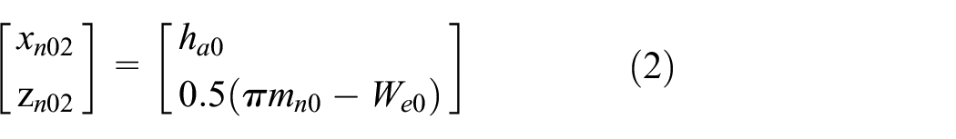
The hob normal plane is presented in Figure 3. The hob’s normal coordinates at points 1, 2, and 3 on the tooth top arc can be obtained based on geometric relationships, as expressed in equations (1)–(3).

[\begin{matrix} x_{n 01} \\ z_{n 01} \end{matrix}] = [\begin{matrix} h_{a 0} \\ 0.5 π m_{n 0} \end{matrix}]

(1)

\begin{matrix} [\begin{matrix} x_{n 02} \\ z_{n 02} \end{matrix}] = [\begin{matrix} h_{a 0} \\ 0.5 (π m_{n 0} - W_{e 0}) \end{matrix}] \end{matrix}

(2)

\begin{matrix} [\begin{matrix} x_{n 03} \\ z_{n 03} \end{matrix}] = [\begin{matrix} h_{a 0} - ρ_{0} (1 - \sin γ_{10}) \\ 0.5 (π m_{n 0} - W_{e 0}) - ρ_{0} \cos γ_{10} \end{matrix}] \end{matrix}

(3)

\begin{matrix} W_{e 0} = S_{n 0} - 2 (h_{a 0} \tan α_{n 0} - \frac{S_{pr}}{\cos α_{n 0}}) \\ - 2 ρ_{0} \tan (\frac{π}{4} - \frac{α_{n 0}}{2}) \end{matrix}

(4)

Figure 3.

Tool normal diagram.

In equations (1)–(4), m_n₀ represents the normal module of the hob, h_a₀ denotes the hob’s tooth top height, S_n₀ corresponds to the hob’s normal tooth thickness, α_n₀ expresses the main blade pressure angle, ρ₀ signifies the tool’s corner radius, Spr is the normal undercut, γ₁₀ is the included angle between the primary cutting edge and the transitional edge.

Hob blade segments are expressed in hob normal section below. The equations for the straight line segment from point 1 to point 2 on the hob blade are given by equation (5).

[\begin{matrix} x_{n 0} \\ z_{no} \end{matrix}] = [\begin{matrix} h_{a 0} \\ l \end{matrix}] 0.5 (π m_{n 0} - W_{e 0}) < l \leq 0.5 π m_{n 0}

(5)

The equations for the curve segment from point 2 to point 3 are represented by equation (6).

[\begin{matrix} x_{n 0} \\ z_{n 0} \end{matrix}] = [\begin{matrix} h_{a 0} - ρ_{0} (1 - \cos \frac{l}{ρ_{0}}) \\ z_{n 02} - ρ_{0} \sin \frac{l}{ρ_{0}} \end{matrix}] 0 \leq \frac{l}{ρ_{0}} < 0.5 π - γ_{10}

(6)

The normal tooth profile equation for any point on the hob tooth top arc is transformed into the end face tooth profile, as shown in equation (7).

{\begin{matrix} x_{0} = x_{n 0} + 0.5 d_{0} \\ y_{0} = y_{n 0} \cos λ_{0} - z_{n 0} \sin λ_{0} \\ z_{0} = y_{n 0} \sin λ_{0} + z_{n 0} \cos λ_{0} \end{matrix}

(7)

Where, λ₀ is the hob lead angle.

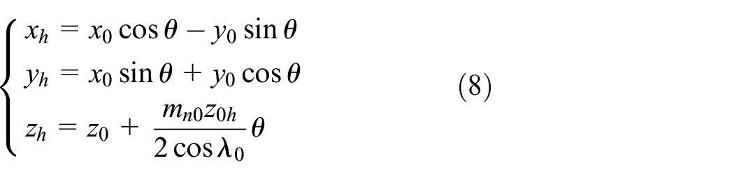
In the hob rotation coordinate system o_h-x_hy_hz_h, the hob’s helical surface is given by equation (8).

{\begin{matrix} x_{h} = x_{0} \cos θ - y_{0} \sin θ \\ y_{h} = x_{0} \sin θ + y_{0} \cos θ \\ z_{h} = z_{0} + \frac{m_{n 0} z_{0 h}}{2 \cos λ_{0}} θ \end{matrix}

(8)

The normal vector of the hob’s helical surface is expressed by equation (9).

{\begin{matrix} n_{xh} = \frac{\partial y_{h}}{\partial l} \frac{\partial z_{h}}{\partial θ} - \frac{\partial z_{h}}{\partial l} \frac{\partial y_{h}}{\partial θ} \\ n_{yh} = \frac{\partial z_{h}}{\partial l} \frac{\partial x_{h}}{\partial θ} - \frac{\partial x_{h}}{\partial l} \frac{\partial z_{h}}{\partial θ} \\ n_{zh} = \frac{\partial x_{h}}{\partial l} \frac{\partial y_{h}}{\partial θ} - \frac{\partial y_{h}}{\partial l} \frac{\partial x_{h}}{\partial θ} \end{matrix}

(9)

The transformation of the hob’s helical surface from the hob rotation coordinate system to the hob translation coordinate system o_h-x_hsy_hsz_hs is shown in equation (10).

[\begin{matrix} x_{hs} \\ y_{hs} \\ z_{hs} \end{matrix}] = [\begin{matrix} x_{h} \cos ϕ_{h} + y_{h} \sin ϕ_{h} \\ - x_{h} \sin ϕ_{h} + y_{h} \cos ϕ_{h} \\ z_{h} \end{matrix}]

(10)

The transformation of the hob’s helical surface from the hob fixed coordinate system to the gear fixed coordinate system o-x_sy_sz_s is described by equation (11).

[\begin{matrix} x_{s} \\ y_{s} \\ z_{s} \end{matrix}] = [\begin{matrix} - x_{hs} \\ - y_{hs} \cos Σ + z_{hs} \sin Σ \\ y_{hs} \sin Σ + z_{hs} \cos Σ \end{matrix}]

(11)

Where, Σ is shaft angle between gear and hob, $Σ = \frac{π}{2} + β - λ_{0}$ , β is gear helical angle.

The angular velocity of the hob in the gear fixed coordinate system is given by equation (12).

{\overset{⇀}{ω}}_{h} = ω_{h} {0, - \sin Σ, - \cos Σ}

(12)

The rotating velocity of the hob in the gear fixed coordinate system is determined by equation (13).

{\overset{⇀}{v}}_{hs 1} = {\overset{⇀}{ω}}_{h} \times {\overset{⇀}{r}}_{hs} = ω_{h} {- y_{hs}, x_{hs} \cos Σ, - x_{hs} \sin Σ}

(13)

The moving velocity of the hob in the gear fixed coordinate system is expressed in equation (14).

{\overset{⇀}{v}}_{hs 0} = \frac{dh}{dt} {0, 0, h}

(14)

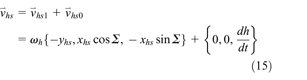
The hob velocity in the gear fixed coordinate system is represented by equation (15).

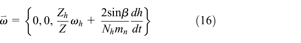
\begin{matrix} {\overset{⇀}{v}}_{hs} = {\overset{⇀}{v}}_{hs 1} + {\overset{⇀}{v}}_{hs 0} \\ = ω_{h} {- y_{hs}, x_{hs} \cos Σ, - x_{hs} \sin Σ} + {0, 0, \frac{dh}{dt}} \end{matrix}

(15)

The angular velocity of the gear is given by equation (16).

\overset{⇀}{ω} = {0, 0, \frac{Z_{h}}{Z} ω_{h} + \frac{2 \sin β}{N_{h} m_{n}} \frac{dh}{dt}}

(16)

The rotating velocity of the gear is determined by equation (17).

{\overset{⇀}{v}}_{gs} = \overset{⇀}{ω} \times {\overset{⇀}{R}}_{s}

(17)

The relative velocity between the hob and the gear is shown in equation (18).

{\overset{⇀}{v}}_{gh} = {\overset{⇀}{v}}_{gs} - {\overset{⇀}{v}}_{hs}

(18)

The transformation of the normal vector of the hob’s helical surface from the hob rotation coordinate system to the hob translation coordinate system is expressed in equation (19).

{\overset{⇀}{N}}_{hs} = [\begin{matrix} n_{xhs} \\ n_{yhs} \\ n_{zhs} \end{matrix}] = [\begin{matrix} n_{xh} \cos ϕ_{h} + n_{yh} \sin ϕ_{h} \\ - n_{xh} \sin ϕ_{h} + n_{yh} \cos ϕ_{h} \\ n_{zh} \end{matrix}]

(19)

The transformation of the normal vector of the hob’s helical surface from the hob translation coordinate system to the gear fixed coordinate system is described by equation (20).

{\overset{⇀}{N}}_{s} = {\begin{matrix} n_{xs} = - n_{xhs} \\ n_{ys} = - n_{yhs} \cos Σ + n_{zhs} \sin Σ \\ n_{zs} = n_{yhs} \sin Σ + n_{zhs} \cos Σ \end{matrix}

(20)

According to the theory of conjugate tooth profiles, to ensure continuous tangent transmission without disengagement or interference, the relative motion velocity vector at the contact point should be perpendicular to the normal vector. The meshing equation between the hob and the gear is given by equation (21).

{\overset{⇀}{N}}_{s} \cdot {\overset{⇀}{v}}_{gh} = 0

(21)

The hob-gear meshing process can be divided into rotational and axial translational movements that do not affect each other. Thus, the meshing equation can be decomposed into rotation and translation equations, as shown in equations (22) and (23).

\begin{matrix} f_{1} = n_{xs} [- \frac{Z_{h}}{Z} y_{s} + y_{hs}] + n_{ys} [\frac{Z_{h}}{Z} x_{s} - x_{hs} \cos Σ] \\ + n_{zs} x_{hs} \sin Σ \\ = n_{xs} [\frac{Z_{h}}{Z} (y_{hs} \cos Σ - z_{hs} \sin Σ) + y_{hs}] \\ + n_{ys} [\frac{Z_{h}}{Z} (- x_{hs}) - x_{hs} \cos Σ] + n_{zs} x_{hs} \sin Σ \\ = 0 \end{matrix}

(22)

\begin{matrix} f_{2} = n_{xs} [\frac{2 \sin β}{Z_{h} m_{n}} y_{s}] + n_{ys} [\frac{2 \sin β}{Z_{h} m_{n}} x_{s}] + n_{zs} \\ = n_{xs} [\frac{2 \sin β}{Z_{h} m_{n}} (y_{hs} \cos Σ - z_{hs} \sin Σ)] \\ + n_{ys} [\frac{2 \sin β}{Z_{h} m_{n}} (- x_{hs})] + n_{zs} \\ = 0 \end{matrix}

(23)

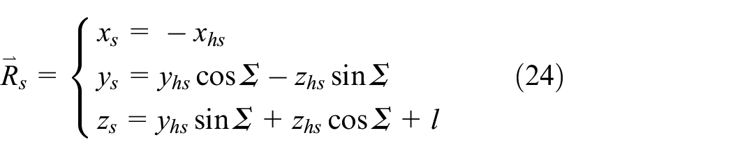
In the machining process, at each instant, the hob’s helical surface and the gear tooth surface involved in the meshing make point contact. The hob cuts the tooth surface at the contact point in each instant. Through the utilization of two distinct meshing equations, denoted as (22) and (23), the parameters of l and θ pertaining to the contact point can be effectively resolved. The transformation of the contact point from the hob translation coordinate system to the gear fixed coordinate system is described by equation (24).

{\overset{⇀}{R}}_{s} = {\begin{matrix} x_{s} = - x_{hs} \\ y_{s} = y_{hs} \cos Σ - z_{hs} \sin Σ \\ z_{s} = y_{hs} \sin Σ + z_{hs} \cos Σ + l \end{matrix}

(24)

The transformation of the contact point from the gear fixed coordinate system to the gear rotation coordinate system is shown in equation (25).

\vec{R} = {\begin{matrix} x_{g} = x_{s} \cos ϕ + y_{s} \sin ϕ \\ y_{g} = - x_{s} \sin ϕ + y_{s} \cos ϕ \\ z_{g} = z_{s} \end{matrix}

(25)

Mesh stiffness of helical gears

The calculation of the contact stiffness per unit tooth width, based on the Hertz theory,¹⁹ is given by equation (26).

k_{h 0} = \frac{π E}{4 (1 - γ^{2})}

(26)

In the equation, E and γ represent the elastic modulus and Poisson’s ratio of the material, respectively.

The calculation of the stiffness corresponding to the foundation stiffness per unit tooth width,¹⁹ is expressed by equation (27).

k_{f 0} (α_{1}) = \frac{E}{\cos^{2} α_{1} {L^{*} {(\frac{u_{f}}{s_{f}})}^{2} + M^{*} (\frac{u_{f}}{s_{f}}) + P^{*} (1 + Q^{*} \tan^{2} α_{1})}}

(27)

In equation (26), L*, M*, P*, Q* and can be expressed using polynomial functions, as shown in equation (28). The values of u_f, s_f, h_fi determined based on the geometric relationship shown in Figure 4, as expressed in equations (29)–(31).

X^{*} = \frac{A_{i}}{θ_{f}^{2}} + B_{i} h_{fi}^{2} + C_{i} \frac{h_{fi}}{θ_{f}} + \frac{D_{i}}{θ_{f}} + E_{i} h_{fi} + F_{i}

(28)

u_{f} = \frac{r_{b}}{\cos α_{1}} - r_{f}

(29)

s_{f} = 2 r_{f} θ_{f}

(30)

h_{fi} = \frac{r_{f}}{r_{int}}

(31)

Figure 4.

Unit tooth width gear matrix stiffness schematic diagram.

In equations (28)–(31), A_i, B_i, C_i, D_i, E_i, F_i are determined based on Table 1. θ_f denotes the root cone angle, r_f expresses the root radius, r_b represents the base circle radius, r_int represents the shaft hole radius, and α₁ is the angle between the direction of force at the contact point and the vertical direction.

Table 1.

Expression (11) coefficient.

	L*	M*	P*	Q*
A_i	$- 5.5740 \times 10^{- 5}$	$6.0111 \times 10^{- 6}$	$- 5.0952 \times 10^{- 6}$	$- 6.2042 \times 10^{- 5}$
B_i	$- 1.9986 \times 10^{- 3}$	$- 2.8100 \times 10^{- 4}$	$1.8550 \times 10^{- 5}$	$9.0889 \times 10^{- 3}$
C_i	$- 2.3015 \times 10^{- 4}$	$- 8.3431 \times 10^{- 5}$	$0.0538 \times 10^{- 4}$	$- 4.0964 \times 10^{- 4}$
D_i	$- 4.7702 \times 10^{- 3}$	$- 9.9256 \times 10^{- 3}$	$- 5.3300 \times 10^{- 4}$	$- 7.8297 \times 10^{- 3}$
E_i	$0.0271$	$0.1624$	$0.2895$	$- 0.1472$
F_i	$6.8045$	$0.9086$	$0.9236$	$0.6904$

As shown in Figure 5, a stiffness calculation coordinate system is established with the tooth center line as the X-axis and the intersection of the base circle and the X-axis as the origin O. The strain energy stored in the gear per unit tooth width is determined using the potential energy method, including the bending strain energy U_b, shear strain energy U_s, and compressive strain energy U_a. The expression for the total strain energy per unit tooth width, consisting of the involute portion and the root portion, is given by equations (32)–(34).

\begin{matrix} U_{b} = \frac{F^{2}}{2 k_{b 0}} = \int_{0}^{x (α_{1})} \frac{{[F_{b} (x (α_{1}) - x) - F_{a} y (α_{1})]}^{2}}{2 E I_{x}} dx \\ + \int_{0}^{X_{1}} \frac{{[F_{b} (x (α_{1}) + x_{1}) - F_{a} y (α_{1})]}^{2}}{2 E I_{x 1}} d x_{1} \end{matrix}

(32)

U_{s} = \frac{F^{2}}{2 k_{s 0}} = \int_{0}^{x (α_{1})} \frac{1.2 F_{b}^{2}}{2 G A_{x}} dx + \int_{0}^{X_{1}} \frac{1.2 F_{b}^{2}}{2 G A_{x 1}} d x_{1}

(33)

U_{a} = \frac{F^{2}}{2 k_{a 0}} = \int_{0}^{x (α_{1})} \frac{F_{a}^{2}}{2 E A_{x}} dx + \int_{0}^{X_{1}} \frac{F_{a}^{2}}{2 E A_{x 1}} d x_{1}

(34)

Figure 5.

Unit tooth width transverse stiffness schematic diagram.

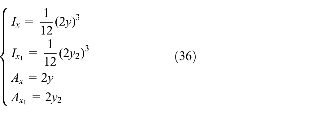
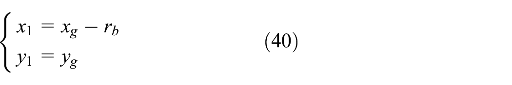
In equations (32)–(34), F represents the force at the contact point; F_a expresses the force component in the x-direction at the contact point; F_b denotes the force component in the y-direction at the contact point, and their expressions are given by equation (35); α₁ is the angle between the force direction at the contact point and the y-axis; G and E represent the shear modulus and elastic modulus, respectively; I_x and A_x denote the sectional moment of inertia and sectional area of the involute portion, while I_x₁ and A_x₁ express the sectional moment of inertia and sectional area of the root portion, and their expressions are given by equation (36). k_b₀, k_s₀, and k_a₀ represent the unit tooth width bending stiffness, unit tooth width shear stiffness, and unit tooth width compressive stiffness, respectively. x(α₁) and y(α₁) represent the coordinates of the contact point, and their expressions are given by equation (37). x and y represent the coordinates of any point on the involute between the starting point and the contact point, and their expressions are given by equation (38). X₁ expresses the horizontal coordinate of the lowest point on the root, and its expression is given by equation (39). x₁ and y₁ denote the transformation of any point on the root from the gear coordinate system o-x_gy_gz_g to the stiffness calculation coordinate system o-xyz; their expressions are expressed in equation (40).

{\begin{matrix} F_{a} = F \sin α_{1} \\ F_{b} = F \cos α_{1} \end{matrix}

(35)

{\begin{matrix} I_{x} = \frac{1}{12} (2 y)^{3} \\ I_{x_{1}} = \frac{1}{12} (2 y_{2})^{3} \\ A_{x} = 2 y \\ A_{x_{1}} = 2 y_{2} \end{matrix}

(36)

{\begin{matrix} x (α_{1}) = r_{b} [\cos α_{1} + (α_{1} + α_{2}) \sin α_{1} - \cos α_{2}] - x_{t} \\ y (α_{1}) = r_{b} [(α_{1} + α_{2}) \cos α_{1} - \sin α_{1}] \end{matrix}

(37)

{\begin{matrix} x = r_{b} [\cos α - (α_{2} - α) \sin α - \cos α_{2}] - x_{t} \\ y = r_{b} [(α_{2} - α) \cos α + \sin α] \end{matrix}

(38)

X_{1} = r_{t} \cos [\arccos (\frac{r_{b}}{r_{t}}) - α_{t}] - r_{f} \cos α_{2}

(39)

{\begin{matrix} x_{1} = x_{g} - r_{b} \\ y_{1} = y_{g} \end{matrix}

(40)

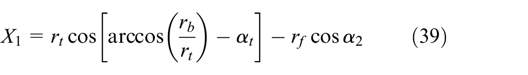
In equations (35)–(40), r_b is the base circle radius, r_f is the root circle radius, r_t is the starting point radius of the involute, α₁ is the angle between the force direction at the contact point and the y-axis, α₂ is the half angle of the root tooth thickness, α_t is the angle between the starting point of the involute and the Y-axis, x_t is the coordinates of the starting point on the involute in the stiffness calculation coordinate system o-xyz and its expression is given by equation (41).

x_{t} = r_{b} [\cos α_{t} + (α_{t} + α_{2}) \sin α_{t} - \cos α_{2}]

(41)

α_{t} = a_{k} + ξ_{M (0)} - \tan a_{k} - \frac{π}{2 z}

(42)

where a_k is the pressure angle at the pitch circle, ξ_M₍₀₎ is the helix angle at the starting point of the involute.

By substituting equations (35)–(42) into equations (32)–(34), the expressions for unit tooth width bending stiffness, unit tooth width shear stiffness, and unit tooth width compressive stiffness are obtained, as given by equations (43)–(45).

\begin{array}{l} k_{b 0} (α_{1}) = 1 / (\int_{- α_{1}}^{- α_{t}} \frac{3 (α_{2} - α) \cos α}{2 E [\sin α + (α_{2} - α) \cos α]} \times \\ {1 + \cos α_{1} [(α_{2} - α) \sin α - \cos α]}^{2} d α \\ + \int_{0}^{X_{1}} \frac{3 {[x (α_{1}) + x_{1}] \cos α_{1} - y (α_{1}) \sin α_{1}}^{2}}{2 E h_{x 1}^{3}} d x_{1}) \end{array}

(43)

\begin{matrix} k_{s 0} (α_{1}) = 1 / (\int_{- α_{1}}^{- α_{t}} \frac{1.2 (1 + γ) (α_{2} - α) \cos α \cos^{2} α_{1}}{G [\sin α + (α_{2} - α) \cos α]} d α \\ + \int_{0}^{X_{1}} \frac{1.2 \cos^{2} α_{1}}{G A_{x 1}} d x_{1}) \end{matrix}

(44)

\begin{matrix} k_{a 0} (α_{1}) = 1 / (\int_{- α_{1}}^{- α_{t}} \frac{(α_{2} - α) \cos α \sin^{2} α_{1}}{E [\sin α + (α_{2} - α) \cos α]} d α \\ + \int_{0}^{X_{1}} \frac{\sin^{2} α_{1}}{E A_{x 1}} d x_{1}) \end{matrix}

(45)

The angle between the contact point and the x-axis, α₁ is transformed into the chordal length of the contact point m, and its expression is given by equation (46).

m = r_{b} (α_{1} + \tan a + \frac{π}{2 Z} - a)

(46)

Where Z is the number of teeth on the gear, a is the pressure angle at the pitch circle.

The meshing process of helical gears is different from that of spur gears, as shown in Figure 6. When viewed from the end face, it can be considered as a spur gear. A tooth enters the meshing at point A and exits at point B. Within the meshing region, due to the presence of the helix angle, the contact line of a single tooth first increases and then decreases. The meshing stiffness of a single tooth also increases and then decreases in the meshing process. According to the principle of sectional integration, the contact length AB on the end face is divided into N segments, each with a length Δx, as expressed in equation (47).

Δ x = \frac{ε_{α} p_{bt}}{N}

(47)

Where ε_α is the transverse contact ratio, and p_bt is the base pitch.

Figure 6.

Helical gear meshing process.

The tooth width on the meshing surface is represented by the side length AC, and each segment has a length Δy, as expressed in equation (48).

Δ y = \frac{ε_{α} p_{bt}}{N \tan β_{b}}

(48)

Where β_b is the helix angle of the base circle.

The expression for the length of the contact line of a single tooth can be discussed in two cases, as shown in Figure 7. When the transverse contact ratio is smaller than the overlap ratio, that is, ε_α < ε_β, the range of the single tooth contact line from the starting position A to point B is given by equation (49).

k_{x} (m_{A} + m) = \sum_{i = 0}^{m} Δ y * k_{x 0} (m_{A} + Δ x * i)

(49)

Figure 7.

Contact length of single gear: (a) $ε_{α} < ε_{β}$ and (b) $ε_{α} > ε_{β}$ .

Where m_A is the chordal length of the contact line at point A, and the range of the contact line from the starting position A to point B is expressed as 0 ≤ m < N. k_x(m) denotes the single tooth contact stiffness k_h(m), the single tooth foundation stiffness k_f(m), the single tooth bending stiffness k_b(m), the single tooth shear stiffness, k_s(m) and the single tooth compressive stiffness k_a(m). k_x₀(m) is the unit tooth width contact stiffness k_h₀(m), the unit tooth width foundation stiffness k_f₀(m), the unit tooth width bending stiffness k_b₀(m), the unit tooth width shear stiffness k_s₀(m), and is the unit tooth width compressive stiffness k_a₀(m).

When the position of the single tooth contact line passes through point B, the single tooth stiffness G is given by equation (50).

G = \sum_{i = 0}^{N} Δ y * k_{x 0} (m_{A} + Δ x * i)

(50)

The range of the single tooth contact line from point B to point C is given by equation (51).

k_{x} (m_{A} + m) = G

(51)

where the range of the contact line from point B to point C is N ≤ m < M, and $M = \frac{ε_{β} * p_{bt}}{Δ x}$ .

The range of the single tooth contact line from point C to point D is given by equation (52).

k_{x} (m_{A} + m) = G - \sum_{i = 0}^{m - M} Δ y * k_{x 0} (m_{A} + Δ x * i)

(52)

where the range of the contact line from point C to point D is $M \leq m < \frac{(ε_{α} + ε_{β}) * p_{bt}}{Δ x}$ and $M = \frac{ε_{β} * p_{bt}}{Δ x}$ .

When the transverse contact ratio is greater than the overlap ratio, that is, ε_α > ε_β, the range of the single tooth contact line from the starting position A to point C is given by equation (53).

k_{x} (m_{A} + m) = \sum_{i = 0}^{m} Δ y * k_{x 0} (m_{A} + Δ x * i)

(53)

where the range of the contact line from the starting position A to point C is 0 ≤ m < M’ and $M^{'} = \frac{b * \tan β_{b}}{Δ x}$ .

When the position of the single tooth contact line passes through point C, the single tooth stiffness G’ is given by equation (54).

G^{'} = \sum_{i = 0}^{M^{'}} Δ y * k_{x 0} (m_{A} + Δ x * i)

(54)

The range of the single tooth contact line from point C to point B is written in equation (55)

\begin{matrix} k_{x} (m_{A} + m) = G^{'} + \sum_{i = M^{'}}^{m} Δ y * k_{x 0} (m_{A} + Δ x * i) \\ - \sum_{i = 0}^{m - M^{'}} Δ y * k_{x 0} (m_{A} + Δ x * i) \end{matrix}

(55)

where the range of the contact line from point C to point B is expressed as M’ ≤ m < N, and $M^{'} = \frac{b * \tan β_{b}}{Δ x}$ .

When the position of the single tooth contact line passes through point B, the single tooth stiffness H is expressed in equation (56).

\begin{matrix} H = G^{'} + \sum_{i = M^{'}}^{N} Δ y * k_{x 0} (m_{A} + Δ x * i) \\ - \sum_{i = 0}^{N - M^{'}} Δ y * k_{x 0} (m_{A} + Δ x * i) \end{matrix}

(56)

The range of the single tooth contact line from point B to point D is written in equation (57).

k_{x} (m_{A} + m) = H - \sum_{i = 0}^{m - N} Δ y * k_{x 0} (m_{A} + Δ x * i)

(57)

where the range of the contact line from point B to point D is $N \leq m < \frac{(ε_{α} + ε_{β}) * p_{bt}}{Δ x}$ .

The meshing stiffness of a single gear pair k_s(m) is obtained based on the series-parallel theory, as given by equation (58).

k_{s} (m_{A} + m) = \frac{1}{\frac{1}{k_{x 1} (m_{A} + m)} + \frac{1}{k_{x 2} (m_{A} + m)}}

(58)

where 1 and 2 denote the pinion gear and wheel gear, respectively.

The comprehensive meshing stiffness of a helical gear pair is obtained by translating the meshing stiffness of a single gear pair Z base pitches and then superimposing them, as written in equation (59).

k_{c} (m_{A} + m) = \sum_{n = 0}^{Z - 1} k_{s} (m_{A} + m + n * p_{bt})

(59)

where n is the nth tooth of the gear; Z denotes the number of teeth; k_s expresses the meshing stiffness of a single helical gear pair; p_bt is the base pitch; k_c is the comprehensive meshing stiffness of the helical gear pair.

Transmission error of helical gear pairs

Given the transmission system without the effects of transmission shafts, bearings, and housing elastic deformation, the gear system can be simplified as a time-varying spring system following the line of contact; an equivalent dynamic model is illustrated in Figure 8.

Figure 8.

Dynamic model of helical gear pair.

The dynamic equation of the gear pair is expressed in equation (60):

m \overset{\cdot\cdot}{x} + c \overset{\cdot}{x} + k_{c} x = W

(60)

Where x represents the relative displacement following the line of contact between the two gears; c denotes the damping coefficient of the gear pair; k_c expresses the comprehensive meshing stiffness of the helical gear pair; W is the equivalent load.

The equivalent load W is expressed in equation (61):

W = \frac{T_{1}}{r_{b 1}} = \frac{T_{2}}{r_{b 2}}

(61)

Where T₁ and T₂ denote the torques applied to the pinion and wheel gears, respectively; r_b₁ and r_b₂ represent the radii of the base circles of the pinion and wheel gears, respectively.

With the dynamic terms (inertial force and damping force) neglected, the TE can be obtained, as expressed in equation (62):

TE = \frac{T_{1}}{r_{b 1} * k_{c}}

(62)

As revealed by equation (61), a higher average value of the comprehensive meshing stiffness in a helical gear pair leads to a stronger resistance against deformation under loads. Since new energy vehicles have been more extensively employed, the torque range experienced by gearbox gears expands continuously. Higher average meshing stiffness results in reduced deformation of gears under higher torque loads, such that they are enabled to accommodate a wider range of torque. Moreover, gear meshing stiffness varies periodically with time. Accordingly, when the time-varying meshing stiffness exhibits minimal fluctuations, the transmission error peak-to-peak value decreases. Accordingly, dynamic excitation applied to the gears are minimized, such that the NVH (Noise, Vibration, and Harshness) performance is improved.

Transmission error verification

Transmission error experiment

The TE experiment was conducted using the test rig (Figure 9), which comprised a driving motor, a loading motor, a test gearbox, couplings, transmission shaft, angle encoder (model: HEIDENHAIN), data acquisition system (model: Romax). The driving motor was connected to the input shaft through a coupling to generate a driving force in the gearbox, with a maximum speed of 60 r/min. Likewise, the output shaft is connected to the loading motor through transmission shaft, such that a torque is provided with a maximum value of 1200 Nm. A high-precision angle encoder was mounted on the outer end of the bearing housing of the test gearbox to examine the real-time angles of the input and output shafts. The accuracy of the angle encoder reached ±0.01″. The angle sensor signal is connected to the data acquisition system, and the data acquisition system has a sampling frequency of 1024 Hz. Table 2 lists the basic parameters of the experimental gearbox.

Figure 9.

(a) Gear transmission error test rig and (b) schematic diagram of test system.

Table 2.

Gear parameters.

Parameter	Pinion	Wheel
Number of teeth Z (-)	23	62
Pressure angle a (°)	18.5	18.5
Helix angle β (°)	30.0	30.0
Normal module m_n (mm)	1.8	1.8
Base circle radius r_b (mm)	21.9	59.1
Root circle radius r_f (mm)	20.6	59.3
Start point radius of the involute curve r_t (mm)	22.1	60.8
Angle between meshing point and y-axis α₁ (°)	3.1–31.4	12.3–22.8
Start point angle of the involute curve α_t (°)	−0.6	10.2
Dedendum half angle α₂ (°)	7.8	2.9
Elastic modulus E (GPa)	206.0	206.0
Shear modulus G (GPa)	117.0	117.0
Roll distance at start of active profile m_A (mm)	3.2	14.8
Helix angle at base circle β_b (°)	28.3	28.3
Base pitch p_bt (mm)	6.0	6.0
Transverse contact ratio ε_α (-)	1.8	1.8
Overlap ratio ε_β (-)	1.7	1.7
Effective tooth width b (mm)	19.0	19.0

For a gear pair, transmission error (TE) is typically defined as the difference between ideal motion and practical motion. In the TE experiment, the angle encoders are adopted to obtain the rotation values of the input and output shafts θ₁(t) and θ₂(t). The TE along the gear action line TE(t) can be obtained, as expressed in equation (63) below:

TE (t) = r_{b 1} θ_{1} (t) - r_{b 2} θ_{2} (t)

(63)

At the input speed of 10 rpm and under the load torque of 100 Nm, the test rig records the TE(t) for 500 meshing cycles (Figure 10(a)). Since each gear rotation comprises 23 pairs of teeth meshing, 23 complete meshing cycles are generated, primarily suggesting the meshing frequency characteristics (Figure 10(b)).

Figure 10.

Curves of measured TE: the upper graph in the (a) shows 500 meshing cycles and the lower graph in the (b) shows 23 meshing cycles extracted from (a).

Theoretical calculation of helical gear TE

Tables 2 and 3 list the gear parameters and hob parameters, respectively, that need to be obtained. These parameters will be used to compare and analyze the differences between the proposed TE calculation method and the traditional method, as well as the TE experiments. In this example, carburized steel 20CrMnTi, which is a good fatigue resistance material for gears, is used.

Table 3.

Tool parameters.

Parameter	Pinion hob	Wheel hob
Hob normal module m_n₀ (mm)	1.7	1.7
Hob tip height h_ap (mm)	3.8	3.2
Normal tooth thickness of the hob S_pn (mm)	2.7	2.7
Pressure angle of the main cutting edge α_pn (°)	14.0	15.0
Angle between main cutting edge and transition edge γ₀ (°)	6.0	7.0
Hob lead angle λ₀ (°)	1.3	1.3
Tool corner radius ρ₀ (mm)	0.7	0.8
Tool corner θ (°)	0–84.0	0–83.0

Using the proposed method for calculating the TVMS and TE of helical gears in this study, firstly, the tooth root transition curve of the gear is calculated according to the spatial meshing equation of the hob and the gear. Then, the contact stiffness, foundation stiffness, bending stiffness, shear stiffness, and axial compression stiffness of the unit tooth width of the pinion and wheel gears are calculated according to equations (26), (27) and (43)–(45). Then, the single tooth contact stiffness, foundation stiffness, bending stiffness, shear stiffness, and axial compression stiffness of the pinion and wheel gears are calculated according to equations (49)–(57). Then, the meshing stiffness of a single pair of gears is calculated according to the series-parallel theory. Then the comprehensive meshing stiffness of the helical gear pair is calculated according to equation (59). Finally, the TE of the helical gear is calculated according to equation (62).

Figures 11 to 14 represents the comparison of bending stiffness, shear stiffness, axial compression stiffness, and foundation stiffness of unit tooth width when considering the root transition curve and not considering the root transition curve. Because the radius of the root circle of the pinion is 20.6 mm less than the radius of the base circle 21.9 mm, the force arm when considering the root transition curve is greater than the force arm when not considering the root transition curve. Therefore, the bending stiffness, shear stiffness, axial compression stiffness, and foundation stiffness of the unit tooth width calculated when considering the root transition curve are smaller than those calculated when not considering the root transition curve. Similarly, the radius of the root circle of the wheel is 59.3 mm less than the radius of the base circle of 59.1 mm, and the force arm considering the root transition curve is smaller than that without considering the root transition curve. Therefore, the bending stiffness, shear stiffness, axial compression stiffness, and foundation stiffness of the unit tooth width calculated when considering the root transition curve are larger than those without considering the root transition curve. However, because the radius of the root circle of the large gear is not much different from the radius of the base circle, the root transition curve of the large gear has little effect on the bending stiffness, shear stiffness, axial compression stiffness, and foundation stiffness of the unit tooth width.

Figure 11.

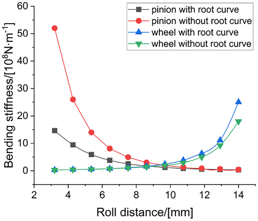
Bending stiffness per unit tooth width.

Figure 12.

Shearing stiffness per unit tooth width.

Figure 13.

Axial compressive stiffness per unit tooth width.

Figure 14.

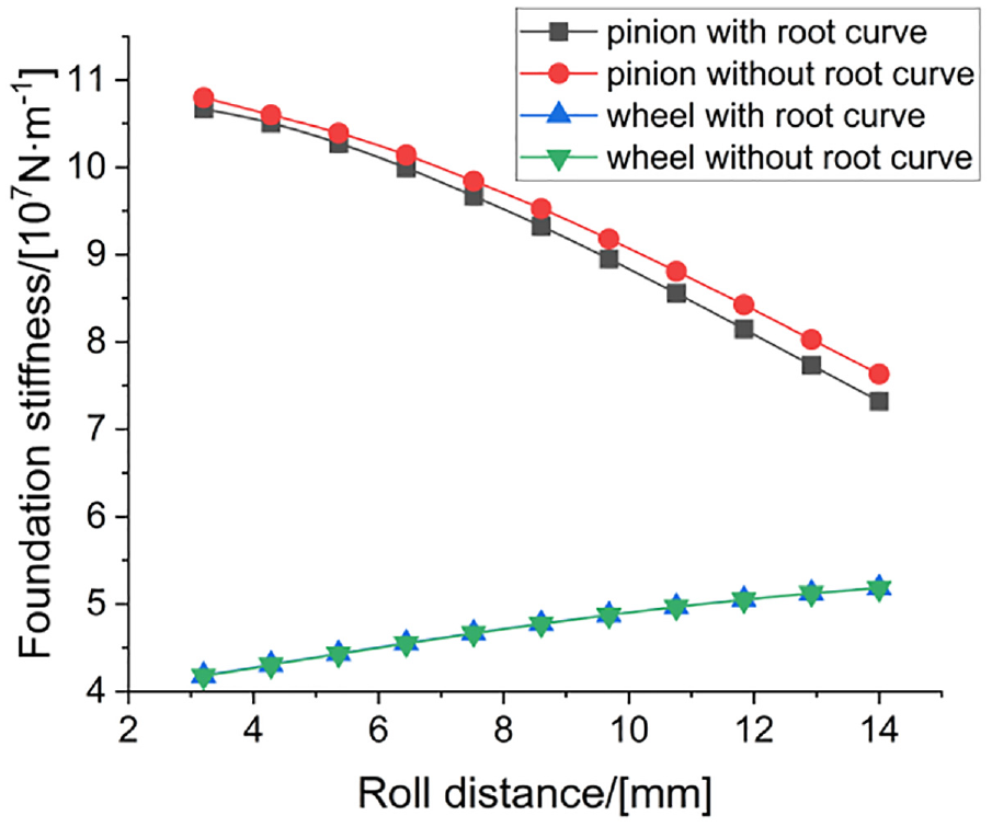
Foundation stiffness per unit tooth.

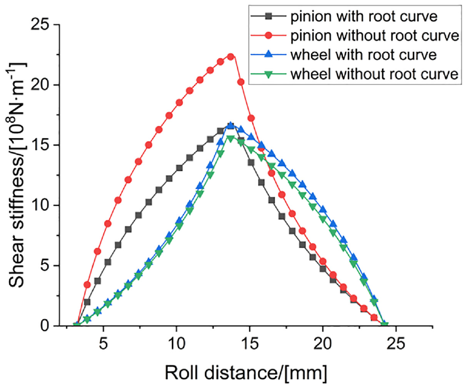
Figures 15 to 18 represent the comparison of single tooth bending stiffness, shear stiffness, axial compression stiffness, and foundation stiffness when considering the tooth root transition curve and not considering the tooth root transition curve. Because the radius of the root circle of the pinion is smaller than the radius of the base circle, the bending stiffness, shear stiffness, axial compression stiffness, and foundation stiffness of the unit tooth width calculated when the root transition curve is considered are smaller than those calculated when the root transition curve is not considered. Therefore, the bending stiffness, shear stiffness, axial compression stiffness, and foundation stiffness of the single tooth calculated when the root transition curve is considered are smaller than those calculated when the root transition curve is not considered. Similarly, because the radius of the root circle of the wheel is slightly larger than the radius of the base circle, the bending stiffness, shear stiffness, axial compression stiffness, and foundation stiffness of the unit tooth width calculated when considering the root transition curve are slightly larger than those calculated when the root transition curve is not considered. Therefore, the bending stiffness, shear stiffness, axial compression stiffness, and foundation stiffness of the single tooth calculated when considering the root transition curve are slightly larger than those calculated when not considering the root transition curve.

Figure 15.

Bending stiffness of single tooth.

Figure 16.

Shearing stiffness of single tooth.

Figure 17.

Axial compressive stiffness of single tooth.

Figure 18.

Foundation stiffness of single tooth.

Figure 19 shows the comparison of the comprehensive meshing stiffness of helical gears considering the tooth root transition curve and not considering the tooth root transition curve. As the gear rotates, the comprehensive meshing stiffness of helical gears changes periodically, so it is called time-varying meshing stiffness (TVMS). The TVMS of helical gears calculated when considering the tooth root transition curve is lower than that calculated when the tooth root transition curve is not considered. Figure 20 shows the helical gear TE when considering the tooth root transition curve and not considering the tooth root transition curve when the torque is 100 Nm. Since the TVMS of the helical gear calculated when considering the tooth root transition curve is lower than that calculated when not considering the tooth root transition curve, the helical gear TE calculated when considering the tooth root transition curve is larger than the helical gear TE calculated when not considering the tooth root transition curve.

Figure 19.

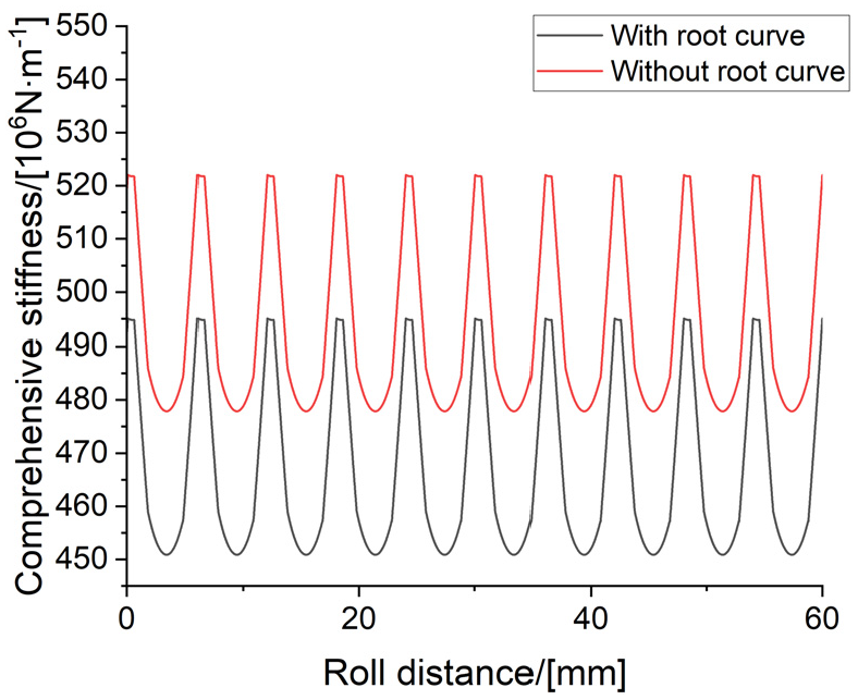
Comprehensive meshing stiffness of helical gear pair.

Figure 20.

Curves of theoretical TE.

Verification of helical gear TE

Experiments were conducted, and the results were compared with theoretical results using the established TE measurement setup, with the aim of further validating the effectiveness of the proposed calculation model for helical gear pair TE.

The experiments were performed at different torque levels from 50 to 300 Nm, while a constant speed of 10 rpm was maintained. The comparison analysis of TE in this study was based on the measured data from multiple meshing cycles. However, only 10 randomly selected meshing cycles were selected for visualization to illustrate the TE curve more clearly. In order to verify the accuracy of the theoretical model proposed in this paper, Figure 21 shows the comparison between the calculated theoretical TE and the experimental TE in 10 meshing cycles considering the root transition curve and not considering the root transition curve. The comparison results show that with the increase of torque, the TE becomes larger. The theoretical TE calculated when considering the root transition curve is greater than the theoretical TE calculated when not considering the root transition curve, and the theoretical TE calculated when considering the root transition curve is closer to the experimental TE. Under certain experimental conditions, the experimental TE of different meshing periods is slightly different, which is mainly caused by the fluctuation of load and speed.

Figure 21.

Curves of theoretical TE and experimental TE: (a) 50 Nm, (b) 100 Nm, (c) 150 Nm, (d) 200 Nm, (e) 250 Nm, and (f) 300 Nm.

To further validate the TE calculation model of the helical gear pair in this paper, the root mean square amplitude of the theoretical TE_RMS and the experimental TE_RMS considering the tooth root transition curve and not considering the tooth root transition curve under different torques is calculated and compared. It can be seen from Table 4 that the TE calculated by considering the tooth root transition curve is closer to the experimental TE than that calculated without considering the tooth root transition curve, and the maximum error is only 8.1%, the precision of the suggested algorithm for TE, which takes into account the root transition curve, is 55% greater than the conventional algorithm for TE that does not consider the root curve.

Table 4.

Comparison table of TE of helical gears.

Torque (Nm)	Experimental TE (μm)	Theoretical TE with root curve (μm)	Theoretical TE without root curve (μm)	Theoretical TE with root curve error (%)	Theoretical TE without root curve error (%)
50	0.18	0.17	0.15	7.30	16.70
100	0.37	0.33	0.30	8.10	10.80
150	0.55	0.52	0.48	5.40	12.70
200	0.74	0.69	0.61	6.20	17.50
250	0.91	0.86	0.77	5.60	15.30
300	1.12	1.03	0.93	7.90	17.00

Parameter analysis and discussion

Gearing design should consider multiple aspects of performance, particularly in terms of automotive transmissions. Factors (e.g. strength, spatial arrangement, cost, standardization, fuel economy, power delivery, and NVH) should be considered. Thus, at the initial stage of gear system design, the center distance and speed ratio are typically not altered. The center distance is affected by parameters (e.g. the number of teeth, module, and helix angle). Isolating the study of individual effects of tooth count, module, and helix angle on mesh stiffness takes on limited significance in practice. The TE of helical gears is determined by a wide variety of factors (e.g. the involute profile, start of active profile (SAP), end of active profile (EAP), transverse contact ratio, and overlap ratio). The design schemes are listed in Table 5. Cases 1–4 represent gear parameters at different pressure angles, Cases 5–8 represent gear parameters for different SAP and EAP, and Cases 9–20 represent gear parameters at different transverse contact ratio and overlap ratio.

Table 5.

Different gear parameters.

Parameter name	Pressure angle (°)	Effective face width (mm)	Start of active profile (mm)	End of active profile (mm)	Base pitch diameter(mm)	Transverse contact ratio (-)	Overlap ratio (-)
Case1	16.0	19.0	4.75	13.47	6.09	1.43	1.71
Case2	18.0	19.0	4.72	13.69	6.01	1.50	1.71
Case3	20.0	19.0	4.68	13.96	5.92	1.57	1.71
Case4	22.0	19.0	6.02	14.09	5.82	1.39	1.71
Case5	18.5	19.0	3.70	14.50	5.99	1.80	1.71
Case6	18.5	19.0	3.50	14.30	5.99	1.80	1.71
Case7	18.5	19.0	3.30	14.10	5.99	1.80	1.71
Case8	18.5	19.0	3.10	13.90	5.99	1.80	1.71
Case9	18.5	16.7	4.50	11.69	5.99	1.20	1.50
Case10	18.5	22.2	4.50	11.69	5.99	1.20	2.00
Case11	18.5	27.8	4.50	11.69	5.99	1.20	2.50
Case12	18.5	33.3	4.50	11.69	5.99	1.20	3.00
Case13	18.5	16.7	3.90	12.89	5.99	1.50	1.50
Case14	18.5	22.2	3.90	12.89	5.99	1.50	2.00
Case15	18.5	27.8	3.90	12.89	5.99	1.50	2.50
Case16	18.5	33.3	3.90	12.89	5.99	1.50	3.00
Case17	18.5	16.7	3.50	14.30	5.99	1.80	1.50
Case18	18.5	22.2	3.50	14.30	5.99	1.80	2.00
Case19	18.5	27.8	3.50	14.30	5.99	1.80	2.50
Case20	18.5	33.3	3.50	14.30	5.99	1.80	3.00

Gear components were fabricated based on a range of design schemes to validate the effect of different gear parameters on TE. TE experiments were performed on a dedicated test rig, and the fabricated components are presented in Figure 22. The experimental conditions covered an input speed of 10 rpm and a torque of 100 Nm. TE were recorded for a wide variety of gear parameters.

Figure 22.

Fabricated components for multiple design schemes.

Effect of pressure angles

The pressure angle is an important factor that affects the TVMS and TE. Many studies have examined the pressure angle in literature. From the research results of Doğan et al.,³⁵ it can be seen that the pressure angle increases from 18° to 30°, and the meshing stiffness increases by $3 \times 10^{5} N / mm$ . From the research results of Zhou et al.,³⁶ it can be seen that the pressure angle increases from 17.5° to 22.5°, and the meshing stiffness increases by $1 \times 10^{5} N / mm$ . Figure 23 illustrates the mesh stiffness of the gear pairs in Case 1 to Case 4 at different pressure angles. The pressure angle is capable of determining the shape of the involute curve. With the rise of the pressure angle, the curvature radius of the involute curve was increased, such that in a wider tooth profile and improved face stiffness of the gears were generated. Moreover, with the increase in the pressure angle, the length of the contact line decreases, while the base pitch of the gear pair decreases as well, resulting in a change in the transverse contact ratio. Therefore, when the pressure angle increases from 16° to 22°, the bending stiffness of a single tooth increases, while the transverse contact ratio initially increases and then decreases. Given the combined effect of face stiffness and transverse contact ratio, the average stiffness initially increases and then decreases as the pressure angle increases from 16° to 22°. The variation amounts to $0.8 \times 10^{5} N / mm$ . The variation law of meshing stiffness with pressure angle studied in this paper differs from Doğan et al.³⁵ and Zhou et al.³⁶ mainly due to the small gear modulus examined in this study. As a result, the changes in meshing stiffness with pressure angle are not significant. The calculation method in this paper takes into account the tooth root transition curve. Compared to the traditional calculation method, the meshing stiffness calculated in this paper is smaller and closer to the actual value. Figure 24 displays a comparison between the theoretical and experimental effective values of the TE for different pressure angles in Case 1 to Case 4. As shown in the figure, the effective value of TE initially decreases and then increases, with the pressure angle ranging from 16° to 22°. Notably, the experimental results were consistent with the expected trends observed in the theoretical analysis.

Figure 23.

Meshing stiffness at different pressure angles.

Figure 24.

Theoretical TE and experimental TE at different pressure angles.

Effect of meshing positions

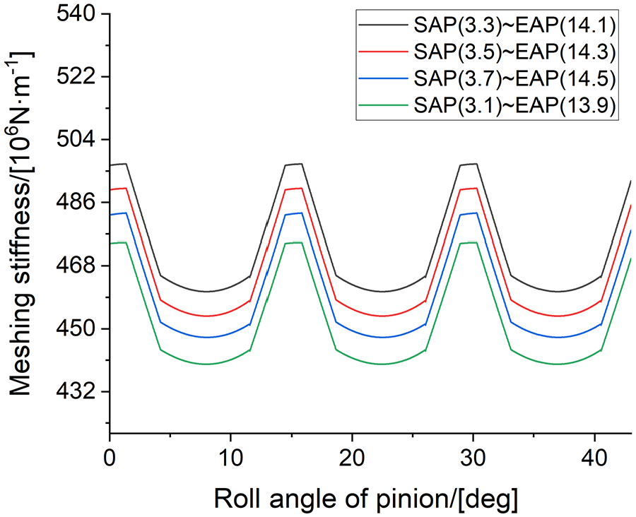
To study the effect of meshing line positions on mesh stiffness, the addendum coefficient and dedendum coefficient were regulated to change the positions of SAP and EAP while keeping the difference between EAP and SAP constant. On that basis, the consistent transverse contact ratio can be ensured. Figure 25 presents the variations in the mesh stiffness for Case 5 to Case 8, with different meshing positions, that is, SAP (3.7 mm)–EAP (14.5 mm), SAP (3.5 mm)–EAP (14.3 mm), SAP (3.3 mm)–EAP (14.1 mm), as well as SAP (3.1 mm)–EAP (13.9 mm). The nodal extension of the gear pair was 8.7 mm. As indicated by the result, when the meshing position is closer to the nodal point, specifically at SAP (3.3 mm) –EAP (14.1 mm), the mesh stiffness was enhanced. Figure 26 illustrates the comparison between the theoretical and experimental effective values of the TE for a range of meshing positions in Case 5 to Case 8. As depicted in the graph, the TE was minimized under the meshing position ranging from SAP (3.3 mm) to EAP (14.1 mm). However, since the TE did not significantly vary with different meshing positions, a slight deviation was identified between the experimental and theoretical results regarding the trend.

Figure 25.

Meshing stiffness at different meshing positions.

Figure 26.

Theoretical TE and experimental TE at different meshing positions.

Effect of overlap ratio

The length of the meshing line, and further the transverse contact ratio, can vary by regulating the addendum coefficient and dedendum coefficient, with the aim of investigating the effect of the overlap ratio on mesh stiffness. The overlap ratio is regulated by changing the tooth width. In this study, the effect of the involute shape on mesh stiffness is excluded, and the focus is only placed on the effect of the overlap ratio.

Figure 27 illustrates the average stiffness for different combinations of transverse contact ratio and overlap ratio (Case 9 to Case 20). With the increase of the transverse contact ratio from 1.2 to 1.8, the average stiffness was increased. Likewise, when the overlap ratio was increased from 1.5 to 3, there was an upward trend in the average stiffness. For a transverse contact ratio of 1.8 and an overlap ratio of 3, the average stiffness reached 8.66 × 10⁸ N/m. Hence, increasing the overlap ratio can contribute to an enhancement of the average stiffness. Figure 28 compares the theoretical and experimental effective values of the TE for various combinations of transverse contact ratio and overlap ratio (Case 9 to Case 20). As the overlap ratio was increased from 1.5 to 3, there was an overall reduction in the TE. However, when the overlap ratio approached 1.5 or 2.5, the peak-to-peak value of the TE started to rise. Moreover, with the increase of the transverse contact ratio from 1.2 to a value close to 1.5, the peak-to-peak value of the TE tended to be increased. When the overlap ratio was 1.5 and the transverse contact ratio was 1.5, the maximum recorded effective value of the TE reached 2.69 μm. Notably, the experimental results were consistent with the theoretical results, thus demonstrating a high level of agreement.

Figure 27.

Average stiffness of combinations with different contact ratios.

Figure 28.

TE_RMS at different contact ratios.

Conclusion

In this study, a novel algorithm is presented for correcting TE in helical gears in accordance with the potential energy method. The algorithm considers the root transition curve formed by the trajectory of the tool in the rolling motion. Moreover, an experimental setup was established to validate the theoretical findings. As indicated by the result of the comparative analysis of theory and experiments, the TE considering the tooth root transition curve is closer to the experimental TE than the TE without considering the tooth root transition curve. The error between the TE considering the tooth root transition curve and the experimental TE is significantly higher than that between the TE without considering the tooth root transition curve and the experimental TE. The maximum error between the TE considering the tooth root transition curve and the experimental TE is only 8.1%, the precision of the suggested algorithm for TE, which takes into account the root curve, is 55% greater than the conventional algorithm for TE that does not consider the root curve. The effect of multi-parameters (e.g. pressure angle, start of active profile (SAP), end of active profile (EAP), transverse contact ratio, and overlap ratio) on TE was investigated by a comparative analysis between theory and experiments. The following conclusions can be drawn:

(1) With the rise of the pressure angle, the curvature radius of the involute curve is increased, such that the face stiffness of the gear is enhanced. Moreover, at a higher pressure angle, the transverse contact ratio is first increased and then decreased. Accordingly, under the combined effect of face stiffness and transverse contact ratio, the average mesh stiffness tends to be first increased and then decreased. The effective value of the TE, which is affected by the time-varying mesh stiffness, is first decreased and then increased. The experimental results are consistent with the theoretical results.

(2) When the meshing position is closer to the nodal point, the mesh stiffness is slightly enhanced, resulting in a minor reduction in the TE. However, since the variation in the TE is insignificant across different meshing positions, some discrepancy exists between the experimental and theoretical results.

(3) Increasing the overlap ratio leads to an increase in average stiffness and an overall decrease in the TE. However, the TE reaches its maximum value when the overlap ratio approaches the odd multiples of 0.5. The experimental results are well consistent with the theoretical results, thus demonstrating a high degree of agreement. Thus, in the gear design, it is crucial to appropriately match gear parameters. On the one hand, a larger overlap ratio should be ensured to engage more teeth in meshing and enhance average stiffness. On the other hand, the overlap ratio should be approach an integer to minimize TE and enhance the NVH performance of the gear system.

Footnotes

Appendix

Handling Editor: Chenhui Liang

Declaration of conflicting interests

The author(s) declared no potential conflicts of interest with respect to the research, authorship, and/or publication of this article.

Funding

The author(s) received no financial support for the research, authorship, and/or publication of this article.

ORCID iD

Ziqian Liu

References

Marafona

JDM

Marques

PMT

Martins

, et al. Mesh stiffness models for cylindrical gears: a detailed review. Mech Mach Theory 2021; 166: 104472.

Duan

Wei

Zhang

, et al. Transmission error investigation of gearbox using rigid-flexible coupling dynamic model: theoretical analysis and experiments. Mech Mach Theory 2021; 157: 104213.

Rezayat

Catera

Capalbo

, et al. Numerical and experimental analysis of the transmission error in hybrid metal-composite gears. Compos Struct 2022; 298: 116012.

Pandya

Parey

. Experimental investigation of spur gear tooth mesh stiffness in the presence of crack using photoelasticity technique. Eng Fail Anal 2013; 34: 488–500.

Raghuwanshi

Parey

. Experimental measurement of gear mesh stiffness of cracked spur gear by strain gauge technique. Measurement 2016; 86: 266–275.

Raghuwanshi

Parey

. Experimental measurement of mesh stiffness by laser displacement sensor technique. Measurement 2018; 128: 63–70.

Abruzzo

Beghini

Santus

, et al. Dynamic behavior of a power re-circulating gear test rig including periodic variation of mesh stiffness and static transmission error. Mech Mach Theory 2021; 159: 104247.

Hedlund

Lehtovaara

. A parameterized numerical model for the evaluation of gear mesh stiffness variation of a helical gear pair. Proc IMechE, Part C: J Mechanical Engineering Science 2008; 222: 1321–1327.

Cooley

Liu

Dai

, et al. Gear tooth mesh stiffness: a comparison of calculation approaches. Mech Mach Theory 2016; 105: 540–553.

10.

Abruzzo

Beghini

Santus

, et al. A dynamic model combining the average and the local meshing stiffnesses and based on the static transmission error for spur gears with profile modification. Mech Mach Theory 2023; 180: 105139.

11.

Lin

. Analytical method for coupled transmission error of helical gear system with machining errors, assembly errors and tooth modifications. Mech Syst Signal Process 2017; 91: 167–182.

12.

Velex

Sainsot

, et al. Analytical investigations on the mesh stiffness function of solid spur and helical gears. J Mech Des 2015; 137: 063301.

13.

Zheng

Luo

, et al. Analytical approach to mesh stiffness modeling of high-speed spur gears. Int J Mech Sci 2022; 224: 107318.

14.

Sun

Tang

Chen

, et al. Mesh stiffness and dynamic response analysis of modified gear system with thin web and weight reduction holes. J Sound Vib 2023; 546: 117437.

15.

Wan

Cao

, et al. An improved time-varying mesh stiffness algorithm and dynamic modeling of gear-rotor system with tooth root crack. Eng Fail Anal 2014; 42: 157–177.

16.

Tang

Zou

Yang

, et al. Novel mathematical modelling methods of comprehensive mesh stiffness for spur and helical gears. Appl Math Model 2018; 64: 524–540.

17.

Xie

Hua

Lan

, et al. Improved analytical models for mesh stiffness and load sharing ratio of spur gears considering structure coupling effect. Mech Syst Signal Process 2018; 111: 331–347.

18.

Wei

Zhang

Wang

, et al. A study of nonlinear excitation modeling of helical gears with modification: theoretical analysis and experiments. Mech Mach Theory 2018; 128: 314–335.

19.

Wan

Cao

, et al. Mesh stiffness calculation using an accumulated integral potential energy method and dynamic analysis of helical gears. Mech Mach Theory 2015; 92: 447–463.

20.

Chung

W-J

Park

J-H

Yoo

H-G

, et al. Improved analytical model for calculating mesh stiffness and transmission error of helical gears considering trochoidal root profile. Mech Mach Theory 2021; 163: 104386.

21.

Sun

Chen

, et al. Analytical models for thermal deformation and mesh stiffness of spur gears under steady temperature field. Eng Fail Anal 2022; 133: 105972.

22.

Yang

Wang

Shao

, et al. A double-layer iterative analytical model for mesh stiffness and load distribution of early-stage cracked gear based on the slicing method. Mech Syst Signal Process 2023; 198: 110456.

23.

Yang

Tang

, et al. Research on the time-varying mesh stiffness method and dynamic analysis of cracked spur gear system considering the crack position. J Sound Vib 2023; 548: 117505.

24.

Zheng

Luo

, et al. Study on the mesh stiffness and nonlinear dynamics accounting for centrifugal effect of high-speed spur gears. Mech Mach Theory 2022; 170: 104686.

25.

Chen

Lei

, et al. A study of effects of tooth surface wear on time-varying mesh stiffness of external spur gear considering wear evolution process. Mech Mach Theory 2021; 155: 104055.

26.

Dai

Long

Chen

, et al. An improved analytical model for gear mesh stiffness calculation. Mech Mach Theory 2021; 159: 104262.

27.

Wang

Zhu

. An improved mesh stiffness model of helical gear pair considering axial mesh force and friction force influenced by surface roughness under EHL condition. Appl Math Model 2022; 102: 453–471.

28.

Yang

Tang

, et al. Dynamic analysis for a spur geared rotor system with tooth tip chipping based on an improved time-varying mesh stiffness model. Mech Mach Theory 2021; 165: 104435.

29.

Chen

Zhou

Zhai

, et al. Improved analytical calculation model of spur gear mesh excitations with tooth profile deviations. Mech Mach Theory 2020; 149: 103838.

30.

Han

. Influences of tooth spalling or local breakage on time-varying mesh stiffness of helical gears. Eng Fail Anal 2017; 79: 75–88.

31.

Zhu

Liu

, et al. Mesh stiffness and nonlinear dynamic response of a spur gear pair considering tribo-dynamic effect. Mech Mach Theory 2020; 153: 103989.

32.

Yang

Cao

, et al. Nonlinear dynamic response of a spur gear pair based on the modeling of periodic mesh stiffness and static transmission error. Appl Math Model 2019; 72: 444–469.

33.

Cui

Zhai

Zhang

. Research on the meshing stiffness and vibration response of cracked gears based on the universal equation of gear profile. Mech Mach Theory 2015; 94: 80–95.

34.

Choi

Ahn

Park

, et al. Influence of gear tooth addendum and dedendum on the helical gear optimization considering mass, efficiency, and transmission error. Mech Mach Theory 2021; 166: 104476.

35.

Doğan

Karpat

Kopmaz

, et al. Influences of gear design parameters on dynamic tooth loads and time-varying mesh stiffness of involute spur gears. Sādhanā 2020; 45: 1–15.

36.

Zhou

Xing

. A mesh stiffness model with the asperity contact for spur gear in mixed elastohydrodynamic lubrication. J Braz Soc Mech Sci Eng 2022; 44: 466.

Improved analytical model for calculating mesh stiffness and transmission error of helical gears considering root curve: Theoretical analysis and experiments

Abstract

Keywords

Introduction

Analytical model

Consideration of tooth root curve in helical gear equations

Mesh stiffness of helical gears

Transmission error of helical gear pairs

Transmission error verification

Transmission error experiment

Theoretical calculation of helical gear TE

Verification of helical gear TE

Parameter analysis and discussion

Effect of pressure angles

Effect of meshing positions

Effect of overlap ratio

Conclusion

Footnotes

Appendix

Declaration of conflicting interests

Funding

ORCID iD

References