Sage Journals: Discover world-class research

Abstract

To enhance the efficiency and load-carrying capacity of the jumping robot’s transmission system, the transmission characteristics of the planthopper hip gear were analyzed. The analysis revealed that the gear pair exhibited low transmission errors, high transmission efficiency, and significant torque capacity, making it suitable for high-speed, high-precision, and high-power density transmissions. A bionic design study of the jumping robot’s gear was conducted, drawing inspiration from the planthopper hip gear’s tooth shape and profile. A logarithmic spiral was assumed as the tooth profile based on its consistent pitch angle and curvature gradient characteristics. Parameters of the tooth profile of the bionic gear were calculated, and equations for the tooth surface were derived. A three-dimensional model of the bionic gear was constructed, and both its transmission efficiency and error were calculated. Using the finite element method, theoretical formulas for contact stress and bending stress in the bionic gear were deduced. The distribution characteristics of both bending and contact stress were analyzed, demonstrating that the bionic gear used in high-performance jumping robots possesses low transmission error, high transmission efficiency, and excellent contact strength, providing a theoretical foundation for enhancing their jumping capabilities.

Keywords

Bionic gear logarithmic spiral tooth profile meshing principle transmission performance strength analysis

Introduction

Jumping robots exhibit the remarkable capability to traverse obstacles tenfold or even several tens of times their size. This ability holds immense value and offers extensive application possibilities in interstellar exploration, terrain investigation, ore prospecting, and enemy detection. Most jumping robots store energy by propelling energy storage elements through a multi-stage variable-speed drive mechanism to enable their jumping motion.^1,2 The pressure angle in the gear drive system of the jumping robot varies significantly, leading to substantial dynamic loads on the system.^3,4 Gear pairs serve as fundamental components within the jumping robot transmission system and have a profound impact on transmission efficiency and load-carrying capacity, which, in turn, influence the jumping capacity of the robot. Therefore, the development of high-performance gears suitable for jumping robot transmission systems holds significant importance and offers extensive technical applications for enhancing the jumping abilities of these robots.

Jumping insects, after thousands of years of evolution, have excellent jumping abilities in natural environments. Based on biomimetic principles, the physiological structure of jumping insects is simulated to design mechanical structures with similar functions, which is an important way to improve the jumping performance of jumping robots. Zoologists Malcolm Burrows and Gregory Sutton, affiliated with the University of Cambridge, were the first to identify a gear-shaped biological structure in the planthopper,⁵ situated in their hips (as depicted in Figure 1). This gear rapidly rotates and facilitates the synchronized movement of the planthopper’s left and right legs during jumping. The planthopper, having evolved over an extensive period in its natural habitat, demonstrates a remarkable adaptation to its environment. The hip gear of the planthopper, a vital component in its jumping mechanism, exhibits characteristics of high synchronization accuracy and relative output torque.⁵ To meet the demands for high transmission efficiency and load-carrying capacity in jumping robots, we have designed a new type of gear pair. This design draws inspiration from the structural features of the planthopper’s hip gear pair, with the goal of achieving higher transmission efficiency, synchronization accuracy, and load capacity. A new type of gear is designed to meet the requirements of high-performance jumping robots for transmission efficiency and load capacity.

Figure 1.

Planthopper and its hip gear pair.⁵

The tooth profile of the planthopper hip gear occurs naturally, while the logarithmic spiral is a naturally occurring curve known for its simplicity, structural stability, and uniform pitch angle. Incorporating the logarithmic spiral into the bionic design of the planthopper hip joint gears offers a fresh perspective. The logarithmic spiral’s consistent pitch angle addresses issues related to high dynamic loads and unstable transmission, which stem from wide fluctuations in pressure angles within the gear transmission of jumping robots.⁶ Furthermore, the curvature gradient characteristic of the logarithmic spiral tackle problems such as gear wear, power loss, and fatigue failure arising from variations in the curvature of gear tooth profiles.⁷ In recent years, logarithmic helix has gradually been applied to the tooth profile of bevel gear transmission, and the tooth profile of this type of bevel gear is still involute or circular.^8,9 Yang¹⁰ proposed that an imaginary rack cutter with the tooth shape of the planthopper could be used to generate a pair of gears. Multiple circular arcs were used to fit tooth profiles of the planthopper hip gear.

As a result, this paper introduces the hypothesis that the working tooth profile of the hip gear is a logarithmic spiral. Leveraging the tooth shape and tooth profile attributes of the planthopper hip gear, a novel bionic gear is developed, considering the mathematical properties of the logarithmic spiral. The meshing characteristics and transmission performance of the bionic gear are analyzed to enhance efficiency, thereby contributing to the improved efficiency and load capacity of the jumping robot’s transmission system.

Analysis of transmission characteristics of planthopper hip gear

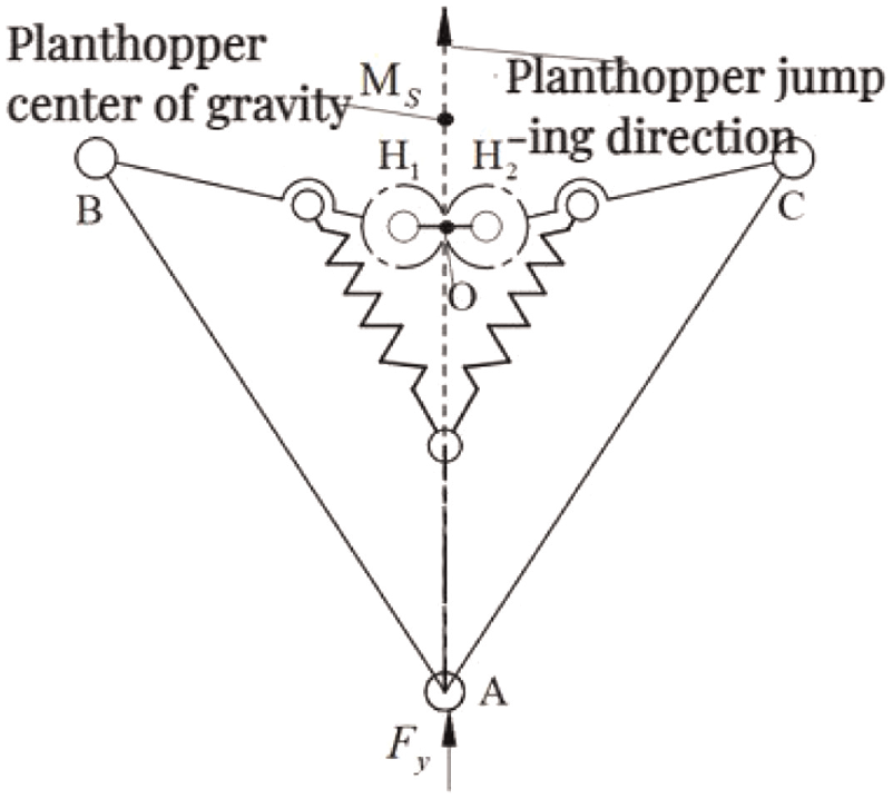
During the planthopper jumping process, the leg and tibia segments with the most significant influence on jumping are considered in the planthopper’s jumping foot, while other limb segments are simplified. The weight of the jumping foot is not factored into the analysis, as it typically constitutes a small proportion of the insect’s total body weight (generally less than 10%).¹¹ As depicted in Figure 2, the planthopper’s jumping structure is simplified to comprise the hip gears H₁ and H₂, with O representing the gear contact point and M_S as the center of gravity for the planthopper’s body. H₁B and H₁C denote the leg segments, while AB and AC represent the tibia segments. The upward jumping force, F_y, is generated at the point of contact between A and the ground.

Figure 2.

Simplified model of planthopper jumping foot.

The planthopper hip gears are always in a meshing state during the jumping process. Each joint angle is shown in Figure 3(a). Referring to the literature,¹¹ the leg-ground angle α during the planthopper jumping is obtained, and a polynomial function is used for fitting. The planthopper hip gear speed is acquired by the derivation of the leg-ground angle α, as depicted in Figure 3(b). The maximum speed of the planthopper hip gear is 12000 r/min, indicating that the gear is used in high-speed transmission.¹²

Figure 3.

Planthopper jumping foot model and its speed: (a) Jumping foot model and (b) The angular speed of the planthopper hip gear.

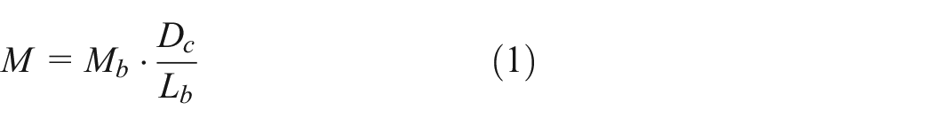
According to the literature,⁵ the maximum output torque T_out of the planthopper hip gear drive is 0.7 mN.mm. The average weight M_b of the planthopper is 6.6 mg. Its average body length L_b is 4.1 mm, and the diameter D_c of the planthopper hip gear is about 0.4 mm. To calculate the maximum output power P of the planthopper hip gear, the weight M of the planthopper hip gear pairs can be calculated in proportion to their length, as depicted in equation (1).

M = M_{b} \cdot \frac{D_{c}}{L_{b}}

(1)

The power density of the planthopper hip gear drive is 1.3743 kW/kg, which is used in the high-power density drive.¹³

The transmission error $θ_{er}$ of the gear refers to the relative difference between the actual angle $θ_{out}$ of the output shaft and the theoretical angle $(θ_{in} / i)$ when the input shaft rotates at any angle,¹⁴ as depicted in equation (9).

θ_{er} = θ_{out} - \frac{θ_{in}}{i}

(2)

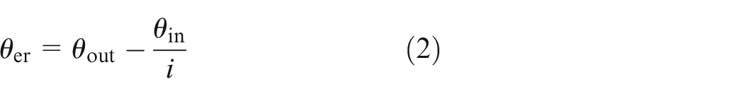
Where i is the transmission ratio.

Referring to the literature,⁵ it is known that the whole jumping time of the planthopper is 78.4 ms, and the time error is 21 μs. The jumping acceleration time is 1.8 ms. t_er is the error of the jumping acceleration time, as equation (3).

t_{er} = \frac{t_{in}}{t_{all}} \cdot t_{aer}

(3)

Where t_in is the jumping acceleration time; $t_{all}$ is the whole jumping time; t_aer is the time error.

The driving gear rotates 90° during acceleration (θ_in). And the average angular velocity ω_in of the driving gear is obtained as equation (4).

ω_{in} = \frac{θ_{in}}{t_{in}}

(4)

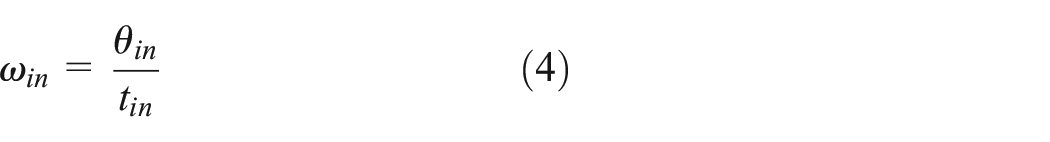
The planthopper hip gear pair ensures precise synchronization, i = 1. The average angular velocity ω_in of the driving gear is equal to the average angular velocity ω_out of the driven gear, that is, ω_in = ω_out. The transmission error θ_er can be obtained as equation (5).

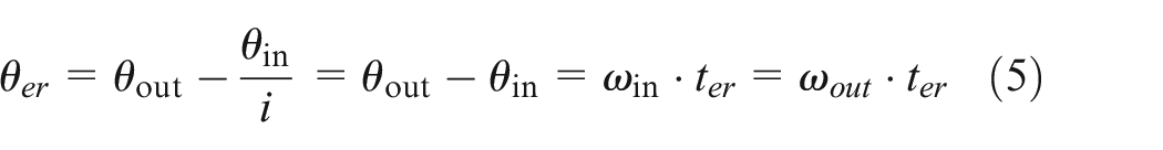
θ_{er} = θ_{out} - \frac{θ_{in}}{i} = θ_{out} - θ_{in} = ω_{in} \cdot t_{er} = ω_{out} \cdot t_{er}

(5)

The transmission error time t_er of the planthopper hip gear is 0.5 μs, and the average angular velocity ω_in is 8333.3 r/min. The transmission error of the planthopper hip gear is 36” at an angle of 360° angle, which is a high-precision transmission.^15,16

Assume that the input power of the planthopper hip gear is P_in and the output power during the jump acceleration is P_out. The angular displacement of the driving gear (H₁) is S_in, and that of the driven gear (H₂) is S_out. Because of the symmetry of the planthopper’s jumping foot, it is known that F₁ = F₂. Since the radii of the planthopper hip gears are equal, the arc length is S_in = S_out. The transmission efficiency of the hip gear is given by equation (6).

η = \frac{P_{out}}{P_{in}} = \frac{F_{2} \cdot \frac{S_{out}}{t_{in} + t_{er}}}{F_{1} \cdot \frac{S_{in}}{t_{in}}} = \frac{t_{in}}{t_{in} + t_{er}}

(6)

The transmission efficiency of the planthopper hip gear transmission is 99.97% as depicted in equation (6), which is a high-efficiency transmission device.¹⁷

Bionic design of planthopper hip gear

Analysis of tooth profile characteristics of planthopper hip gear

Mathematical properties of logarithmic spirals

Logarithmic spirals are some of the most amazing curves in nature, ranging from tornado and star orbits to nautilus and spiral fungal structures, as depicted in Figure 4. Conch shells grow naturally with the growth of organisms. And they behave with great strength and toughness. The spider’s web, winding around the center, achieves infinite extension outwards in a logarithmic spiral shape. These phenomena show that logarithmic spirals are the products of natural selection.

Figure 4.

Natural logarithmic spiral.

The logarithmic spiral has the following properties: (1) the pitch angles of each point on the same logarithmic spiral are equal everywhere; (2) a logarithmic spiral is an equidistant curve; (3) its evolute and vertical traces are still logarithmic spirals; (4) the radius of gradient curvature is an increasing function of the polar angle.

Extraction and fitting of planthopper hip gear tooth

Considering the actual tooth profile of the planthopper hip gear, the edge detection method¹⁷ is used to identify and extract its working tooth profile. Inspired by nature, the working tooth profile of planthopper hip gear is assumed to be a logarithmic helical.

(1) Binarization processing

The original images of the gear teeth of the planthopper hip gear are acquired as depicted in Figure 5.

Figure 5.

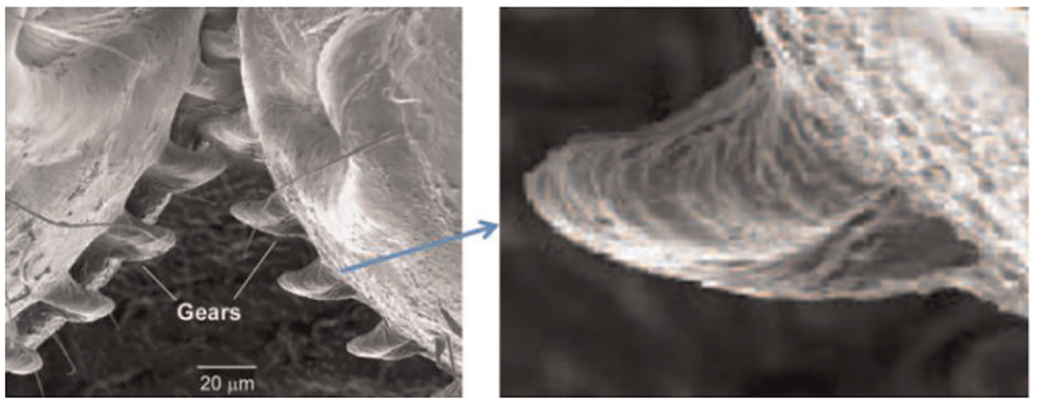
Planthopper hip gear.

The adaptive thresholding binarization method¹⁸ is used to binarize Figure 5. If the grey value of the pixel is greater than the adaptive threshold 128, the pixel is displayed as white; if it is less than the adaptive threshold 128, the pixel is displayed as black. The custom denoising method¹⁸ is used to further suppress the noise in the background of the binary image. As depicted in Figure 6(a)–(d), the binarized images of the planthopper hip gear with different denoising thresholds are obtained. From Figure 6(c), it can be seen that the edge contour of the planthopper hip gear is complete, with no noise points near the contour, which is selected for further tooth profile extraction.

Figure 6.

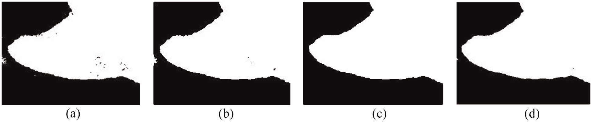
Noise plots for different thresholds after binarization of the planthopper hip gear: (a) Denoising thresholds: 5, (b) Denoising thresholds: 10, (c) Denoising thresholds: 15 and (d) Denoising thresholds: 20.

(2) Extraction and segmentation of the planthopper hip gear profile

The extracted marginal tooth profile of Figure 6(c) is depicted in Figure 7(a), which is not smooth. The marginal tooth profile is then smoothed¹⁹ to obtain the smooth planthopper hip tooth profile as depicted in Figure 7(b).

Figure 7.

Smoothing of the tooth profile: (a) Before smoothing and (b) After smoothing.

Figure 8 shows the conceptual diagram of the tooth profile comparison between the planthopper hip gear and the involute gear.⁵ According to the real size of the planthopper hip gear, the tooth height of the planthopper hip gear is 30 μm. The dedendum of the planthopper hip gear is 16.67 mm and the addendum is 13.33 mm, referring to the distribution ratio of the dedendum and addendum of the standard involute gear. The tooth profile of the planthopper hip gear is segmented based on the involute gear meshing principle.²⁰ Curves AB and EF are the root transition tooth profile, the curves BC and DE are the working tooth profile and curve CD is the top transition curve. The nodes of the planthopper gear are the points of intersection k1 and k2 of the nodal line with the working tooth profiles BC and DE.

Figure 8.

Comparison of planthopper hip gear with conventional involute gear.⁵

According to the above method of segmentation and node determination, the real extracted tooth profile of the planthopper hip gear is segmented as depicted in Figure 9(a). To study the characteristics of the working tooth profile BC and DE of the planthopper hip gear, the working tooth profile BC and DE are extracted separately as depicted in Figure 9(b), and the working tooth profile BC and DE are referred to as the convex tooth profile and the concave tooth profile, respectively.

Figure 9.

Extraction of the working tooth profile of the planthopper hip gear: (a) Segmented tooth profile and (b) The working tooth profile.

(3) Fitting the logarithmic spiral function to the working tooth profile of the planthopper hip gear.

The parametric equation of the logarithmic spiral is shown as equation (7)²¹:

{\begin{matrix} x (θ) = r_{0} e^{t θ} \cos θ \\ y (θ) = r_{0} e^{t θ} \sin θ \end{matrix}

(7)

where r₀ is the starting circle radius; t is a constant; and θ is the polar angle.

According to the principle of least squares,²² it is transformed into a minimum value of the sum of the error squares, which is solved step by step using an iterative method. The coordinate transformation of the parametric equation of the logarithmic spiral in the Oxyz plane is given by equation (8).

{\begin{matrix} x (θ) = r_{0} e^{t θ} \cos θ + a_{d} \\ y (θ) = - r_{0} e^{t θ} \sin θ + b_{d} \end{matrix}

(8)

where a_d is the variation in the horizontal coordinate of the logarithmic spiral and b_d is the variation in the vertical coordinate of the logarithmic spiral.

The extracted convex tooth profile BC is translated so that the end point B of the convex tooth profile coincides with the coordinate origin. Similarly, the extracted concave tooth profile DE is translated so that the end point D of the tooth profile coincides with the coordinate origin. The processed convex tooth profile BC and the concave tooth profile DE are fitted separately as depicted in Figure 10(a) and (b). The fitted logarithmic spiral parameters are depicted in Table 1, and the errors are depicted in Table 2.

Figure 10.

The fitted logarithmic spiral of the concave and convex tooth profiles: (a) The fitted convex tooth profile and (b) The fitted concave tooth profile.

Table 1.

Parameters of the logarithmic spiral fitting equation.

Fitted tooth profile	Starting circle, radius r₀ (μm)	Constants, t	Range of polar angle θ (°)	Amount of change in horizontal coordinate $a_{d}$ (μm)	Amount of change in vertical coordinate $b_{d}$ (μm)
Convex profile BC	42.1	−0.0025	(0, 25.67)	0	42.1
Concave profile DE	43.7	−0.0060	(0, 16.48)	0	43.7

Table 2.

Fitting error of the working tooth profile and logarithmic spiral.

Fitted tooth profile	Determination factor R-square	Relative error of the maximum fitting error point (%)	Relative error of nodes (%)
Convex profile BC	0.9916	0.25	0.06
Concave profile DE	0.9938	0.10	0.01

The determination factor of the fitted convex and concave tooth profiles are both greater than 0.99, and the maximum relative error is within 0.25%, indicating that the logarithmic spiral fits the convex and concave tooth profiles with high accuracy. It also verifies the assumption that the working tooth profile of the planthopper hip gear is a logarithmic spiral.

Research on the bionic gear tooth profile design

Construction of logarithmic spiral gear tooth shape of bionic gear

The characteristics of the planthopper hip gear are: (i) the tooth profile is a concave-convex asymmetric tooth profile; (ii) the teeth of the meshing gears are concave-convex meshing, which achieves bidirectional transmission. According to the principle of gear meshing,²³ the conditions for meshing concave-convex meshing gear pairs are: (i) the meshing tooth profile must be a smooth curve; (ii) two tooth profiles mesh at one point, and the common normal of the contact point must pass through the node; (iii) the gear is a helical gear.

The bionic tooth profile of the planthopper hip gear is adjusted to comply with the meshing principle. The planthopper hip gear profile is depicted is Figure 11(a) by referring to the pitch position of the involute gear profile. The center point of the convex tooth profile is O₁, the pressure angle is θ₀, the center point of the concave tooth profile is O₃, the pressure angle is θ₃, and the tooth top height and tooth root height of the gear are $h_{a}$ , $h_{f}$ , respectively. According to the principle of gear meshing,²⁰ the pressure angles on both sides of the tooth profile are guaranteed to be equal in size, that is, θ₀ = θ₃, as depicted in Figure 11(b). The contact points k1 and k2 on both sides of the tooth profile are on the nodal line to satisfy the requirements of the common normal through the node. And the teeth are helical. To ensure that the tooth profile is simple and easy to machine, the adapted bionic tooth profile is further simplified, as depicted in Figure 11(c). The upper transition curve CD is a part of the upper circle of the tooth. The working tooth profiles BC and DE are logarithmic spirals, and smooth circular arcs are adopted for the root transition curves AB and EF,²⁴ as depicted in Figure 11(c). According to the pure rolling contact characteristics of the planthopper hip gear, the contact points on both sides of the tooth profile are limited to the gear nodal line in the design of the bionic gear to achieve theoretical pure rolling.

Figure 11.

Schematic diagram of the adjusted bionic tooth profile: (a) The planthopper hip gear profile, (b) The pressure angle on both sides and (c) The simplified tooth profile.

Design of logarithmic spiral tooth profile parameters for bionic gears

S_s ₁ (P₁−x_s₁y_s₁) (depicted in Figure 12) is the coordinate system established with the center point of the gear pitch thickness P₁ as the origin, the center line of the pitch tooth thickness as the y_s₁ axis, and the pitch line as the x_s₁ axis. S_s₂ (P₂−x_s₂y_s₂) is the coordinate system established where the center point of the gear tooth thickness is the origin P₂, the tooth thickness center line is the y_s₂ axis and the pitch line is the x_s₂ axis. The angle range of the convex tooth profile of the logarithmic helix is (θ₁, θ₂). Its pressure angle is θ₀. The center point is O₁, which has the coordinates (w₁, −f₁) in the coordinate system S_s₁ (P₁−x_s₁y_s₁). The angular range of the concave tooth profile of the logarithmic spiral on the other side of the same gear tooth is (θ₄, θ₅). Its pressure angle is θ₃. The center point is O₃ with coordinates (w1, −f1) in the coordinate system S_s₂ (P₂−x_s₂y_s₂) with coordinates (w₂, f₂). The pressure angles of the logarithmic spiral convex and concave tooth profiles are equal in size, that is, θ₀ = θ₃. The vertical distance from the root transition point to the nodal line of the logarithmic spiral convex and concave tooth profiles are h_g₁ and h_g₂. Its tooth top height and tooth root height are h_a and h_f. The tooth thickness of the gear is s. The side clearance is j, and the tooth slot width is s + j. The parameter formulas of the bionic gear tooth profile are derived as depicted in Table 3.

Figure 12.

Bionic gear tooth profile parameters.

Table 3.

Tooth profile and transition arc calculation formulae.

Curve section name	Parameter name	Parameter calculation formula
Convex profile working section	Convex tooth profile process angle θ₁	—
	Convex tooth profile termination angle θ₂	$θ_{2} = \arcsin [(h_{a} + f_{1}) / (r_{1} e^{t \times θ_{2}})]$
	Lateral offset of convex tooth profile w₁	$w_{1} = r_{1} e^{t \times θ_{0}} \cos θ_{0} - s / 2$
	Longitudinal offset of convex tooth profile f₁	$f_{1} = r_{1} e^{t \times θ_{0}} \sin θ_{0}$
	Radius of convex tooth profile transition arc r_g1	$r_{g 1} = (r_{1} e^{t \times θ_{1}} \sin θ_{1} - f_{1} + h_{f}) / (1 - \sin θ_{1})$
Concave profile working section	Concave tooth profile process angle θ₄	$θ_{4} = \arcsin [(r_{2} e^{t \times θ_{3}} \sin θ_{3} - h_{a}) / (r_{2} e^{t \times θ_{4}})]$
	Concave tooth profile termination angle θ₅	—
	Lateral offset of concave tooth profile w₂	$w_{2} = r_{2} e^{t \times θ_{3}} \cos θ_{3} - (s + j) / 2$
	Longitudinal offset of concave tooth profile f₂	$f_{2} = r_{2} e^{t \times θ_{3}} \sin θ_{3}$
	Radius of concave tooth profile transition arc r_g2	$r_{g 2} = (h_{f} - r_{2} e^{t \times θ_{5}} \sin θ_{5} + f_{2}) / [1 - \cos (π / 2 - θ_{5})]$

3D modeling of the bionic gear

The angle between the center line of the adjacent teeth of the planthopper gear is about 8.5°. If the teeth are distributed over the whole circle, the number of teeth is about 42. Therefore, the number of teeth in the bionic gear pair is 42. The size of the planthopper gear is enlarged by 100 times. The height of the bionic gear tooth is 3 mm. Referring to the pure rolling single arc gear,²⁴ the dedendum and addendum are 1.8 and 1.2 mm respectively, as depicted in Table 4.

Table 4.

Basic parameters of the bionic gear.

Setting parameters	Numerical value	Calculation parameters	Numerical value
Number of teeth $z_{1} / z_{2}$	42/42	Thick teeth $s$ (mm)	4.62
Normal modulus $m_{n}$ (mm)	3	Wide cogging $e$ (mm)	4.8
Tooth top height factor $h_{a}^{*}$	0.4	Side Gap $j$ (mm)	0.18
Top gap coefficient $c^{*}$	0.2	Diameter of indexing circle $d$ (mm)	133.0008
Tooth width $b$ (mm)	44	Tooth top circle diameter $d_{a}$ (mm)	135.4008
Spiral Angle $β$ (°)	18.6727	Diameter of tooth root circle d_f (mm)	129.4008
Pressure angle $θ_{0} / θ_{3}$ (°)	24	Tooth top height $h_{a}$ (mm)	1.2
Center Distance $a$ (mm)	133.0008	Tooth root height h_f (mm)	1.8
Lateral clearance coefficient $j^{*}$	0.06	Longitudinal overlap	1.4947

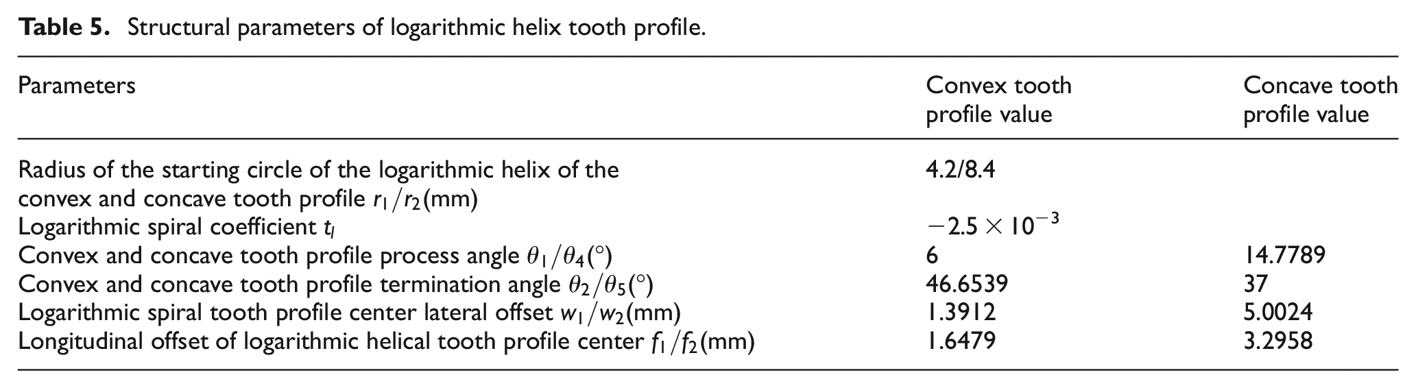
According to the fitting results in Table 1, the starting circle radius of the convex tooth profile is r₁ = 4.2 mm, and the logarithmic helix coefficient is t_l =−2.5 × 10⁻³ after the gear is amplified 100 times. To ensure that the gear does not interfere, the starting circle radius of the concave tooth profile is r₂ = 8.4 mm, θ₁ = 6° and θ₅ = 37°. Structural parameters of logarithmic helix tooth profile are depicted in Table 5.

Table 5.

Structural parameters of logarithmic helix tooth profile.

Parameters	Convex tooth profile value	Concave tooth profile value
Radius of the starting circle of the logarithmic helix of the convex and concave tooth profile $r_{1} / r_{2}$ (mm)	4.2/8.4
Logarithmic spiral coefficient $t_{l}$	−2.5 × 10⁻³
Convex and concave tooth profile process angle $θ_{1} / θ_{4}$ (°)	6	14.7789
Convex and concave tooth profile termination angle $θ_{2} / θ_{5}$ (°)	46.6539	37
Logarithmic spiral tooth profile center lateral offset $w_{1} / w_{2}$ (mm)	1.3912	5.0024
Longitudinal offset of logarithmic helical tooth profile center $f_{1} / f_{2}$ (mm)	1.6479	3.2958

The normal meshing tooth profile of the bionic gear is drawn and projected onto the end face to obtain the end meshing tooth profile of the bionic gear. The end meshing tooth profile is copied onto the other end face to create the tooth helix,²⁵ as depicted in Figure 13(a). The end face tooth profile is swept along the respective tooth helix to obtain the meshing tooth model of the bionic gear, as depicted in Figure 13(b).

Figure 13.

Meshing teeth model of bionic gear in the end face: (a)The tooth helix and (b)The meshing tooth model.

Analysis of the transmission performance of bionic gear pair

Analysis of transmission efficiency and error of bionic gear pair

A geometric model of the bionic gear pair is imported into the Dynamics software. The rotating gear pair and the contact pair of meshing tooth surfaces are set up in a gravity-free working environment in ADAMS software. The contact stiffness coefficients are obtained from Hertzian theory,¹⁶ as depicted in equation (9).

K = \frac{4}{3} {(\frac{r_{1} r_{2} e^{2 t \times θ_{0}}}{r_{2} e^{t \times θ_{0}} - r_{1} e^{t \times θ_{0}}})}^{\frac{1}{2}} \cdot \frac{E_{1} \cdot E_{2}}{E_{2} (1 - μ_{1}^{2}) + E_{1} (1 - μ_{2}^{2})}

(9)

The contact stiffness of the bionic gear is K =4.2246 × 10⁵ N/mm. To prevent the shock caused by excessive starting torque, the input speed is changed from 0 to 1000 rpm in 0∼0.2 s, and the speed is kept constant in 0.2∼10 s with a load of 1 × 10⁵ N.mm. The simulation time is 10 s with a step size of 0.003 s.

Analysis of transmission efficiency of bionic gear pair

The input and output torque of the bionic gear pair are measured to calculate its transmission efficiency. Low-pass filtering is used to reduce the useless noise information in the input torque, as depicted in Figure 14(a). The output torque is the added load depicted in Figure 14(b). The calculated transmission efficiency is depicted in Figure 14(c)–(d). The transmission efficiency of the bionic gear pair is more than 97.5%. It indicates that this designed bionic gear pair is one of the high-efficiency transmissions.¹⁶

Figure 14.

Transmission efficiency of bionic gear pair: (a) The input torque, (b) The output torque, (c) The transmission efficiency and (d) The transmission efficiency from 5.5 to 6s.

Analysis of bionic gear transmission error

When the driving gear rotating at a constant speed, the displacement of driven gear is measured. The transmission error of the bionic gear is depicted in Figure 15 based on equation (2). The transmission error is within 25” when the bionic gear rotates 360°. It indicates that the designed bionic gear pair is of high precision.

Figure 15.

Transmission error of bionic gear pair.

Contact strength analysis of bionic gear

According to Hertz contact theory, the contact stress of the bionic gear tooth surface is deduced to predict its contact strength.

(1) Theoretical calculation formula of maximum contact stress of bionic gear tooth surface

When the moving point P changes with the curve’s coordinate parameters u and v, its trajectory is a spatial surface. As depicted in Figure 16(a). The point P of the hypersurface has an infinite number of tangents. The plane formed by all the tangents is called the tangent plane of point P on the hypersurface. The normal to point P on the surface is a line perpendicular to the tangent plane of the surface point, as depicted in Figure 16(b).

Figure 16.

Surfaces and their tangent planes and normals: (a) The spatial surface and (b) The tangent planes and normals.

Referring to the theory of differential geometry,²⁶ the maximum value of normal curvature is the principal curvature of the tooth profile direction in the gear tooth surface, set as $K_{1}$ . The minimum value of normal curvature is the principal curvature of the tooth direction, set as $K_{2}$ . The two main directions in which the main curvature is located are perpendicular to each other.²⁷ If the parametric equation of the surface is known, the mean curvature H of a certain point on the gear tooth surface can be obtained. The tooth surface equation of the bionic gear is uniformly expressed according to the indirect conjugation principle, as depicted in equation (10).

{\begin{matrix} x = (a - f + R) \cdot \cos φ + (a - f) \cot θ \cdot \cos β \cdot \sin φ \\ y = (a - f + R) \cdot \sin φ - (a - f) \cot θ \cdot \cos β \cdot \cos φ \\ z = Rcot β \cdot φ + f \cdot \cot θ \cdot \cot β \cdot \cos β + b \cdot \sin β - \frac{w}{\sin β} \end{matrix}

(10)

Assuming that the average curvature of the convex tooth surface of the bionic gear is positive, the pressure angle of the gear contact point is θ₀, and the pitch radius is R₁. The average curvature of the contact point of the convex tooth surface is H⁽¹⁾ according to the differential geometry theory. Assuming that the average curvature of the concave tooth surface of the bionic gear is negative, the pressure angle of the gear contact point is θ₀ = π + θ₀, and the pitch circle radius is R₂. The mean curvature of the concave tooth surface contact point is H⁽²⁾. The relative mean curvature of the contact point of the bionic gear tooth surface is H_n = H⁽¹⁾ + H⁽²⁾. It is known that the minimum of the relative principal curvature of the bionic gear tooth surface is zero and the maximum of that is 2H_n. The radius of the relative principal curvature is the reciprocal of the maximum value of the relative principal curvature. Therefore, the relative principal curvature radius of the bionic gear meshing point can be obtained from equation (11).

\begin{matrix} ρ_{n} = \frac{m_{n} \cdot z_{1} z_{2}}{(2 (z_{2} + z_{1}) \cdot co s^{3} β \cdot [\csc θ_{0} (\begin{matrix} \sin^{4} β \cos^{4} θ_{0} + co s^{2} β \\ + \sin^{2} β co s^{2} β \end{matrix}) + \sin θ_{0} (\sin^{2} β + 3 si n^{4} β)])} \end{matrix}

(11)

According to the literature,²⁷ the basic formula for calculating the maximum contact stress of circular arc gear tooth surface by Hertz contact theory is as equation (12).

σ_{H} = \sqrt{\frac{F_{t}}{π \cos θ_{0} \cos β \cdot L} \times \frac{1 / ρ_{n}}{(1 - v_{1}^{2}) / E_{1} + (1 - v_{2}^{2}) / E_{2}}}

(12)

Where F_t is the circumferential force on the pitch circle of the end face, θ₀ is the pressure angle, L is the length of the contact curve, ρ_n is the relative radius of the main curvature, E₁ and E₂ are the Young’s Modulus of the driving and driven gear material respectively, v₁ and v₂ are the Poisson’s ratio of the driving and driven gear material respectively.

The maximum contact stress of the bionic gear tooth surface is deduced by combining equations (11) and (12), as depicted in equation (13).

\begin{matrix} σ_{H} = \sqrt{\frac{((i + 1) \cdot F_{n} \cdot co s^{2} β \cdot [\csc θ_{0} (\sin^{4} β \cos^{4} θ_{0} + co s^{2} β + \sin^{2} β co s^{2} β) + \sin θ_{0} (\sin^{2} β + 3 si n^{4} β)])}{i \cdot R_{1} \cdot π \cdot [(1 - v_{1}^{2}) / E_{1} + ((- v_{2}^{2}) / E_{2}] \cdot L}} \end{matrix}

(13)

The contact curve length L of the bionic gear is unknown, and the mathematical model of the contact curve length L is derived according to the finite element simulation results.

(2) Mathematical model of gear contact curve length based on finite element analysis

Referring to [28], the bionic gear pair model is imported into ANSYS (the finite element analysis software). The material is 45Cr, Young’s modulus is 209 GPa, and Poisson’s ratio is 0.3. Hexahedral elements are used. The mesh of the contact tooth surface is encrypted separately, depicted in Figure 17. Fixed support is used to constrain the driven gear, and all freedom degrees of the driven gear are constrained. Considering the relative sliding between tooth surfaces, the friction contact type is selected. The friction coefficient between tooth surfaces is 0.15. The input torque of the driving gear is T₁ = 1 × 10⁵ N.mm, depicted in Figure 18.

Figure 17.

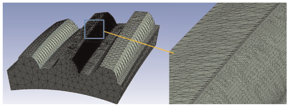
Finite element model of driving wheel

Figure 18.

Boundary conditions of gear pair.

When the mesh size of the contact tooth surface is changed from 0.15 to 0.1 mm, the maximum contact stress of the tooth surface changes from 763.02 to 763.11 MPa in Table 6 with a change rate of 0.09%. Therefore, the contact tooth surface mesh is individually encrypted to 0.15 mm to ensure the accuracy of contact stress simulation.

Table 6.

Mesh size and corresponding tooth surface maximum contact stress.

Tooth surface mesh size (mm)	Maximum contact stress value (MPa)
0.4	577.37
0.3	749.85
0.2	760.33
0.15	762.95
0.1	763.11

Referring to [29], the contact stress at the center of the tooth width of the bionic gear is analyzed. The contact stress nephograms of the driving and driven gears are depicted in Figure 19(a) and (b) when contacting at the center of the tooth width, respectively. The contact area is elliptical. Stress concentration occurs at the geometric mutation (tooth root). The maximum contact stress of 762.95 MPa occurs on the concave tooth surface of the driven gear in the contact area, indicating that the simulation results reflect the mechanical characteristics of the working bionic gear pair. After the tooth surface gradually runs in, the curvature radius of the contact arc between the convex and concave tooth surfaces tends to be equal, achieving the ideal situation of instantaneous contact along the tooth height line, which reduces the contact stress concentration.

(3) Contact curve length L of bionic gear

The gear contact curve length is mainly related to the spiral angle and module. Therefore, the control variable method is used to change the spiral angle and module of the bionic gear while keeping other parameters unchanged. A multi-group gear pair model is established, as depicted in Table 8. When the driven gear is fixed and the input torque is 1 × 10⁵ N.mm of the driving gear, the maximum contact stress of the tooth surface is $σ_{H}$ in equation (13). And the contact curve length L in equation (13) is derived. $σ_{H}$ and L are depicted in Table 7.

Table 7.

Different $σ_{H}$ and L under different gear parameters.

Group	Module m_n (mm)	Spiral angle β (°)	Artificial value $σ_{H}$ (MPa)	Length of contact curve L (mm)	Group	Module m_n (mm)	Spiral angle β (°)	Artificial value $σ_{H}$ (MPa)	Length of contact curve L (mm)
1	2	10	816.21	3.0247	11	6	10	420.32	3.8019
2		15	921.42	2.2549	12		15	515.50	2.4014
3		20	1152.40	1.3404	13		20	538.46	2.0465
4		25	1378.02	0.8522	14		25	574.77	1.6328
5		30	1531.68	0.6121	15		30	640.59	1.1664
6	4	10	538.81	3.4705	16	8	10	340.85	4.3361
7		15	615.83	2.5240	17		15	383.47	3.2548
8		20	698.74	1.8230	18		20	433.08	2.3727
9		25	772.61	1.3556	19		25	518.55	1.5046
10		30	841.56	1.0138	20		30	593.48	1.0192

Table 8.

Calculation parameters of bionic gear tooth root bending stress.

Parameters	Numerical value	Parameters	Numerical value
$H$	$h_{f} - r_{g 1}$	$S_{t}$	$(R - h_{f}) \cdot \sin θ_{a}$
$S_{h}$	0	$γ_{a}$	$asin (S_{t} / h_{f})$
$γ$	0	$γ_{t}$	$γ_{a} + θ_{a}$
$α$	0	$x_{f}$	$R \cos (θ_{a} / 2)$
$x_{t}$	$R - h_{f}$	$y_{f}$	$R \sin (θ_{a} / 2)$
$y_{t}$	0	$S_{f}$	$R \sin θ_{a}$
$θ_{a}$	$(1.54 m_{n} + j) / R$	$h_{F}$	$(R - S_{f} \tan θ_{0}) - S_{t} (1 / \tan θ_{a} - \tan γ_{a})$

Figure 19.

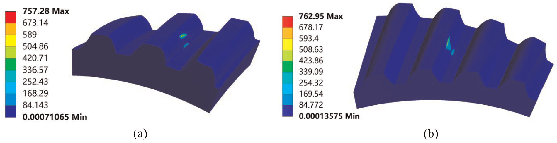
Equivalent stress nephogram of bionic gear: (a) The driving gear and (b) The driven gear.

The contact curve length L varying with the spiral angle and modulus is fitted by a polynomial as equation (14) shown.

\begin{matrix} L = 4.737 + 0.3523 m_{n} - 0.2714 β - 0.008303 m_{n}^{2} \\ - 0.006426 m_{n} β + 0.004246 β^{2} \end{matrix}

(14)

The formula for calculating the maximum contact stress of the bionic gear tooth surface is obtained by combining equations (13) and (14).

Bending strength of bionic gear

Mathematical model of tooth root bending stress of bionic gear

As depicted in Figure 20, the line m-m, perpendicular to the pitch line, passes through the center of the transition arc of the gear’s convex tooth profile. G point is the intersection point of the line m-m and the gear pitch line. o₂ point is the center of the transition arc of the convex tooth profile. A_G point is any point on the transition arc of the convex tooth profile. And A_G’ point is the connection point of the transition arc of the convex tooth profile and the root of the gear tooth. The distance between o₂ and the nodal line is H, and the distance between A_G and the nodal line m-m is S_h. The radius of the transition arc of the convex tooth profile is r_g₁, and the included angle between the line passing through A_G and o₂ and the nodal line is γ.

Figure 20.

Partial parameters of bionic gear tooth groove.

Equation (15) is deduced based on the geometric relationship.

{\begin{matrix} H = h_{f} - r_{g 1} \\ S_{h} = r_{g 1} \cos γ \end{matrix}

(15)

The bending stress of the convex tooth root is greater than that of the concave tooth root,³¹ so the maximum bending stress at the convex tooth root is selected for analysis. As depicted in Figure 21, the line passing through the center O and G points of the driving gear is the x-axis, the center of the gear circle is the coordinate origin, and the line perpendicular to the line OG is the y-axis. A_GB_G is the extension line of the line where the convex curve of the tooth profile transition arc curvature is located. The B_G point is on the pitch circle of the gear. α is the included angle between OB_G and the x-axis. The coordinate of A_G is (x_t, y_t). Since the included angle between the line m-m and the x-axis is small enough to be negligible, the line m-m and the x-axis are assumed to coincide.

Figure 21.

Tooth root position of bionic gear.

If y_t ≠ 0, the position of A_G on the transition arc of the convex tooth profile is:

{\begin{matrix} x_{t} = R \cos α - (R α + S_{h}) \frac{\sin (γ - α)}{\cos γ} \\ y_{t} = - R \sin α + (R α + S_{h}) \frac{\cos (γ - α)}{\cos γ} \end{matrix}

(16)

Where α = (H cotγ)/R, when y_t = 0, x_t = R−h_f .

As depicted in Figure 22(a), OO_Z is the center line of the tooth thickness of the gear teeth. A_GZ_G is the tangent line of the A_G point. γ_a is the included angle between the tooth thickness center line OO_Z and A_GZ_G. θ_a is the selected angle between OO_Z and the x-axis. C_G point is the center of the transition arc curve. p-p is the line through the B_G point, tangent to the pitch circle. n-n is the line where the direction of curvature is through the A_G point. A perpendicular line is drawn through the B_G point, perpendicular to the n-n line. Draw a perpendicular line through point C_G, intersecting at point D_G. The point of intersection point E_G of the line OD_G and the line n-n is the curvature center of the tooth root transition curve based on the Euler-Sauvard theorem.³¹ As depicted in Figure 22(b), S_t is the vertical distance from A_G point to OO_Z, the center line of the tooth thickness. h_F is the distance between two intersection points, A_G normal and the line OO_Z and k normal and the line OO_Z. The load application point k coordinates are (x_f, y_f).

Figure 22.

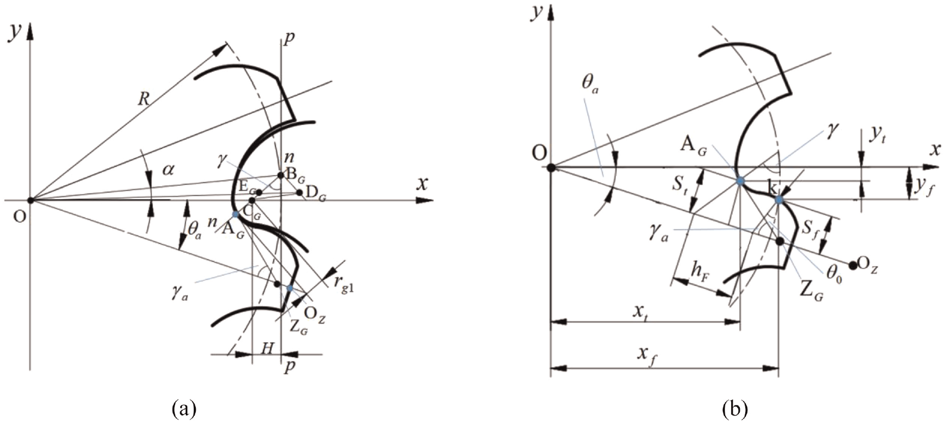
Convex tooth profile root analysis: (a) Meshing state and (b) Non meshing state.

Equation (17) is deduced based on the geometric relationship.

{\begin{matrix} θ_{a} = \frac{1.54 m_{n} + j}{2 π R} \\ γ_{a} = \arctan \frac{S_{t}}{h_{f}} \end{matrix}

(17)

Where, $S_{t} = \sqrt{{x_{t}}^{2} + {y_{t}}^{2}} \sin θ_{a}$ .

The load point coordinates of the convex tooth profile are:

{\begin{matrix} x_{f} = R \cos (θ_{a} / 2) \\ y_{f} = R \sin (θ_{a} / 2) \end{matrix}

(18)

As depicted in Figure 22(b), h_F is deduced as equation (19).

h_{F} = (R - S_{f} \tan θ_{0}) - S_{t} (1 / \tan θ_{a} - \tan γ_{a})

(19)

Where, $S_{f} = \sqrt{{x_{f}}^{2} + {y_{f}}^{2}} \sin θ_{a}$ .

H _a is deduced as equation (20).³⁰

H_{a} = \frac{- \cos γ_{a}}{2 [\frac{3 \frac{S_{t}}{ρ} + 2 \cos γ_{a}}{2 (\frac{S_{t}}{ρ})} + \frac{(\cos γ_{a} + \frac{S_{t}}{ρ})}{{(\frac{S_{t}}{ρ})}^{3}} \ln (\frac{\cos γ_{a}}{\cos γ_{a} + \frac{S_{t}}{ρ}})]}

(20)

$ρ$ is the curvature radius of the stress point on the transition curve of the tooth profile root. If $ρ = r_{g 1}$ , the equation of the tooth profile bending stress $σ_{0}$ is deduced as equation (21).

σ_{0} = F_{n} \cdot (\frac{\sin θ_{0} \cos^{2} γ}{2 S_{t}} - \frac{h_{F} \cos θ_{0}}{{S_{t}}^{2}} \cdot H_{a})

(21)

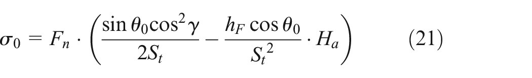
The maximum bending stress of the bionic gear tooth root occurs at the junction of the transition arc and the tooth root, which is the point A_G’ depicted in Figure 20. Therefore, the calculation parameters of the maximum bending stress at the root of the bionic gear are depicted in Table 8.

The designed bionic gear is a kind of helical gear with an asymmetric tooth shape, which is quite different from an involute spur gear. Therefore, the correction value $σ_{C}$ of tooth shape stress is added in equation (21). The mathematical model of the maximum bending stress of the bionic gear tooth root is deduced as equation (22) shown.

σ_{F} = σ_{0} + σ_{C} = F_{n} \cdot (\frac{\sin θ_{0} \cos^{2} γ}{2 S_{t}} - \frac{h_{F} \cos θ_{0}}{{S_{t}}^{2}} \cdot H_{a}) + σ_{C}

(22)

The mathematical expression of $σ_{C}$

Reference [31] shows that the spiral angle and modulus are important parameters of $σ_{C}$ in the design of a single circular arc gear. The control variable method is adopted to select 20 groups of bionic gear pair models in Table 9 for finite element analysis of bending stress in ANSYS software. When the driven gear is fixed and the input torque is 1 × 10⁵ N.mm of the driving gear, the maximum simulation value of tooth root bending stress $σ_{F}$ is subtracted from the theoretical stress value $σ_{0}$ to obtain $σ_{C}$ , as depicted in Table 9.

Table 9.

Bending stress analysis under different gear parameters.

Group	Module	Spiral angle β (°)	Simulation $σ_{F}$ (MPa)	Theoretical $σ_{0}$ (MPa)	Correction $σ_{C}$ (MPa)	Group	Module	Spiral angle β(°)	Simulation $σ_{F}$ (MPa)	Theoretical $σ_{0}$ (MPa)	Correction $σ_{C}$ (MPa)
1	2	10	157.93	149.7305	8.1995	11	6	10	45.88	49.9102	−4.0302
2		15	193.38	149.5996	43.7804	12		15	54.43	49.8665	4.5635
3		20	244.84	149.4181	95.4219	13		20	62.197	49.8060	12.4676
4		25	300.06	149.1181	150.9419	14		25	67.919	49.7294	18.1896
5		30	341.32	148.9118	192.4082	15		30	76.634	49.6373	26.9967
6	4	10	70.382	74.8653	−4.4833	16	8	10	34.926	37.4326	−2.5066
7		15	83.033	74.7998	8.2332	17		15	36.003	37.3999	−1.3969
8		20	99.936	74.7091	25.2269	18		20	39.602	37.3545	1.6031
9		25	116.89	74.5940	42.2960	19		25	44.843	37.2970	7.5460
10		30	131.61	74.4559	57.1541	20		30	48.972	37.2279	11.7441

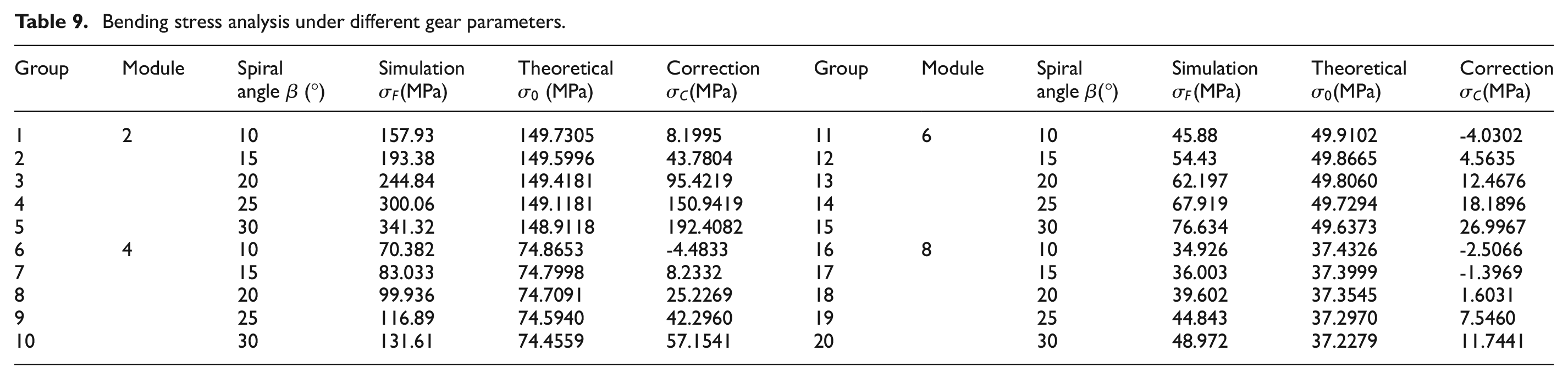
The tooth shape stress correction value $σ_{C}$ varying law with the spiral angle and modulus is polynomial fitted as equation (23).

\begin{matrix} σ_{C} = - 62.63 - 20.49 m_{n} + 14.66 β + 8.562 m_{n}^{2} - 3.824 m_{n} β \\ + 0.03064 β^{2} - 0.6114 m_{n}^{3} + 0.2416 m_{n}^{2} β - 0.001855 m_{n} β^{2} \end{matrix}

(23)

The formula for calculating the maximum bending stress of the bionic gear tooth root is obtained by combining equations (22) and (23).

Strength comparison between bionic gear and conventional gear

Strength comparison between bionic gear and involute helical gear

The teeth number, tooth width, helix angle, pressure angle, and modulus of the selected involute helical gear match those of the bionic gear in section “Research on the bionic gear tooth profile design.” For a more intuitive comparison of the strength of the involute helical gear and the bionic gear at different angular positions, the maximum contact stress and bending stress of the tooth root at different angles in the width direction are depicted in Figure 23(a) and (b), respectively.

Figure 23.

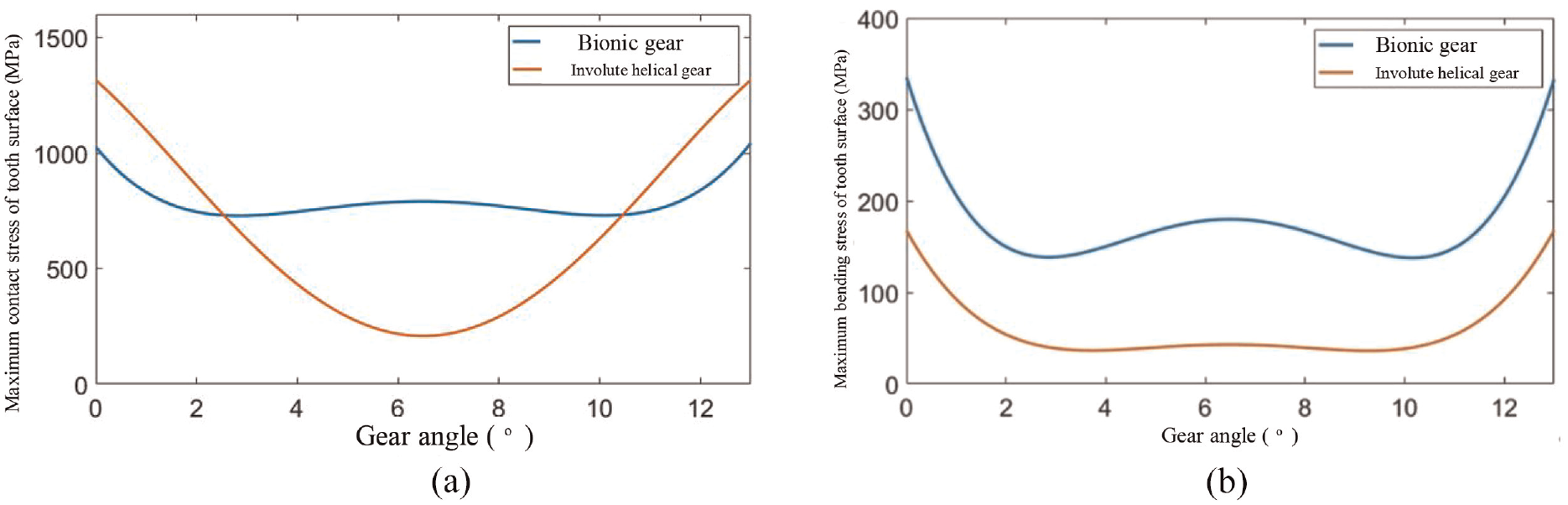
Comparison of contact and bending stress between bionic gear and involute helical gear at different angles in width direction: (a)The maximum contact stress and (b) The maximum bending stress.

It is depicted in Figure 23 as follows. (1) The involute helical gear is convex and convex profile meshing near the end face, while the bionic gear is convex and concave profile contact. The relative main curvature radius is different, so the maximum contact stress of the bionic gear tooth surface is small. The involute helical gear has a long contact line near the center of the tooth width, and the contact stress is distributed along the contact line. The bionic gear pair meshes at a point with a much smaller contact area than the line contact area. Therefore, the maximum contact stress of the involute helical gear tooth surface is smaller at the center of the tooth width. (2) Since the tooth height and root thickness of the bionic gear are smaller than those of the involute helical gear, the maximum bending stress of the bionic gear root is larger than that of the involute helical gear.

Strength comparison between bionic gear and pure rolling single arc gear

The teeth number, tooth thickness, tooth width, helix angle, pressure angle, and modulus of the pure rolling single arc gear are the same as those of the bionic gear in section “Research on the bionic gear tooth profile design.” To avoid the tooth profile interference of the single arc gear, the working profile radius of the convex gear is 4.5 mm,²⁴ and the working profile radius of the concave gear is 12 mm. For a more intuitive comparison of the strength of the single arc gear and the bionic gear at different angle positions, the maximum contact stress and bending stress of tooth root at different angles in the width direction are depicted in Figure 24(a) and (b), respectively.

Figure 24.

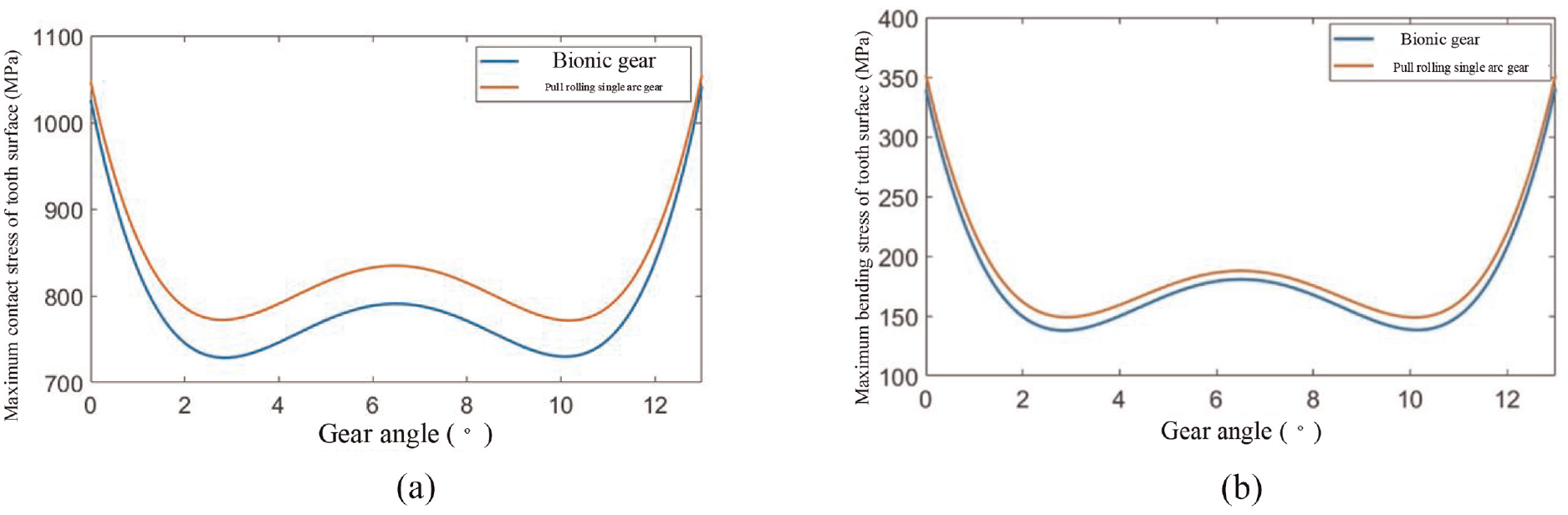
Comparison of contact and bending stress between bionic gear and single arc gear at different angles in width direction: (a)The maximum contact stress and (b) The maximum bending stress.

It is depicted in Figure 23 as follows. (1) The difference of the tooth profile curvature radius of the meshing bionic gear pair is smaller than that of the single arc gear pair to avoid the meshing interference, so the maximum contact stress of the bionic gear tooth surface is smaller than that of the single arc gear. (2) The thickness of the bionic gear root is larger than that of the single arc gear, so the maximum bending stress of the bionic gear root is smaller than that of the single arc gear.

Conclusions

Based on the requirements of the transmission efficiency and load capacity of the jumping robot transmission system, this paper analyzes the transmission characteristics of the planthopper hip joint gear. A bionic gear is designed based on the tooth shape and profile characteristics of the planthopper hip joint gear. The logarithmic spiral is taken as the working tooth profile of the bionic gear. The design method of the bionic gear is proposed. The transmission efficiency and error of the gear are analyzed. In addition, the theoretical formulas for the contact strength and bending strength of the bionic gear are deduced. The results show that the bionic gear is more suitable for the transmission system of high-performance jumping robots. (1) The transmission efficiency of bionic gears is 97.5%. The bionic gear rotates 360° with a transmission error of 25”. Its characteristics of small transmission error and high transmission efficiency meet the requirements of the jumping robot transmission system. (2) The maximum contact stress of the bionic gear tooth surface decreases by 29.8% compared with the involute helical gear. The relative sliding coefficient of the meshing pair is close to 0, which reduces the tooth surface damage and improves the load capacity. The tooth height of the bionic gear is more than twice as small as that of the involute gear, and the design of the teeth and tooth slots is more compact, which is helpful for the lightweight of the jumping robot. (3) Compared with the single arc gear, the maximum contact stress of the gear tooth surface decreases by 3.5%, and the maximum bending stress of the tooth root decreases by 2.1%. Meanwhile, the bionic gear requires only one tool during processing, which improves the process versatility and reduces the manufacturing cost.

Footnotes

Handling Editor: Chenhui Liang

Declaration of conflicting interests

The author(s) declared no potential conflicts of interest with respect to the research, authorship, and/or publication of this article.

Funding

The author(s) disclosed receipt of the following financial support for the research, authorship, and/or publication of this article: This work was partially supported by the National Natural Science Function of China (Grant no.51975500 and no.51975499). The authors would like to express their gratitude for the financial support.

ORCID iDs

Zenghuang He

Weixiong Ye

Data availability

The data used to support the findings of this study are available from the corresponding author upon request.

References

Liu

Jin

Jiang

, et al. Wheeled jumping robot by power modulation using twisted string lever mechanism. J Zhejiang Univ Sci A 2021; 22(10): 767–777.

Jung

Cho

KJ.

Froghopper-inspired direction-changing concept for miniature jumping robots. Bioinspir Biomim 201611(5): 056015.

Kovac

Fuchs

Guignard

, et al. A miniature 7g jumping robot. In: 2008IEEE international conference on robotics and automation, Pasadena, CA, USA, pp. 373–378.

Truong

Argyoganendro

Park

HC.

Design and demonstration of insect mimicking Foldable artificial wing using four-bar linkage systems. J Bionic Eng 2014; 11(3): 449–458.

Malcolm

Gregory

(2013). Interacting gears synchronize propulsive leg movements in a jumping insect. Science 2013; 341(6151): 1254–1256.

Shen

Qiao

Luo

, et al. Research on dynamic response characteristics and condition indicators of gear wear fault. Chin J Mech Eng 2021; 57(17): 120–131.

Liu

Meng

JL.

A novel non-involute gear designed based on control of relative curvature. Mech Mach Theory 2019; 140: 144–158.

Tan

Chen

Peng

, et al. Study on spatial curve meshing and its application for logarithmic spiral bevel gears. Mech Mach Theory 2015; 86: 172–190.

Zhao

XC.

Angular velocity and contact force simulation of the spiral bevel gear meshing based on the hertz contact theory. Eng Rev 2019; 2(39): 148–156.

10.

Yang

HC.

Investigation of a flea gear tooth modification. J Mech Sci Technol 2022; 36(3): 1209–1220.

11.

Liu

Stefanini

, et al. A novel bioinspired PVDF micro/nano hair receptor for a robot sensing system. Sensors 2010; 10: 994–1011.

12.

Geng

FZ.

Overview of high speed gear transmission technology and equipment. J Mech Trans (Chinese) 2019; 43(11): 172–175.

13.

Chen

XY.

Research and exploration of new energy vehicle drive motor selection. Auto Time 2023; 400(4): 101–103.

14.

Chang

Zhang

, et al. Establishment of the virtual prototype of angular transmission error of RV reducer based on multi-body dynamics simulation. Mech Trans (Chinese) 2018; 42(9): 168–172.

15.

Peng

Tang

Zhou

YS.

Considering the effect of shaft deformation for zero spiral bevel gear transmission error calculation. J Harbin Inst Technol 2019; 51(7): 121–127.

16.

Wang

Fan

Feng

The design methodology and characteristics analysis of a uniform-variable non-circular gear drive. Int J Interact Design Manufac 2019; 13(6): 821–830.

17.

State Bureau of Technical Supervision of the People’s Republic of China. Involute cylindrical gear accuracy. Beijing: Standards Press of China, 1988.

18.

Wang

Liu

XY.

The application of an edge detection algorithm in cephalopod beak recognition. Fishery Moderniz 2022; 49(4): 52–59+69.

19.

Dan

Liu

Gong

DF.

Smoothing filter detection algorithm based on middle and tail information of differential histogram. Comput Sci 2021; 48(11): 234–241.

20.

XT.

Principle of gear meshing. Xi’an: Xi’an Jiaotong University Press, 2009.

21.

Weng

Wang

GP.

Gearing theory and tooth area’s formation of logarithmic spiral bevel gear. J Liaoning Techn Univ (Natural Science) 2008; 27(1): 107–109.

22.

Guo

Qiao

Fan

, et al. Fan characteristic curve fitting based on Gaussian function and its application. Gold 2017; 38(4): 28–31.

23.

Liang

Chen

Gao

, et al. Generation principle and meshing characteristics of conjugate-curve circular arc gears. J Adv Mech Design Syst Manufac 2015; 9(1), JAMDSM0005.

24.

Wang

Chen

Zheng

, et al. A summary of research on effect of gear tooth root strengthening on bending fatigue strength based on residual stress. Mech Trans (Chinese) 2019; 43(12): 161–168.

25.

Zhao

Huang

JP.

Study on bending strength of pure rolling single arc gear. Mach Des Manufac 2019; 2020(9): 70–74.

26.

Chen

WH.

Preliminary differential geometry. Beijing: Peking University Press, 1990.

27.

Shao

JH.

Arc gear. Beijing: China Machine Press, 1994.

28.

Komori

Takeoka

, et al. Design and error analysis of multiball artifact composed of simple features to evaluate pitch measurement accuracy. J Mech Des 2009; 131(4): 041006.

29.

Chen

CW.

Failure characteristics and error effect of circular arc gear. Heavy Mach 1994; 5(5): 27–31.

30.

Wang

Root transition curve and root Stress. Beijing: National Defense Industry Press, 1989.

31.

Xia

Zhang

ZQ.

Finite element analysis on the bending stress of double circular arc gear with different load-on ways. New Technol New Proc 2009; 2009(03): 43–45.

Design and transmission performance analysis of planthopper hip joint gear

Abstract

Keywords

Introduction

Analysis of transmission characteristics of planthopper hip gear

Bionic design of planthopper hip gear

Analysis of tooth profile characteristics of planthopper hip gear

Mathematical properties of logarithmic spirals

Extraction and fitting of planthopper hip gear tooth

Research on the bionic gear tooth profile design

Construction of logarithmic spiral gear tooth shape of bionic gear

Design of logarithmic spiral tooth profile parameters for bionic gears

3D modeling of the bionic gear

Analysis of the transmission performance of bionic gear pair

Analysis of transmission efficiency and error of bionic gear pair

Analysis of transmission efficiency of bionic gear pair

Analysis of bionic gear transmission error

Contact strength analysis of bionic gear

Bending strength of bionic gear

Mathematical model of tooth root bending stress of bionic gear

The mathematical expression of σ C

Strength comparison between bionic gear and conventional gear

Strength comparison between bionic gear and involute helical gear

Strength comparison between bionic gear and pure rolling single arc gear

Conclusions

Footnotes

Declaration of conflicting interests

Funding

ORCID iDs

Data availability

References

The mathematical expression of $σ_{C}$