Sage Journals: Discover world-class research

Abstract

For the controller structure design problem, a controller design method based on the integration of structure search and parameter optimization is proposed with the idea of ENAS, which automates the controller structure design work, and searches for the most suitable controller structure and completes the parameter optimization in a relatively short time. The simulation study with the galvano scanner as the controlled plant shows that the number of iterations and the consumption time of the method are only 15% of the traditional method in achieving the same performance compared with the traditional design method.

Keywords

Structure search integrated design controller ENAS parameter optimization

Introduction

After years of theoretical research and engineering practice, a variety of structures and forms of control theory and its controller design methods have been created and developed. The construction of a new control system structure has been an important direction in the development of control theory and control engineering.

In actual engineering, the structure of the constructed control system will be more complex, as shown in Figure 1, which is the composition and principle diagram of a single-channel longitudinal electrotransmission manipulation system. The electrotransmission steering system is actually composed on the basis of control stabilization, eliminating the irreversible power-assisted mechanical steering channel and retaining only the channel of electrical command signal output from the driving rod via the rod force sensor. The function and control principle of the system is the same whether analog or digital. For each given aircraft there may be different system structure and functional requirements, that is, there are different control laws, but in the basic structure of the controller will be more or less the same.

Figure 1.

Composition and principle of single-channel longitudinal telegraphic manipulation system.¹

Therefore, for a control system used in engineering, its topology has a meaning and there exists a clear physical meaning and logical relationship. The development of traditional control system topology is also based on the continuous deepening of the mechanism of the controlled plant and control theory.

Most of the current control system optimization algorithms are for the optimization of control system parameters, control system structure optimization, or mainly rely on human intelligence and judgment.

Zoph and Le proposed a Neural Architecture Search (NAS) method to find a suitable neural network structure in 2017.² They used an RNN generator sampling to obtain a new neural network structure. The data is trained under this neural network structure and the accuracy on the corresponding validation set is obtained. This accuracy is used to characterize the performance of the neural network obtained from this search, which is then used as a reward function to train the RNN generator. The conceptual structure is shown in Figure 2.

Figure 2.

NAS basic framework.²

Since NAS methods consume a lot of computational resources, Pham et al. proposed an Efficient Neural Architecture Search (ENAS) method to quickly design the structure and weights of neural networks based on NAS.³ It uses an LSTM (Long Short-Term Memory) as a generator to express the network structure as a directed acyclic graph. The directed acyclic graph has edges and nodes, where each node represents an operation and the edges represent the information flow. ENAS trains a generator to select an optimal subgraph from the directed acyclic graph (which determines which edges are activated in the directed graph), while the selected subgraph is trained using the classical Cross Entropy Loss.

Some specific applications of structure search have already emerged. Luo used NAS to compress large scale pre-trained language model and text-to-speech model by proposing or utilizing block-wise training, progressive pruning and performance approximation.⁴ Zhou combined Huffman coding with NAS algorithm and applied it to image segmentation task.⁵ Luo proposed an efficient NAS algorithm by combining Dynamical Isometry and achieve an high accuracy rate on the ImageNet classification task.⁶ To overcome the ENAS model generalization error problem, Ahmed et al. examined the effectiveness of a range of techniques including reducing model complexity, use of data augmentation, and use of unbalanced training sets, and achieved remarkable results on the ultrasound image classification for breast lesions.⁷

Although the ENAS method was proposed for designing the structure and weights of neural networks,³ the idea of ENAS can be extended to design the structure and edge weights of any directed acyclic graph. Since the control system (CS) can be transformed into the form of a directed acyclic graph, this paper draws on the idea of ENAS to design the structure and parameters of the control system (CS) in an integrated manner, as shown in Figure 3.

Figure 3.

The basic framework of the methodology in this paper.

In this paper, a controller design method based on the integration of structure search and parameter optimization is proposed to automate the controller structure design. The method introduces the idea of ENAS, which can search for the most suitable controller structure and complete parameter optimization in a relatively short time. In this paper, the galvano scanner in Maeda and Iwasaki’s paper⁸ is selected as the research plant to verify the effectiveness of the method and compare it with the traditional full search-based method.

Controller structure automatic generation technology

Conversion method of control law and control system structure diagram

The central scientific and technical problem of this section is to transform the control system structure into a directed acyclic graph structure that the LSTM can handle.

A complex system structure diagram, the connection between its boxes is bound to be intricate, but the only three basic ways to connect the boxes are series, parallel and feedback connections. Therefore, the general method of simplifying the structure diagram is to move the lead or comparison points, exchange the comparison points, and perform box operations to merge the boxes connected in series, parallel and feedback. The principle of maintaining equivalent variable relationships before and after the transformation should be followed in the simplification process. Eventually, the structure of all closed-loop control systems can be expressed in the form of Figure 4.

Figure 4.

Classic FB control system block diagram.⁹

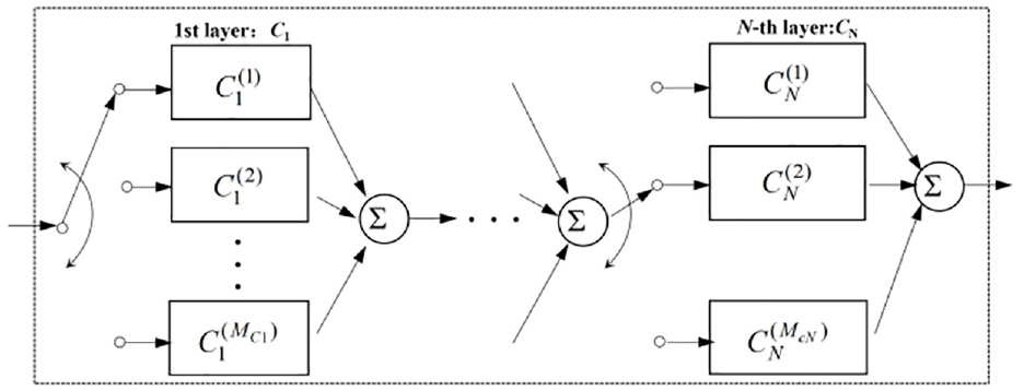
where $C (s)$ is the controller transfer function. The transfer function $C (s)$ is set to the N-layer structure controller as shown in Figure 5 (any controller can be written in the form of N transfer functions multiplied by each other).

Figure 5.

N-layer cascade structure controller block diagram.¹⁰

Since the controller is a cascade structure, the transfer function $C (s)$ is

C (s) = Π_{i = 1}^{N} C_{i} (s)

Here $C_{i} (s)$ denotes a transfer function picked from the ith layer, that is, the transfer function of the connected part of each layer in Figure 5. Each $C_{i} (s)$ can be set to the following form.

C_{i} (s) = {\begin{matrix} a_{0 i}^{(1)} \\ \frac{a_{1 i}^{(2)} s + a_{0 i}^{(2)}}{b_{1 i}^{(2)} s + b_{0 i}^{(2)}} \\ \frac{a_{2 i}^{(3)} s^{2} + a_{1 i}^{(3)} s + a_{0 i}^{(3)}}{b_{2 i}^{(3)} s^{2} + b_{1 i}^{(3)} s + b_{0 i}^{(3)}} \\ ⋮ \\ \frac{a_{ni}^{(n + 1)} s^{n} + \dots + a_{1 i}^{(n + 1)} s + a_{0 i}^{(n + 1)}}{b_{ni}^{(n + 1)} s^{n} + \dots + b_{1 i}^{(n + 1)} s + b_{0 i}^{(n + 1)}} \end{matrix}

The transfer function can be decomposed into the form of the product of N transfer functions according to the above method.

Structural modeling of control systems based on directed acyclic graphs

As mentioned above, an arbitrary controller can be written in the form of N transfer functions multiplied by each other. Further, we can convert the cascaded structure controller shown in Figure 5 into a directed acyclic graph, as shown in Figure 6, for comparison with the graph defined by Pham et al.,³ following the following steps:

Step 1 Define each box of the controller structure diagram as a node.

Step 2 Which edge is activated: each edge in the controller structure graph is activated.

Step 3 What is the operation of a node: The operation of a node is a certain controller that is selected.

Figure 6.

Controller structure diagram.

Based on the above steps, the controller can be completely transformed into a directed acyclic graph. Then, the structure of this directed acyclic graph can be searched/optimized by the ENAS method.

Note that, as shown in Figure 6, we only convert the controller to a directed acyclic graph, while for the whole control system, it remains a directed cyclic graph structure.

Method for encoding topological relations of directed acyclic graphs

The encoding method for the topological relations of a directed acyclic graph as shown in Figure 6 is to generate an N-dimensional vector

(\begin{matrix} x_{1} & x_{2} & \dots & x_{i} & \dots & x_{N} \end{matrix})

Where $x_{i} \in {1, 2, \dots, M_{C_{i}}}$ and $M_{C_{i}}$ is the number of candidate structures for the i-th layer controller.

Thus, the number of all possible controller structures in the search space represented by this graph is $M_{C_{1}} \times M_{C_{2}} \times \dots \times M_{C_{N}}$ .

For example, the whole control system is 4-layer, if the diagram code is (1 3 2 2), it means that the first structure is selected for the first layer, the third structure is selected for the second layer, the second structure is selected for the third layer, and the second structure is selected for the fourth layer, as shown in Figure 7.

Figure 7.

Example of diagram coding.

Controller design rules embedding method

As mentioned above, the transfer function of the controller can be decomposed into the form of a product of N transfer functions. Further, each part can be considered as a filter, and the design of the controller is actually the design of N filters. When designing a circuit for a filter, it is difficult to directly implement a circuit with a transfer function of order 3 or higher. When it is necessary to design a filter greater than or equal to 3rd order, it generally takes the form of decomposing the higher-order transfer function into the product of several lower-order transfer functions. For example, to design a 5th-order filter, two 2nd-order filters and a 1st-order filter cascade can be obtained. Common filters are: low-pass filter, high-pass filter, band-pass filter, band-stop filter (notch filter), all-pass filter, etc., as shown in Table 1.

Table 1.

Transfer function of typical filters.

Type	$G (s)$
1st-order LPF	$\frac{G_{0} ω_{c}}{s + ω_{c}}$
1st-order HPF	$\frac{G_{0} s}{s + ω_{c}}$
1st-order APF	$\frac{G_{0} (s - ω_{c})}{s + ω_{c}}$
2nd-order LPF	$\frac{G_{0} ω_{n}^{2}}{s^{2} + 2 ζ ω_{n} s + ω_{n}^{2}}$
2nd-order HPF	$\frac{G_{0} s^{2}}{s^{2} + 2 ζ ω_{n} s + ω_{n}^{2}}$
2nd-order BPF	$\frac{2 ζ G_{0} ω_{0} s}{s^{2} + 2 ζ ω_{0} s + ω_{0}^{2}}$
2nd-order BSF(NF)	$\frac{G_{0} (s^{2} + ω_{0}^{2})}{s^{2} + 2 ζ ω_{0} s + ω_{0}^{2}}$
2nd-order APF	$\frac{G_{0} (s^{2} - 2 ζ ω_{0} s + ω_{0}^{2})}{s^{2} + 2 ζ ω_{0} s + ω_{0}^{2}}$

For the actual plant to be controlled, determining the number and type of filters, etc. requires the use of rules and a priori knowledge from the controller design domain. At this point, we can embed these rules and a priori knowledge by adjusting the parameter range. For example: by analyzing the bode plot of the controlled plant, it is found that there are two wave peaks to be handled, we can set the number of filters as 2 and the frequency selection range of the filters as the periphery of the two wave peak positions respectively; according to the a priori knowledge, the improvement of the controller performance may require band-stop filters or all-pass filters, then the filters can be designed as

\frac{G_{0} (s^{2} + 2 ζ_{1} ω_{0} s + ω_{0}^{2})}{s^{2} + 2 ζ_{2} ω_{0} s + ω_{0}^{2}}

The change from BSF to APF can be achieved by first fixing $ζ_{2}$ so that $ζ_{1}$ varies between $- ζ_{2}$ and $ζ_{2}$ .

Automatic controller parameter optimization technique based on efficient heuristic search algorithm

General topology study of control systems

The structure of the controller varies significantly depending on the control theory on which the controller is based, and it is often very complex in engineering because of the need to solve various characteristic problems and constraint problems of the controlled plant. Based on this, we adopted the expression of a cascade controller. After analysis, it is believed that the classical multi-loop control systems and control laws can be basically transformed into this form.

In addition, for the actual control system, there are multiple high-frequency resonant mode disturbances in addition to the nonlinear characteristics. Therefore, when designing a controller, a basic controller is generally designed for completing the stability control, and then multiple filters are designed for each resonant mode to improve the overall performance of the controller. As shown in Figure 8. The basic controller can use PID controller, robust controller, LQR controller, sliding mode controller, etc.

Figure 8.

Common topology for controller.

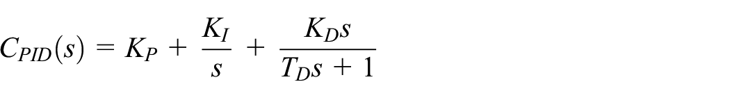
For example, the basic controller uses a PID controller and there are two resonant modes that need to be filtered, when C(s) can be designed as a cascade structured FB controller using a PID controller for the rigid mode and two second order filters for the first and second resonant modes. the mathematical expression of C(s) in the continuous time domain is defined by the following equation.

C (s) = C_{PID} (s) Π_{i = 1}^{2} C_{Fi} (s)

C_{PID} (s) = K_{P} + \frac{K_{I}}{s} + \frac{K_{D} s}{T_{D} s + 1}

C_{Fi} (s) = \frac{s^{2} + 2 ζ_{Fni} ω_{Fi} s + ω_{Fi}^{2}}{s^{2} + 2 ζ_{Fdi} ω_{Fi} s + ω_{Fi}^{2}}

Filter structure design method

Taking into account the study of controller topology and the control law design domain rule embedding method this paper adopts the structure of multiple filters cascaded with three possible forms for each filter, as shown in Figure 9.

Figure 9.

The filter structure in this paper.

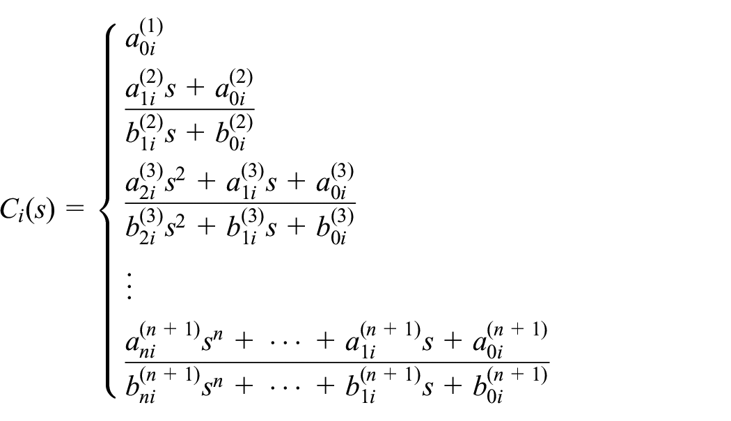
where the transfer functions of the three filters are:

(1) 0-order filter: $1$

(2) 1st-order filter:

\frac{s + ζ_{Fni} ω_{Fi}}{s + ω_{Fi}}

(3) 2nd-order filter:

\frac{s^{2} + 2 ζ_{Fni} ω_{Fi} s + ω_{Fi}^{2}}{s^{2} + 2 ζ_{Fdi} ω_{Fi} s + ω_{Fi}^{2}}

It can be seen from the transfer functions of the three filters: the 0-order filter is equivalent to an all-pass filter with no change in phase; the 1st-order filter varies between an all-pass filter and a high-pass filter as $ζ_{Fni}$ varies; the 2nd-order filter varies between an all-pass filter, a band-stop filter and a band-pass filter as $ζ_{Fni}$ and $ζ_{Fdi}$ vary.

Controller parameter optimization method

After obtaining the structure and initial parameters of the controller, it is necessary to substitute this controller and parameters into the closed loop of the whole system, and to adjust and optimize the parameters of the controller.

In the control system shown in Figure 4, $C (s)$ is defined as a cascade structure controller with a basic controller $C_{base} (s)$ and N filters $C_{Fi} (s)$ connected in series:

C (s) = C_{base} (s) Π_{i = 1}^{N} C_{Fi} (s)

The design problem of $C (s)$ is to obtain all controller parameters $η_{C}$ that can maximize the control bandwidth while satisfying the specified gain margin $g_{m}$ and phase margin $ϕ_{m}$ . The controller parameter $η_{C}$ is divided into two parts: the basic controller parameters $η_{base}$ and the other parameters $η_{other}$ .⁹

η_{C} = {η_{base}, η_{other}}

η_{other} = {ω_{F 1}, ζ_{Fn 1}, \dots, ω_{FN}, \dots}

The controller design method based on hybrid optimization uses different optimization methods to obtain the parameters of the cascade structure controller for the above two parts of the parameters, respectively. For the basic controller parameter $η_{base}$ , the theory and method related to the basic controller are used to tune the controller parameters; while for the other parameters $η_{other}$ , the GA-based optimization method is used to tune the parameters. The detailed design process is as follows:

Step 1 Randomly generate the initial population $η_{other}$ (population size $N_{pop}$ ) as the first generation ( $i_{pop}$ =1).

Step 2 Obtain the parameters $η_{base}$ of $N_{pop}$ candidates applicable to $η_{other}$ by this basic controller related theory and method.

Step 3 According to the defined fitness function (which reflects the control bandwidth and stability margin), the fitness scores $f$ of all individuals are evaluated in the GA using $η_{base}$ and $η_{other}$ to obtain the elite individuals.

Step 4 If the generated $i_{pop}$ is less than the specified number $N_{\max}$ , then $i_{pop} = i_{pop} + 1$ and go to step 5; otherwise, go to step 6.

Step 5 Perform genetic operations, such as selection, crossover and mutation, and generate a new population $η_{other}$ for the next generation. repeat steps 2∼5 when $i_{pop} \leq N_{\max}$ .

Step 6 Use the elite $η_{base}$ and $η_{other}$ to obtain the desired $C (s)$ , which extends the control bandwidth while satisfying a specific stability margin.

Selection of the fitness function and determination of important parameters

The most important requirement of the control system is fast and accurate, which requires the bandwidth to be as high as possible, but too much bandwidth can lead to system stability degradation, so the fitness (reward) function is selected considering both high bandwidth and sufficient stability margin, and we have determined the following forms of fitness functions:

(1) Summation type

F (i) = ω_{b} + g_{m} + ϕ_{m}

where $ω_{b}$ is the bandwidth (in rad/s), $g_{m}$ is the gain margin, and $ϕ_{m}$ is the phase margin (in degrees).

(2) Additional bonus type

F (i) = ω_{b} + g_{m} + ϕ_{m} + c_{1} R_{g_{m}} + c_{2} R_{ϕ_{m}}

c_{1} = {\begin{matrix} 1, g_{m} > 5 \\ 0, g_{m} \leq 5 \end{matrix}

c_{2} = {\begin{matrix} 1, ϕ_{m} > 30 \\ 0, ϕ_{m} \leq 30 \end{matrix}

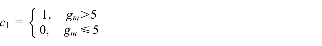
where 5 and 30° are referenced from the literature.⁹ $R_{g_{m}}$ and $R_{ϕ_{m}}$ are additional bonus values for gain margin and phase margin, respectively, which can be adjusted.

(3) Feasible domain type

F (i) = {\begin{matrix} ω_{b} + g_{m} + ϕ_{m}, g_{m} > 5 and ϕ_{m} > 30 \\ 0, else \end{matrix}

The direct summation-type fitness function focuses too much on the bandwidth and ignores the gain margin and phase margin, and from the simulation results, the system is in the edge of stability in most cases. The feasible domain adaptability function varies too much in the feasible domain edge function value, which is easy to fall into the local optimum and not easy to find a better solution. By adjusting the extra reward value, the local optimal solution can be gradually transitioned to a better solution through genetic iteration. The extra reward value cannot be too large, which will lead to a local optimum, or too small, which will make the fitness function focus too much on bandwidth and ignore the system stability. Therefore the extra reward equation is a form of fitness function between the direct summation equation and the feasible domain equation. The actual reward value needs to be finally determined by repeated experiments.

The larger the number of populations in the genetic algorithm, the better the population diversity and the higher the probability of convergence to the global optimal solution, but the more computational resources are consumed. Taking into account the convergence of the genetic algorithm and the time overhead of the computational process, the number of populations in the genetic algorithm is set to 50, the number of elites is set to 7, the number of crossovers is set to 40, the number of variants is set to 3, the number of iterations is set to 2000, and other default settings are used.

Lightweight and efficient search method for overall optimization of controller structure and parameters

Design of LSTM networks

Following the ENAS approach proposed by Pham, the LSTM samples the decisions in an autoregressive manner by means of a Softmax classifier: the decisions from the previous step are embedded as inputs to the next step. In the first step, the controller network receives the empty embedding as an input. For the control system, what needs to be determined is the number of filters and the order of each filter. The number of filters generally depends on the needs of the actual problem.

The filters are divided into 0-order, 1st-order, and 2nd-order, so the number of output categories of LSTM is 3. Assuming that the number of filters is N, as in Pham et al.’s original paper,³ the input size of LSTM is 1, and the length of the input stream is N, which denotes N filters, respectively. As shown in Figure 10(a) represents the sampled output results of the LSTM recurrent cell, and (b) represents the filter structure corresponding to the output of the LSTM recurrent cell. Note that the input of the initial recurrent cell is 0 and the output is 3-category probability. After sampling out the first filter structure as a 1st order filter, this is used as the input to transmit to the recurrent cell, and then the 3rd-order filter is sampled from the output of the 3-category probability, and so on.

Figure 10.

An example of an LSTM recurrent cell: (a) the sampled output results of the LSTM recurrent cell and (b) the filter structure corresponding to the output of the LSTM recurrent cell.

Pham et al. used an LSTM with 100 hidden units in the original paper.³ Comparing the size of the problem in this paper with Pham et al.’s paper, we use an LSTM with 10 hidden units.

Overall training scheme for controller structure search and parameter optimization

Throughout the training process, there are two sets of learnable parameters: the parameters of the LSTM are denoted by $θ$ , and the shared parameters of the filter are denoted by $ω$ . The training process consists of two interleaved phases. The first stage trains the shared parameters of the filter, $ω$ , and optimizes the parameters from the whole by genetic algorithm. In the actual experiment, the number of training steps per round of $ω$ is set to 20 (taking into account the convergence of the genetic algorithm and the time overhead of the computational process, the number of iterations per round of training of the genetic algorithm is set to 20). The second stage trains the parameters of the LSTM $θ$ . Unlike the original ENAS paper, where the object of study is the data set and multiple sets of data need to be sampled for updating, the object of study in this part is a single controlled system, which is set to perform one parameter update in the actual experiment. These two phases are alternated during the training process, and the total number of rounds is generally set between 100 and 200. More details are as follows.

Train the filter with shared parameters $ω$

In this step, fix Generator’s policy $π (m; θ)$ and perform genetic iterations on $ω$ to maximize the fitness function $F (i)$ . The filter structure $M$ is sampled from $π (m; θ)$ . We can use any individual model $M$ sampled from $π (m; θ)$ to update $ω$ . As mentioned before, we train $ω$ throughout the process of finding a better value of the fitness function.

Train the generator parameters $θ$

In this step, fix $ω$ and update the policy parameters $θ$ with the goal of maximizing the desired fitness $E_{m ~ π (m; θ)} [F (m, ω)]$ . We use the SGDM or Adam optimizer, for which the gradient is computed using the classical REINFORCE algorithm in reinforcement learning, and a sliding average baseline to reduce the variance. The fitness $F (M, ω)$ is computed by imposing the controller on the target plant to encourage the selection of a well-performing controller structure. The sliding average baseline is given by:

b = dec \times b + (1 - dec) \times coe \times F (m, ω)

Where $dec$ is the sliding ratio, taken as 0.9; $coe$ is the coefficient of the fitness function, taken as 0.001, because the fitness is generally greater than 10³; and the initial value of $b$ is taken as 0.

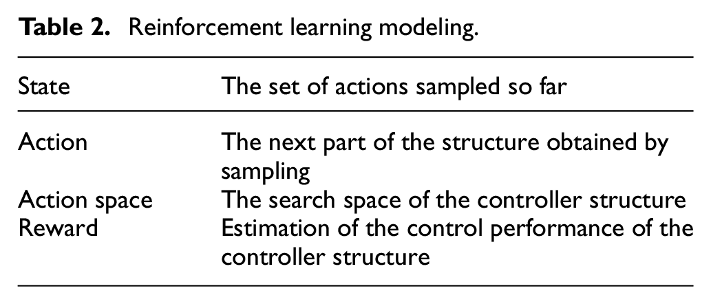
In order to model the problem as a reinforcement learning problem, it can be assumed that the generation of the controller structure is the action of an agent whose action space is the same as the search space of the controller structure. The “reward” of the agent is based on the estimation of the control performance of the controller structure. The policy samples various “actions” to sequentially generate the controller structure, and the “state” of the environment consists of the set of actions sampled so far, and is rewarded only after the final action. As shown in Table 2.

Table 2.

Reinforcement learning modeling.

State	The set of actions sampled so far
Action	The next part of the structure obtained by sampling
Action space	The search space of the controller structure
Reward	Estimation of the control performance of the controller structure

Determining the optimal architecture and parameters

After the overall training for controller structure search and parameter optimization, we first select the controller structure with the highest probability from the trained strategy $π (m, θ)$ . Then we take only the model parameter $ω$ with the highest adaptation from the shared parameters.

The whole process is shown in Figure 11.

Figure 11.

Training framework.

Selection of the optimizer and determination of important parameters

Currently, the mainstream optimizers are stochastic gradient descent (SGD),¹¹ momentum stochastic gradient descent (SGDM),¹² adaptive gradient descent (Adagrad),¹³ root mean square propagation optimization (RMSProp),¹⁴ and adaptive moment estimation optimization (Adam).¹⁵

The five major optimizers are actually divided into two categories, SGD, SGDM, and Adagrad, RMSProp, Adam. the more used ones are SGDM and Adam. as shown above, SGDM is more used inside computer vision (CV), while Adam basically sweeps natural language processing (NLP), reinforcement learning (RL), generative adversarial networks (GAN), and Speech synthesis and other fields. For example, in the field of NLP, the classical models Transformer and BERT all use Adam, and its variant AdamW.

In this paper, the controller structure is generated in LSTM, which is different from all of the above application areas and requires several experiments to determine the specific problem. The LSTM can be trained with input weights, recurrent weights and bias parameters. The input weights are initialized using the Glorot initializer (also known as the Xavier initializer). The Glorot initializer samples independently from a uniform distribution with mean zero and variance 2/(inputsize+numout) (inputsize for this part of the LSTM is 1), where numout = 4* numhiddenunits. For the initialization of the cyclic weights the orthogonal matrix Q given by the QR decomposition of the random matrix Z sampled from the unit normal distribution is used. For the bias, we use 1 to initialize the oblivious gate bias and 0 for the rest of the bias.

Simulation example

Target plant

This example draws on the laboratory galvano scanner of the laser processing machine in Makoto Iwasaki’s paper as the target plant under control. The galvano scanner consists of a rotating motor, a mirror, and an optical encoder, and fast response and high-precision control of the motor angle is required to achieve high productivity in high-density interconnect (HDI) printed circuit boards.

The mathematical model used in this example is structurally typical in that it can simulate both delay characteristics and high frequency disturbances. It has a primary resonant mode of 2960 Hz and a secondary resonant mode of 6100 Hz. The transfer function of the system is as follows:

P (s) = e^{- Ls} K_{p} (\frac{1}{s^{2}} + \sum_{i = 1}^{2} \frac{k_{i}}{s^{2} + 2 ζ_{i} ω_{i} s + ω_{i}^{2}})

The parameters are shown in Table 3.

Table 3.

Parameters of the target plant model.

$L$	1.9 × 10⁻⁵
$K_{p}$	1 × 10⁶
$k_{1}$	0.41
$k_{2}$	−1.65
$ω_{1}$	2 $π$ × 2960
$ω_{2}$	2 $π$ × 6100
$ζ_{1}$	0.004
$ζ_{1}$	0.015

Its Bode plot is shown in Figure 12.

Figure 12.

Bode plot of the target plant.

Filter structure design

This example uses a structure with two filter cascades, each with three possible forms, for a total of nine possible structures, as shown in Figure 13. The basic controller uses a PID controller with a low-pass filter with a transfer function of the form:

C_{PID} (s) = K_{P} + \frac{K_{I}}{s} + \frac{K_{D} s}{T_{D} s + 1}

Figure 13.

The filter structure used in this example.

Therefore, the basic controller parameters $η_{base}$ for this example are $η_{PID}$ , including $K_{P}$ , $K_{I}$ and $K_{D}$ , and the other parameters $η_{other}$ including $T_{D}$ , $ω_{F 1}$ , $ζ_{Fn 1}$ , $ζ_{Fd 1}$ , $ω_{F 2}$ , $ζ_{Fn 2}$ , $ζ_{Fd 2}$ . The range of parameters $η_{other}$ for the other parameters is shown in Table 4.

Table 4.

Parameter range of $η_{other}$ .

Parameters	Min.	Max.
$T_{D}$	1 × 10⁻⁴	1 × 10⁻⁴
$ω_{F 1}$	2 $π$ × 1000	2 $π$ × 2960
$ζ_{Fn 1}$	−1	1
$ζ_{Fd 1}$	0	1
$ω_{F 2}$	2 $π$ × 5965	2 $π$ × 12,000
$ζ_{Fn 2}$	−1	1
$ζ_{Fd 2}$	0	1

From Tables 3 and 4, it can be seen that the first filter is mainly for the first resonant mode and the second filter is mainly for the second resonant mode. From the transfer functions of the three filters, it can be seen that: the zero-order filter is equivalent to an all-pass filter with no phase change; the first-order filter varies between an all-pass filter and a high-pass filter as $ζ_{Fni}$ changes; the second-order filter varies between an all-pass filter, a band-stop filter (trap filter) and a band-pass filter as $ζ_{Fni}$ and $ζ_{Fdi}$ change. In addition, since the parameter $T_{D}$ is independent of the filter structure, $T_{D}$ is fixed to 1 × 10⁻⁴ for the convenience of comparing and analyzing the simulation results of full-search and structure search.

Hybrid optimization-based controller design method and selection of fitness function

From the analysis in previous section it can be seen that the parameters to be optimized are $η_{PID}$ and $η_{other}$ . Among them, $η_{PID}$ uses MATLAB’s own function “pidtune” for parameter tuning, while the parameter tuning of $η_{other}$ is carried out using a genetic algorithm GA. The detailed design process is as follows:

Step 1 Randomly generate the initial population $η_{other}$ (population number $N_{pop}$ ) as the first generation ( $i_{pop} = 1$ ).

Step 2 Obtain the PID parameters $η_{PID}$ applicable to the candidate of population $N_{pop}$ of $η_{other}$ by the pidtune function, which can automatically adjust the controlled objects under the specified phase margin according to the user requirements (signal tracking, interference suppression).

Step 3 According to the defined fitness function, the fitness scores $f$ of all individuals are evaluated with $η_{base}$ and $η_{other}$ to obtain the elite parameters $η_{other}$ for elite individuals.

Step 4 If the generated $i_{pop}$ is less than the specified number $N_{\max}$ , then $i_{pop} = i_{pop} + 1$ and go to step 5; otherwise, go to step 6.

Step 5 Perform genetic operations, such as selection, crossover and mutation, and generate a new population $η_{other}$ for the next generation. then $i_{pop} \leq N_{\max}$ . Repeat steps 2∼5.

Step 6 Use elites $η_{base}$ and $η_{other}$ to obtain the desired $C (s)$ . This extends the control bandwidth while meeting specific stability margins.

Based on iterative experiments, the final fitness function is determined as:

F (i) = ω_{b} + g_{m} + ϕ_{m} + 4000 c_{1} + 4000 c_{2}

c_{1} = {\begin{matrix} 1, g_{m} > 5 \\ 0, g_{m} \leq 5 \end{matrix}

c_{2} = {\begin{matrix} 1, ϕ_{m} > 30 \\ 0, ϕ_{m} \leq 30 \end{matrix}

Design of LSTM networks and selection of optimizers

For the controlled object of this example, the number of filters is determined to be 2, and what needs to be determined is the order of the two filters.

The number of output categories of the LSTM is 3, representing three filters. the input size of the LSTM is 1, and the length of the input stream is 2, representing two filters respectively. The number of hidden cells is 10. The network architecture is shown in Figure 14.

Figure 14.

The architecture of this LSTM.

Figure 15 shows an example where (a) represents the filter structure corresponding to the output of this LSTM recurrent cell, and (b) indicates that the sampled output results of this LSTM recurrent cell.

Figure 15.

An example of this LSTM recurrent cell: (a) the sampled output results of this LSTM recurrent cell and (b) the filter structure corresponding to the output of this LSTM recurrent cell.

For the optimizer, the learning rate is experimentally found to be the key parameter. Too high a learning rate will lead to too fast convergence, and the Generator may not search sufficiently for various structures and may even converge to non-optimal structures; too low a learning rate will lead to insignificant convergence. To achieve a lightweight optimizer, the SGDM is modified as follows, drawing on Adam’s idea:

learnRate = \frac{initialLearnRate}{1 + decay \times iteration}

The decay of the learning rate is linked to the number of iterations, which not only realizes the adaptive update of the learning rate, but also makes the decay process of the learning rate smoother. After several experiments, the initial learning rate initialLearnRate is taken as 0.003 and the decay rate decay is taken as 0.01.

Results

Set the number of LSTM network update iterations to stop when a certain structure reaches 100 first. The results are as follows:

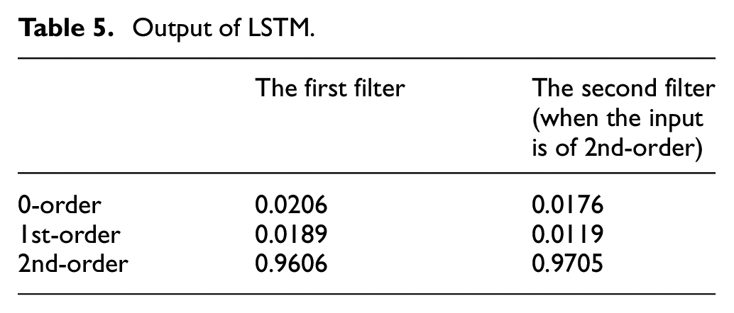
As can be seen in Figure 16, the filter structure converges to the 2nd order-2nd order form. the output of the LSTM is shown in Table 5. Figure 17 shows the comparison of the Bode plot before and after filtering, where SG1 and SG2 denote the sensitivity gain at the two resonant frequencies, respectively, and it can be seen that the first resonance frequency has a significant decrease in sensitivity, while the second resonance frequency has a small decrease in sensitivity.

Figure 16.

Simulation results: (a) number of iterations per structure, (b) loss function with baseline, (c) output of the first time step of the LSTM, and (d) output of the second time step of the LSTM.

Table 5.

Output of LSTM.

	The first filter	The second filter (when the input is of 2nd-order)
0-order	0.0206	0.0176
1st-order	0.0189	0.0119
2nd-order	0.9606	0.9705

Figure 17.

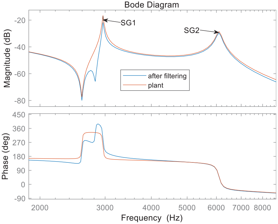
Comparison of Bode plot before and after filtering.

For comparison, the conventional exhaustive method was used for the experiments, and the results are shown in Table 6. It can be seen that: (1) The optimal structure form is PID-2nd-2nd; (2) The structure of the first filter is critical to the system bandwidth; (3) The controller structure search and parameter optimization method used in this example can effectively converge to the optimal structure, and the control performance is close to the optimal control performance of the full-search method; (4) Compared to the full-search method, the number of iterations and the time consumed by the method used in this example is only 15%.

Table 6.

Comparison of simulation results of two methods.

Method	Structure	BW (rad/s)	GM	PM (deg)	Fitness	SG1 (dB)	SG2 (dB)	Iteration number
Full-search	PID-0-0	887.8	0.06	71.7	4959.56	0	0	18,000
	PID-0-1st	1464.0	7.6	59.3	9530.9	−5.6	−2.9
	PID-0-2nd	1705.3	7.3	59.4	9772.0	0.4	2.1
	PID-1st-0	1762.6	5.5	64.6	9832.7	−0.8	−0.2
	PID-1st-1st	2091.5	7.8	59.4	10,158.7	−11.1	−6.5
	PID-1st-2nd	1721.8	5.2	60.0	9787.0	−3.0	−6.2
	PID-2nd-0	6525.5	5.7	60.0	14,591.2	−1.4	−0
	PID-2nd-1st	6577.1	5.7	59.4	14,642.2	−1.7	−0
	PID-2nd-2nd	6845.5	5.4	60.0	14,910.9	−7.5	−0.7
Structure search	PID-2nd-2nd	6691.3	5.5	60.0	14,756.8	−5.2	−1.0	2780

Table 7 shows the comparison of simulation results using different fitness functions, from which it can be seen that: (1) The Summation type leads to too much focus on bandwidth and results in the system not being able to achieve sufficient stability margins; (2) In the Additional bonus type, if the reward value is too small it will lead to a similar situation as in the Summation type, and if the reward value is too large it will make the system easy to fall into a local optimum and not be able to achieve sufficient bandwidths; (3) The Feasible domain type can balance bandwidths and stability margins, but the bandwidths are lower compared to the optimal results.

Table 7.

Comparison of different fitness functions.

Fitness Function	Structure	BW (rad/s)	GM	PM (deg)	SG1 (dB)	SG2 (dB)
Summation type	PID-2nd-2nd	12,707	1.2	24.6	−1.5	−9.7
Additional bonus type ( $R_{g_{m}}$ = $R_{ϕ_{m}}$ =1000)	PID-2nd-2nd	11,188	2.0	60.0	−11.5	0.7
Additional bonus type ( $R_{g_{m}}$ = $R_{ϕ_{m}}$ =3000)	PID-2nd-2nd	10,297	2.0	60.0	6.0	3.3
Additional bonus type ( $R_{g_{m}}$ = $R_{ϕ_{m}}$ =4000)	PID-2nd-2nd	6691.3	5.5	60.0	−5.2	−1.0
Additional bonus type ( $R_{g_{m}}$ = $R_{ϕ_{m}}$ =5000)	PID-1st-1st	1503.1	5.7	60.5	−6.7	−3.7
Additional bonus type ( $R_{g_{m}}$ = $R_{ϕ_{m}}$ =10,000)	PID-1st-1st	1506.1	5.9	59.4	−7.8	−5.1
Feasible domain type	PID-2nd-2nd	5835.6	5.7	60.0	−13.4	2.1

In addition, for the structure search method, Maeda et al. used GA to implement it, where he viewed all possible structures as individuals in a population and selects the optimal structure through repeated iterations.¹⁰ Compared with the LSTM-based structure search method proposed in this paper: (1) The scalability of structure search based on GA is not good, which is not efficient in dealing with multiple controllers in cascade, whereas the method in this paper can handle it easily; (2) The structure search based on GA can not reflect the correlation between substructures, whereas the LSTM can model the correlation between each time step, and it is more interpretable.

Conclusion and outlook

Conclusion

In this paper, a controller design method based on the integration of structure search and parameter optimization is proposed, which can find the most suitable controller structure and complete parameter tuning in a shorter time compared with the traditional full-search based method, and meet a specific stability margin while extending the control bandwidth, which can significantly improve the efficiency of controller designers. The validity of the method was verified on a galvano scanner.

Outlook

The next step can be further investigated in the following aspects:

(1) Embedding more rules of the controller structure design domain and adopting a more complex way of describing the controller structure to make it closer to the actual application scenarios.

(2) Researching on the encoding of directed cyclic graphs, which can be applied to controllers that introduce feedback structures, allows a wider range of structure search.

(3) Selecting more complex controlled objects, such as variant vehicles.

(4) Parameter optimization can use other heuristic algorithms.

(5) Accomplish more complex control objectives.

Footnotes

Handling Editor: Chenhui Liang

Declaration of conflicting interests

The author(s) declared no potential conflicts of interest with respect to the research, authorship, and/or publication of this article.

Funding

The author(s) disclosed receipt of the following financial support for the research, authorship, and/or publication of this article: This research is supported by the science and technology innovation 2030 - “new generation artificial intelligence” major project (2018AAA0101605), the Tsinghua University Initiative Scientific Research Program (No. 20234616001) the National Natural Science Foundation of China (No. 61771281, No. 61174168).

ORCID iD

Kan Yang

References

Cai

Flight Control System. Beijing: National Defense Industry Press, 2007, p.196.

Zoph

QV.

Neural architecture search with reinforcement learning. In: International conference on learning representations, 2017.

Pham

Guan

Zoph

, et al. Efficient neural architecture search via parameter sharing. In: International conference on machine learning, 2018.

Luo

Efficient neural architecture search: algorithms and applications. Hefei, Anhui: University of Science and Technology of China, 2021. DOI: 10.27517/d.cnki.gzkju.2021.001094.

Zhou

Study and application of search space optimization for structure search with convolutional neural network. Beijing: Minzu University of China, 2021. DOI: 10.27667/d.cnki.gzymu.2020.000294.

Luo

Research and application of efficient neural network structure search algorithm based on dynamical isometry theory. Chengdu: University of Electronic Science and Technology of China, 2023.

Ahmed

AlZoubi

Improving generalization of ENAS-based CNN models for breast lesion classification from ultrasound images. In: Papież

Yaqub

Jiao

, et al. (eds) Medical image understanding and analysis. MIUA 2021. Lecture Notes in Computer Science. Cham: Springer, 2021, Vol. 12722, pp. 438–453.

Maeda

Iwasaki

Improvement of adaptive property by adaptive deadbeat feedforward compensation without convex optimization. IEEE Trans Ind Electron 2015; 62: 466–474.

Maeda

Kuroda

Uchizono

, et al. Hybrid optimization method for high-performance cascade structure feedback controller design. In: IECON 2018 - 44th annual conference of the IEEE Industrial Electronics Society, 2018, pp.4588–4593. New York, NY: IEEE.

10.

Maeda

Kunitate

Kuroda

, et al. Autonomous cascade structure feedback controller design with genetic algorithm-based structure optimization. IFAC-PapersOnLine 2020; 53: 8419–8425.

11.

Robbins

Monro

A stochastic approximation method. Ann Math Stat 1951; 22: 400–407.

12.

Qian

On the momentum term in gradient descent learning algorithms. Neural Netw 1999; 12: 145–151.

13.

Duchi

Hazan

Singer

Adaptive subgradient methods for online learning and stochastic optimization. J Mach Learn Res 2011; 12: 2121–2159.

14.

Tieleman

Hinton

Lecture 6.5-rmsprop: divide the gradient by a running average of its recent magnitude. Coursera 2012; 4: 26–30.

15.

Kingma

Adam: A method for stochastic optimization. In: Proceedings of the 3rd international conference on learning representations, San Diego, CA, Workshop Track, 2015, pp.1–13.

A controller design method based on the integration of structure search and parameter optimization

Abstract

Keywords

Introduction

Controller structure automatic generation technology

Conversion method of control law and control system structure diagram

Structural modeling of control systems based on directed acyclic graphs

Method for encoding topological relations of directed acyclic graphs

Controller design rules embedding method

Automatic controller parameter optimization technique based on efficient heuristic search algorithm

General topology study of control systems

Filter structure design method

Controller parameter optimization method

Selection of the fitness function and determination of important parameters

Lightweight and efficient search method for overall optimization of controller structure and parameters

Design of LSTM networks

Overall training scheme for controller structure search and parameter optimization

Train the filter with shared parameters ω

Train the generator parameters θ

Determining the optimal architecture and parameters

Selection of the optimizer and determination of important parameters

Simulation example

Target plant

Filter structure design

Hybrid optimization-based controller design method and selection of fitness function

Design of LSTM networks and selection of optimizers

Results

Conclusion and outlook

Conclusion

Outlook

Footnotes

Declaration of conflicting interests

Funding

ORCID iD

References

Train the filter with shared parameters $ω$

Train the generator parameters $θ$