Sage Journals: Discover world-class research

Abstract

The overtaking process between two simplified Ahmed body models is studied using a set of static experiments to provide a comparison basis for the numerical study. Both steady-state (static) and transient (dynamic) simulations are performed. There are notable differences of the drag and side force coefficients between the predicted and experimental results in the wake effects on the overtaking model as well as under a situation when two models are parallel for the static tests. These differences are attributed to the SST $k - ω$ model, which is a two-equation Reynolds-averaged Navier-Stokes equation (RANS) turbulence model with an assumption of isotropic eddy viscosity, employed in the simulation. A more advanced turbulence model that simulates large-eddy organized motion in a turbulent flow and which uses an anisotropic eddy viscosity formulation in the near-wall flow subregion would increase the prediction accuracy for the overtaking simulation. A comparison of the results for the steady-state and the transient simulations at various relative velocity ratios ( $r$ ) shows that the quasi-steady approach is suited to simulate the dynamic two-vehicle overtaking process when the condition $r \leq 0.1$ is met.

Keywords

Overtaking process static (steady state) simulation dynamic (transient) simulation static wind tunnel test

Introduction

When one vehicle overtakes another, the external flow field around the two vehicles generates interference and creates additional transient aerodynamic forces (i.e. gust loads) that act on the vehicles, particularly at relatively high speed and short lateral separation. These gust loads change the stability of the two vehicles and affect driving safety. Full-scale testing on-road or with crosswind generators in large wind tunnels to analyze these additional aerodynamic forces and the flow structure for the overtaking process is expensive. Studies are generally conducted using scaled-down models in a wind tunnel in a static (i.e. steady) or dynamic (i.e. transient) state.

Dynamic tests are conducted by moving one vehicle and not the other at a specific wind speed in a wind tunnel. Static tests place one vehicle at various discrete positions relative to the other which remains fixed. Both vehicles are subjected to the same wind speed. Dynamic testing is more technically complicated in terms of the experimental facility and operating technique than static testing so most experimental studies of the fundamental parameters for the overtaking process use static processes with scaled-down models.

In a very early study of the overtaking process, Heffley¹ determined the aerodynamic interference between a passenger car and a truck (or bus) at different yaw angles using static wind tunnel experiments. A similar experimental study was undertaken by Howell et al.² Howell³ studied the effect of longitudinal and transverse spacing on the aerodynamic characteristics of small and large vehicles. Yoshida et al.⁴ studied the effect of crosswind, shape, and size ratio on the aerodynamic force during the overtaking process using scale models and concluded that the side force and yaw moment are the two major factors for aerodynamic characteristics.

Abdel Azim⁵ and Noger and Grevenynghe⁶ determined the transient aerodynamic forces and moments that are induced on heavy and light vehicles during overtaking. Minato et al.⁷ and Abdel Azim and Abdel Gawad⁸ studied the aerodynamic interference during the overtaking process for two passenger cars and identified the wake structures behind the interacting vehicles using flow visualization.

Most experimental studies of the overtaking process are conducted using scale models in wind tunnels. Few studies use a fully sized vehicle on-road. Kremheller⁹ performed on-road driving tests for the overtaking process on a proving ground. Two primary vehicles, a C-Hatchback and a B-Crossover, were instrumented and a median size van and a 3.5-ton truck were used as secondary vehicles without instrumentation. The pressure on the test vehicle was qualitatively the same but was greatly increased when it was overtaken by vehicles with a larger displacement area.

A comparison between static and dynamic tests was made by Yamamoto et al.¹⁰ to experimentally determine the effect of the aerodynamic force that acts on a 1/10-scale passenger car that is overtaken by a 1/10-scale bus. A qualitative conclusion showed that the dynamic effect is small if the relative speed between the two vehicles is small. Noger et al.¹¹ used a dimensionless parameter r, which is defined below, to represent the extent of the dynamic (transient) effect.

r = \frac{V_{r}}{V}

(1)

where $V$ is the velocity of the overtaken vehicle and $V_{r}$ is the relative velocity between the overtaking and the overtaken vehicles. Therefore, $r = 0$ and r > 0 are in the static and dynamic states, respectively. This experimental study showed that there were small transient effects on aerodynamic forces at $r < 0.25$ for the overtaken vehicle and $r < 0.2$ for the overtaking vehicle. As a result, the quasi-steady assumptions could be reasonably made for the overtaken and overtaking vehicles in the overtaking process under these respective conditions for r.

The overtaking process has been extensively studied using numerical modeling. Clarke and Filippone,¹² Uystepruyst and Krajnovic,¹³ and Shao et al.¹⁴ simulated the overtaking process for two car models to determine the effect of lateral separation and relative speed for two models on the aerodynamic forces that act on them. The results show that there is increased interference between the aerodynamic forces that act on the vehicle models as the lateral separation decreases and/or the relative velocity between the two vehicle models increases during the overtaking process.

The effect of crosswind on the aerodynamic characteristics during the overtaking process were numerically studied by Corin et al.¹⁵ and Liu et al.¹⁶ A crosswind during overtaking significantly affects the aerodynamic forces on the two models, especially the overtaken model. Corin et al.¹⁵ also studied the difference between steady-state ( $r$ value set equal to 0, i.e. $\frac{\partial}{\partial t} = 0$ ) and transient simulations for overtaking using a two-dimensional modeling formulation of the flow field and concluded that the steady-state approach is unreliable for velocity ratios $r > 0.2$ . Duell and George,¹⁷ Sims-Williams et al.,¹⁸ and Rao et al.¹⁹ simulated the wake flow structure behind a vehicle during the overtaking process. These results show that the near wake behind a ground vehicle was a dominant part of the overall aerodynamics of the vehicle. In addition, the wake region generated by the leading vehicle did affect the lagging vehicle during the overtaking process.

An appropriate turbulence model is essential to simulate complex flows, such as those for the overtaking process. In terms of the computational resource that is required for a simulation, most numerical studies of the overtaking process use two-equation Reynolds-averaged Navier-Stokes equation (RANS) models, which are, to a certain degree, reliable and economic turbulence models. These include the standard $k - ε$ model,¹² the RNG $k - ε$ model,^12,16 the realizable $k - ε$ model,¹⁴ the SST $k - ω$ model,^12,20–22 the $ζ - f$ model¹³ and the low-Reynolds-number $k - ε$ model.²⁰ The SST $k - ω$ model^12,20,22 gives an accurate prediction of the aerodynamic characteristics among these RANS models because it predicts near-wall flow behavior if there is an appropriate design for the near-wall grid mesh.²⁰

A numerical simulation of the overtaking process also requires a large computational domain, particularly for the direction of movement for the vehicle, if the simulation assumes inlet and outlet conditions. A previous study by the authors²⁰ showed that the inlet and outlet boundaries must be placed at least $7 l$ upstream (where $l$ denotes the length of the vehicle) in front of the leading vehicle and at least $8 l$ downstream behind the lagging vehicle. Nevertheless, almost none of the computational domains employed in the existent simulation work met these requirements completely.

To determine the aerodynamic phenomena for a vehicle overtaking (namely, wake effect hereafter) or being overtaken (namely, blockade effect hereafter) by another, this study uses a set of static-type experiments for the overtaking process and the results are compared with those for steady-state simulations. There is transient motion around two vehicles during the overtaking process so transient simulations using different relative velocities (i.e. $r$ values) between two vehicles are conducted with a sufficiently large stream-wise computational domain (between the inlet and outlet boundaries) to determine the range of $r$ for which the quasi-steady (i.e. steady-state) approach can be applied to the simulation for the dynamic overtaking process.

Experimental method

Experiments were conducted in Atmospheric Boundary Layer Wind Tunnel of the Architecture and Building Research Institute of the Ministry of Interior, Taiwan, which is located at the Kuei-Jen campus of the National Cheng Kung University. The wind tunnel is a closed type and has a test section of 36.5 m (length) × 4 m (width) × 2.6 m (height). The maximum flow speed is 30 m/s, and the turbulent intensity of the freestream flow is about 0.5%.

Two identical 7/10 simplified Ahmed-body models²³ with dimensions of 730.8 mm long ( $l$ ), 272.3 mm wide ( $w$ ), and 201.6 mm high ( $h$ ) were fabricated, as shown in Figure 1. The model has round corners with a radius of 70 mm on the upper and lower surfaces of the front edge and a sharp edge at the back (Figure 1(b)). Each model is supported by four slender cylinders of 15 mm in diameter and 55 mm in height from ground surface. The blockage ratio for these two models in the test section is estimated to be 1.1%.

Figure 1.

(a) Sketch of the simplified Ahmed-body model and (b) dimensions of the model (unit: mm) and the locations for surface pressure measurement.

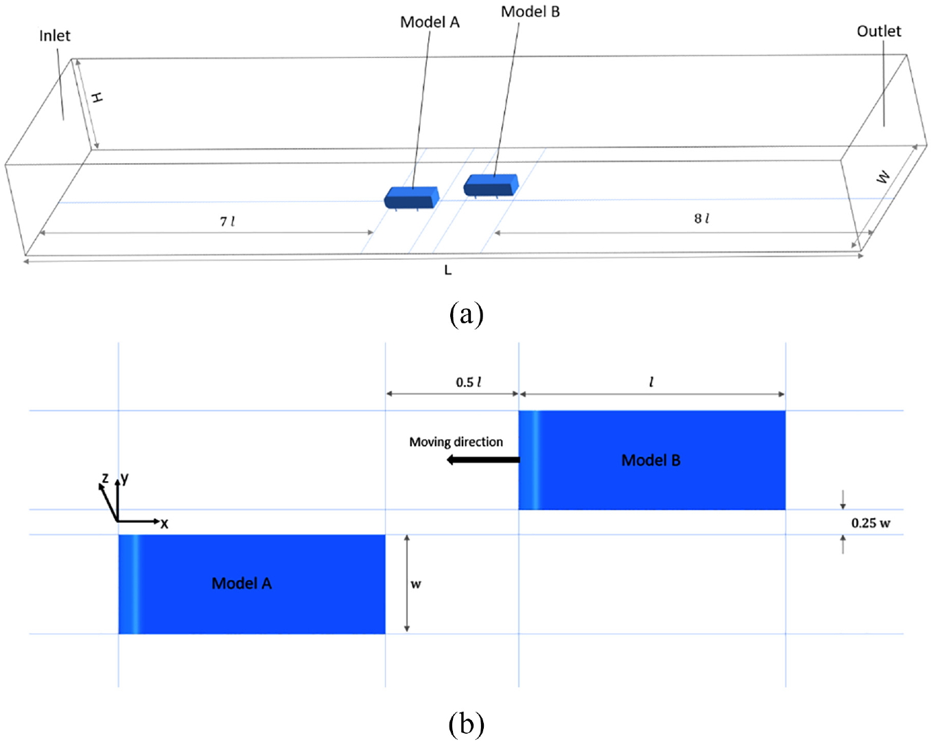
The origin of the Cartesian coordinates is at the middle of the two models on the floor, parallel to the front surface of the overtaken model (named Model A), as shown in Figure 2. Model A is fixed at the center line on the floor of the test section in wind tunnel and Model B is fixed at one of the seven streamwise locations $: - 1.5 l$ , $- 1.0 l$ , $- 0.5 l$ , $0.0 l$ , $0.5 l$ , $1.0 l$ , $1.5 l$ . This covers the $1.5 l$ lagging to $1.5 l$ leading positions for the overtaking process. For the cases of Model B being placed at the negative streamwise locations, the wake effects generated from Model B on Model A can be studied. In contrast, the blockade effect on Model A stemmed from Model B can be studied for the cases of Model B being placed at the positive streamwise locations. Figure 2 shows Model B lagging $1.5 l$ behind Model A. The experiment uses seven static tests.

Figure 2.

(a) Schematic diagram of the computational domain and (b) top view of the two models for the static test with Model B at x/l = 1.5.

The freestream velocity ( $u_{0}$ ), which was measured at a distant upstream position from Model A using a pitot tube, is 15 m/s, which corresponds to a Reynolds number (based on the model’s height) of $1.9 \times 10^{5}$ . A multichannel pressure system that is produced by Scanivalve Corp. and which uses seven miniature pressure scanning modules (Model ZOC 33/64 px²⁴) and a stand-alone data base (Model RAD 3200²⁵), was used to measure the surface pressure on Model A and Model B was not instrumented.

Each ZOC 33/64 px module contains 64 pressure sensors. The full-scale range of the pressure sensor is ±2490 Pa, with an accuracy of ±0.15%. The sampling rate for the pressure sensor is 250 Hz. There are 432 pressure taps distributed on all surfaces, except for the lower surface of Model A (see Figure 1(b)). All the pressure tapings are connected to the pressure scanner using flexible polyvinyl chloride tubes of 1.1 mm in diameter and 0.3 m length. A study by Irwin et al.²⁶ showed that phase distortions have a minor effect if tube is less than 0.3 m long. 32,768 pressure data readings were collected for each sensor to determine the mean pressure at the tapping position for the experiment.

Numerical method

Numerical simulation of the flow field during overtaking process used a CFD code, ANSYS Fluent,²⁷ in the study.

Governing equations and turbulence model

The present study uses the transient Reynolds-averaged Navier-Stokes equations for conservation of mass and momentum for a constant air density (ρ) and dynamic viscosity (μ) given as:

\frac{\partial u_{i}}{\partial x_{i}} = 0

(2)

\begin{matrix} ρ \frac{\partial u_{i}}{\partial t} + ρ \frac{\partial (u_{i} u_{j})}{\partial x_{j}} = - \frac{\partial p}{\partial x_{i}} + \frac{\partial}{\partial x_{i}} [μ (\frac{\partial u_{i}}{\partial x_{j}} + \frac{\partial u_{j}}{\partial x_{i}})] \\ + \frac{\partial}{\partial x_{i}} (- ρ \bar{u'_{i} u'_{j}}) \end{matrix}

(3)

where $u_{i}$ and $u'_{i}$ are the mean and fluctuating velocity of the ith component, respectively, and $p$ is the mean pressure. The Reynolds stress tensor ( $- ρ \bar{u'_{i} u'_{j}}$ ) is modeled using Boussineq’s analogy as:

- ρ \bar{u'_{i} u'_{j}} = μ_{t} (\frac{\partial u_{i}}{\partial x_{j}} + \frac{\partial u_{j}}{\partial x_{i}}) - \frac{2}{3} δ_{ij} k

(4)

where $μ_{t}$ is the eddy viscosity, which is determined using the turbulence model, $k$ is the turbulent kinetic energy and $δ_{ij}$ is the Kronecker delta function. For a steady state (i.e. static condition), the first term on the left-hand-side (LHS) of equation (3), which is a time derivative term, is set equal to zero and all the other terms are kept in simulation.

A previous study by the authors²⁰ showed that the SST $k - ω$ turbulence model is a reliable and economic two-equation RANS turbulence model for simulation of static-type overtaking so it is used for this study. The turbulent kinetic energy ( $k$ ) and its specific dissipation rate ( $ω$ ) are respectively solved using the corresponding transport equations. The specific dissipation rate for turbulent kinetic energy is defined as:

ω = \frac{1}{C_{μ}} \frac{ε}{k}

(5)

where ε is the dissipation rate for turbulent kinetic energy and $C_{μ}$ has a constant value of 0.09. The eddy viscosity in equation (4) is determined in terms of the solved k and $ω$ values. Details of the SST $k - ω$ model is given in a previous study of Menter.²⁸ One important characteristic of the SST $k - ω$ model is that it is applicable to the viscous sublayer of flow over a wall boundary. However, $x_{ip}^{+}$ must be smaller than 2 in the near-wall grid layout to ensure a correct prediction of the near-wall flow properties.²⁸

Boundary and initial conditions

The widths of both transverse (y) sides and the top of the vertical (z) side must be sufficiently large to ensure that the boundaries extend into the freestream regions to allow zero-gradient conditions to be applied. The bottom of the vertical side is placed on the floor of the wind tunnel so that the non-slip conditions are valid. In summary,

\frac{\partial ϕ}{\partial y} = 0 at y = \pm 5.51 w = \pm 1.5 m

(6)

\frac{\partial ϕ}{\partial z} = 0 at z = 7.44 h = 1.5 m

(7)

where $ϕ$ denotes a general dependent variable.

At z = 0 u = v = w = 0,

(8)

k = 0

(9)

ω = 0

(10)

Without the (measured) inlet and outlet conditions, the assumption cannot but be used. The assumed inlet conditions are as follows. The uniform distributions of the mean velocity components, the turbulent kinetic energy and its specific dissipation rate at the inlet are:

u_{in} = u_{0} and v_{in} = w_{in} = 0

(11)

k_{in} = 0.002 u_{0}^{2}

(12)

ω_{in} = 0.1 \frac{ρ}{μ} k_{in}

(13)

These inlet conditions apply to the upstream freestream region, so the flow is close to homogeneous turbulence. The zero-gradient conditions are imposed on all of the solved transport flow properties as the outlet conditions for flow approaching the fully-developed state in the downstream region from the lagging model, that is,

\frac{\partial ϕ}{\partial x} = 0

(14)

A previous study by the authors²⁰ showed that the inlet and outlet boundaries for a static test of the undertaking process are at least $7 l$ in front of the leading vehicle and $8 l$ behind the lagging vehicle. More detailed information and discussion on this issue is given in this previous study.²⁰

The initial condition is specified for the transient simulation of the overtaking process. At the beginning of the overtaking process for the transient simulation for a specific velocity, the overtaking vehicle (Model B) starts from $x / l = 2$ (positioned at the front surface of the model). A steady-state simulation of this static test using Models A and B at $x / l = 0$ and $2$ , respectively, is firstly performed and the result is the initial condition for the next transient simulation.

Computational domain and grid layout

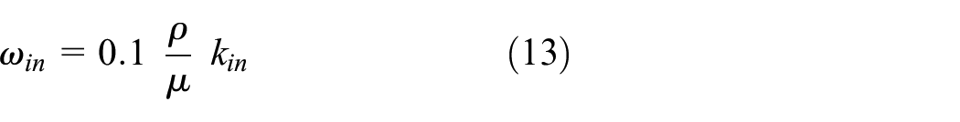
A hybrid mesh using hexahedral cells and tetrahedral cells is used for the computation, as shown in Figure 3. The tetrahedral mesh prism shape (Figure 3(a)) is used at the near-wall regions for models with curved head surfaces and allows the mesh to be generated more quickly. The hexahedral mesh type that is associated with the grid adaption technique is used at the periphery of the tetrahedral mesh (Figure 3(b)). A hybrid computational mesh is generated using ANSYS Meshing code.²⁹ The remaining space in the computational domain is constructed using hexahedral-type grids. The grid independent test was performed in a previous study by the authors²⁰ and its result is used for these computations and assures the near-wall grid condition of all $x_{ip}^{+}$ values less than 2, which satisfies the requirement for use of SST $k - ω$ turbulence model. The sliding mesh technique is used for mesh construction to allow Model B to move for the transient simulation of the overtaking process (Figure 4). The total number of mesh elements for the transient simulation, which requires the largest computational domain, is about 13.45 million.

Figure 3.

Mesh layout around the models: (a) side view and (b) top view for the static test with Model B at x/l = 1.0.

Figure 4.

Sliding meshes for Model B moving to position x/l = (a) 1.5, (b) 0.0, and (c) −1.5 during overtaking process.

The size of the computational domain varies with the simulation. Figure 2 shows the computational domain for the simulation of the static test using Model B placed lagging $1.5 l$ behind Model A, where the streamwise length L is $17.5 l$ . The shortest L ( $= 16 l$ ) occurs for the simulation of the static test with zero lagging distance (i.e. parallel) between the two models. Model B starts moving from position $x / l = 2$ and stops at $x / l = - 2$ for the transient simulations of the overtaking process so the sliding mesh technique and the required inlet and outlet distances give a streamwise length L = 22 $l$ for the computation.

Other numerical details

All transport differential equations are discretized using the QUICK scheme.³⁰ The SIMPLEC algorithm³¹ is used to deal with velocity-pressure coupling in the momentum equation, equation (3). The convergence criterion is that the residuals for all solved transport properties in the computational domain must reach their own asymptotic values, so these residual values cannot be further reduced with more iterations (or in every time step for a transient computation). For the transient computation, the time derivative term in equation (3) is discretized using the first-order implicit scheme. The time step ( $Δ t$ ) ranges between $8.56 \times 10^{- 5} s$ and $1.14 \times 10^{- 4} s$ , depending on the relative overtaking velocity for the simulation, to ensure that the CFL numbers are less than 0.99. The CFL number, Co, is calculated as

Co = u_{\max} \times \frac{Δ t}{Δ x_{\min}}

(15)

where $Δ x_{\min} = 1.73 \times 10^{- 3} m$ is the minimum grid size for the constructed grid mesh and $u_{\max}$ is the maximum velocity in the computation with the specified incoming freestream velocity and a relative overtaking velocity. To understand the effect of time step on the numerical performance, a small value of Co = 0.5 is purposely conducted for the overtaking case of r = 0.167; and the simulated results are compared to those predicted with Co = 0.99. The time steps are $9.78 \times 10^{- 5} s$ and $4.94 \times 10^{- 5} s$ corresponding to the two Co values of 0.99 and 0.5, respectively. The drag coefficient and side force coefficient predicted with these two cases of different time steps are displayed in Figure 5. Comparison results show negligible differences in between the simulation using these two time steps. It confirms that the set time step range is suitable for computations of the present overtaking simulation.

Figure 5.

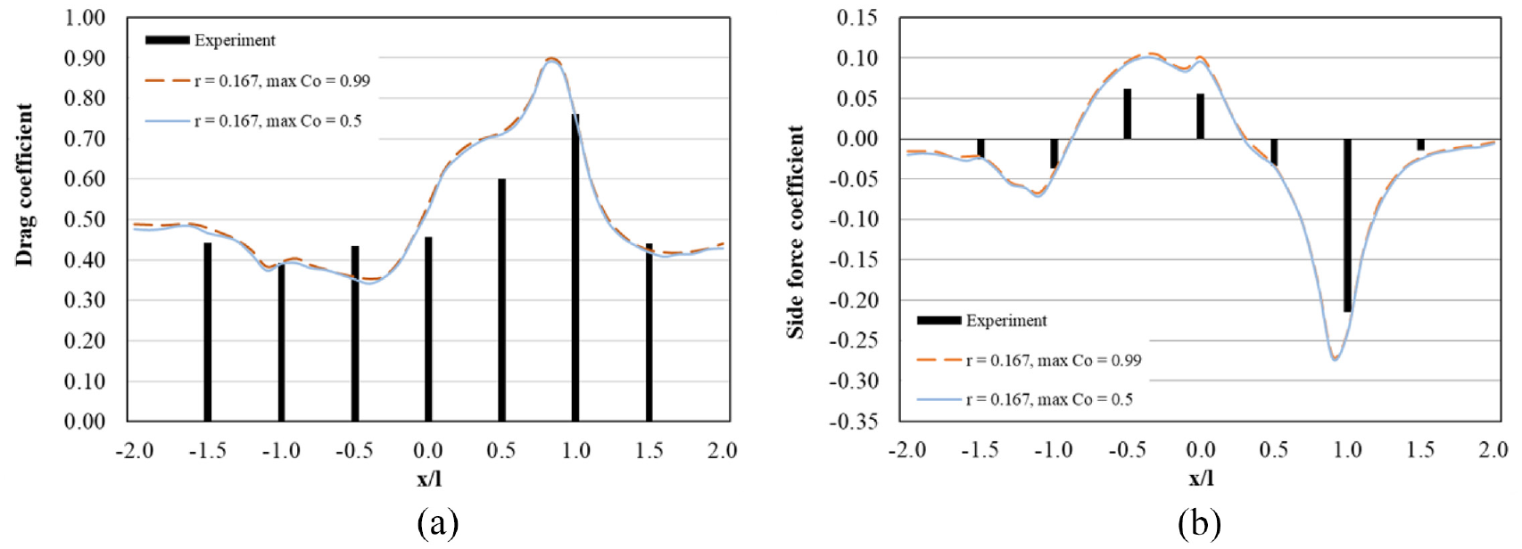
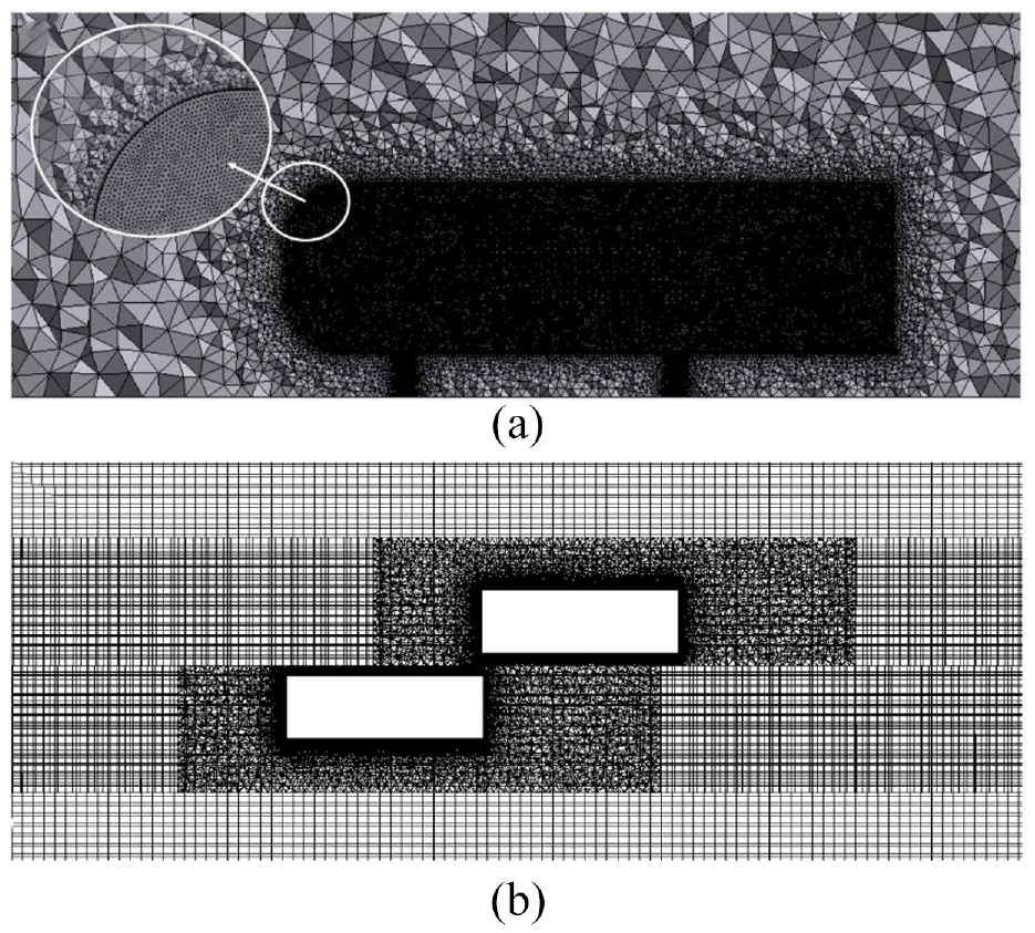
Comparison of the predicted: (a) drag coefficients and (b) side force coefficients on Model A in the overtaking simulation with r = 0.167 under the two CFL numbers.

Results and discussions

Static tests

Seven static tests were implemented experimentally and numerically. Model A was fixed at $x / l = 0$ and Model B was placed at $x / l = - 1.5$ , $- 1.0$ , $- 0.5$ , $0.0$ , $0.5$ , $1.0,$ and $1.5$ for each test. Model A is the overtaken vehicle when Model B is placed at positions $x / l > 0$ and is the overtaking vehicle when Model B is placed at positions $x / l < 0$ . A comparison of the measured and predicted distributions for the mean pressure coefficients ( $C_{p}$ ), defined below, along the centerlines of the right-hand side (RHS, the direction facing toward the Model B), the LHS, the frontal and rear surfaces on Model A are respectively shown in Figures 6 to 9.

C_{p} = \frac{p - p_{\infty}}{p_{d}}

(16)

where $p$ is the mean surface pressure, $p_{\infty}$ is the freestream static pressure, and $p_{d}$ is the freestream dynamic pressure ( $= \frac{1}{2} ρ u_{0}^{2}$ ). Each measured pressure coefficient is calculated using 32,768 instantaneous surface pressure data points and the error bars are attached at the point in the figures. The magnitude of a set of error bars is implicitly a steady extent of fluid motion so a larger magnitude for a set of error bars for the measured pressure coefficient demonstrates large-scale organized motion at that position in the flow. The distribution of the predicted turbulent kinetic energy, $k$ , on the middle plane ( $z / h = 0.607$ ) of the side surfaces for the seven static tests is shown in Figure 10 to interpret the interference of flow phenomena for the two models. The values for turbulent kinetic energy that are shown in Figure 11 are dimensionless (divided by $u_{0}^{2}$ ).

Figure 6.

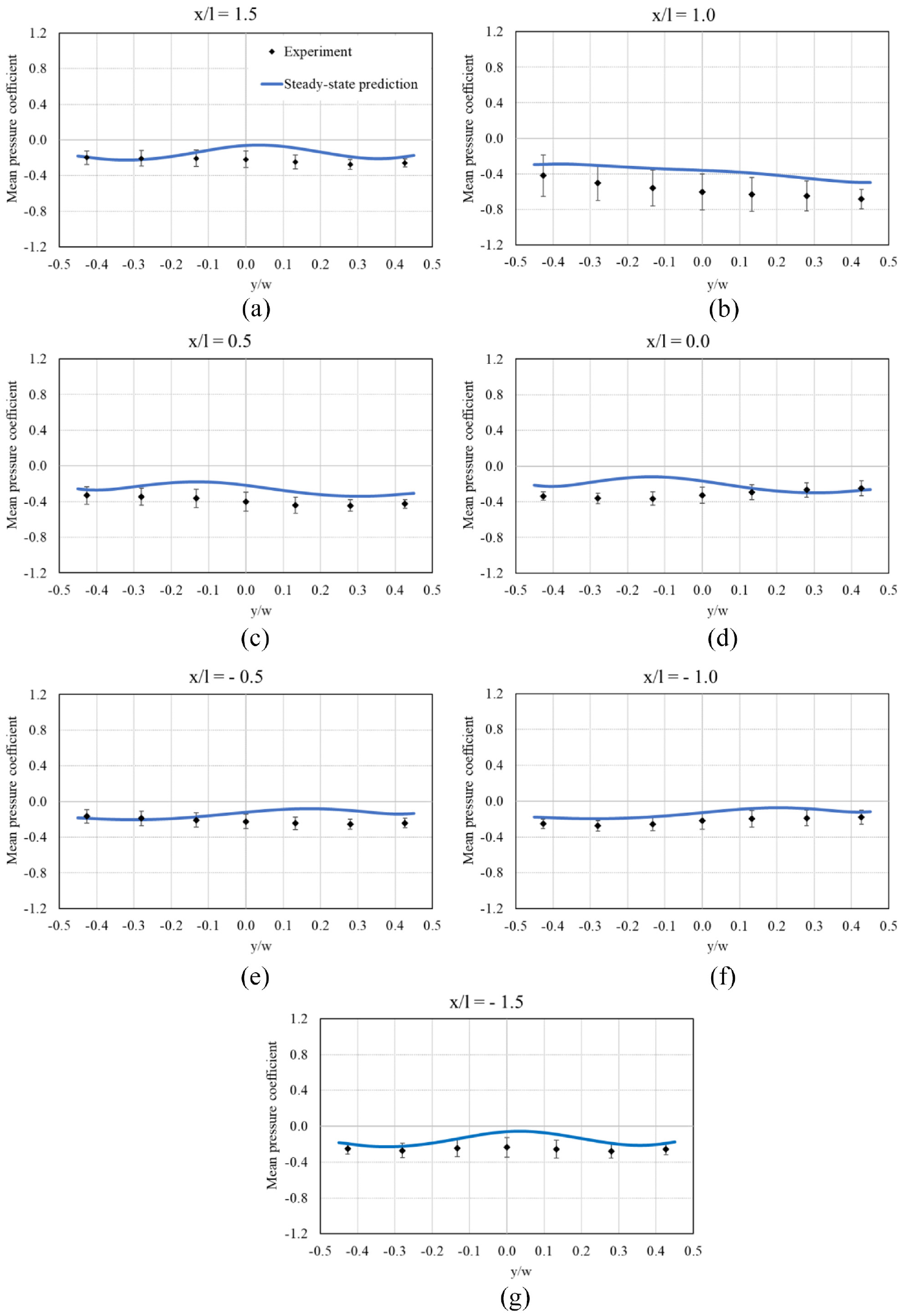
Distribution of mean pressure coefficient along the centerline of the right-hand side surface of Model A for Model B at x/l = (a) 1.5, (b) 1.0, (c) 0.5, (d) 0.0, (e) −0.5, (f) −1.0, and (g) −1.5.

Figure 7.

Distribution of mean pressure coefficient along the centerline of the left-hand side surface of Model A for Model B at x/l = (a) 1.5, (b) 1.0, (c) 0.5, (d) 0.0, (e) −0.5, (f) −1.0, and (g) −1.5.

Figure 8.

Distribution of mean pressure coefficient along the centerline of the frontal surface of Model A for Model B at x/l = (a) 1.5, (b) 1.0, (c) 0.5, (d) 0.0, (e) −0.5, (f) −1.0, and (g) −1.5.

Figure 9.

Distribution of mean pressure coefficient along the centerline of the back surface of Model A for Model B at x/l = (a) 1.5, (b) 1.0, (c) 0.5, (d) 0.0, (e) −0.5, (f) −1.0, and (g) −1.5.

Figure 10.

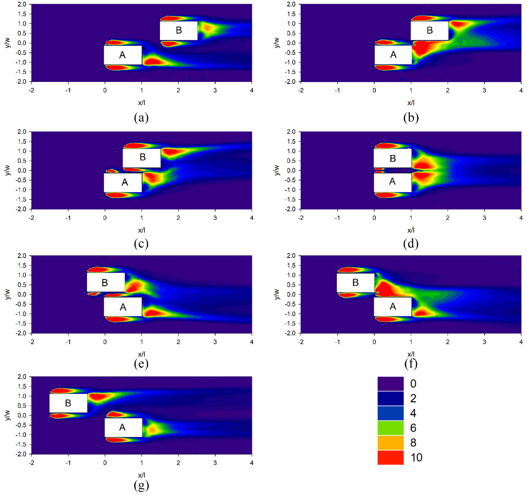
Distribution of the predicted turbulent kinetic energy on the middle planes (i.e. z/h = 0.607) for the two models for all seven static tests: (a) x/l = 1.5, (b) x/l = 1.0, (c) x/l = 0.5, (d) x/l = 0.0, (e) x/l = −0.5, (f) x/l = −1.0, and (g) x/l = −1.5.

Figure 11.

Comparison of the measured and predicted drag coefficients for Model A for all seven static tests.

When air passes over a bluff body, such as Model A in Figure 10(a), a boundary layer develops on each side surface. When this boundary layer grows, there is boundary layer separation and reattachment which are nonstationary flow phenomena, so there are significant error bars in the upstream region ( $x / l < 0.5$ in Figure 6(a)). After the reattachment position, the boundary layer develops again until air passes over the end of the side surface, so there are small error bars in the downstream regions ( $x / l > 0.5$ in Figure 6(a)).

However, the blockage effect of Model B, which is located at the RHS (with the transverse space of $0.25 w$ , see Figure 2(b)) behind Model A, inhibits the development of the boundary layer: more so on the RHS surface of Model A than on the LHS surface (compare Figure 6(a), (b), and (c) and Figure 7(a), (b), and (c)). The blockage effect that acts on the overtaken vehicle (Model A) increases as the lagging distance decreases, as shown by the comparison between Figure 6(a), (b), and (c). Nevertheless, when Model A overtakes (that is, when Model B is at $x / l < 0$ ), the wake that is formed behind Model B inhibits the development of a boundary layer on Model A: more so on the RHS surface than on the LHS surface (compare Figure 6(e), (f), and (g) and Figure 7(e), (f), and (g)). However, the wake effect becomes weaker as the leading distance increases, as shown in the comparison between Figure 6(e), (f), and (g).

The incoming air impinges on the frontal surface so the value of $C_{p}$ is positive along the centerline of Model A for all static tests. However, the blockage effect (Model B is at $x / l < 0$ ) or wake effect (Model B is at $x / l > 0$ ) on Model A is observed from the asymmetric extent (with respect to the y axis) of the transverse distributions for $C_{p}$ , particularly if the leading or lagging distance between Models A and B is short (see Figure 8). Wakes are formed behind the models. This flow phenomenon gives negative $C_{p}$ values (suction) along the centerline of the back surface of Model A, regardless of whether Model A is overtaken or overtaking. There is a more significant blockage or wake effect if the leading or lagging distance between Models A and B is shorter (see Figure 8).

The mean drag force coefficient is defined as:

C_{D} = \frac{\int_{A_{f}} C_{p, f} dA - \int_{A_{b}} C_{p, b} dA}{A_{c}}

(17)

where subscripts “ $f$ ” and “ $b$ ” respectively denote the front and back surfaces of Model A and $A_{c}$ is the cross-sectional area ( $= wh,$ also $= A_{b}$ ). The mean side force coefficient is defined as:

C_{Y} = \frac{\int_{A_{s}} (C_{p, l} - C_{p, r}) dA}{A_{s}}

(18)

where subscripts “ $l$ ” and “ $r$ ” respectively denote the LHS and RHS surfaces of Model A and $A_{s}$ is the area of the side surface. The mean drag coefficient is calculated using the measured mean pressure coefficients and equation (17) for the seven static tests and the results are shown in Figure 11 and Table 1. The measured mean side force coefficients for the seven static tests are calculated using equation (18) and the results are shown in Figure 12 and Table 2.

Table 1.

The measured and predicted drag coefficients that act on Model A for all seven static tests.

x/l	−1.5	−1.0	−0.5	0.0	0.5	1.0	1.5
Experiment	0.442	0.394	0.435	0.456	0.6	0.762	0.44
Steady-state	0.485	0.434	0.395	0.511	0.613	0.766	0.432
$Δ C_{D}$ (%)	9.73	10.15	−9.20	12.06	2.17	0.52	−1.82

Figure 12.

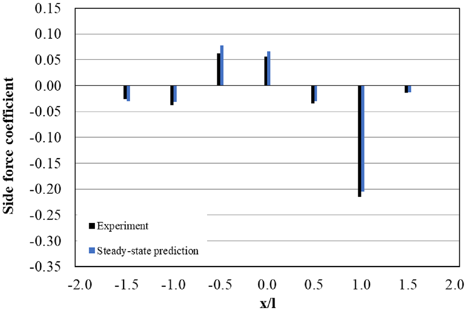
Comparison of the measured and predicted side force coefficients for Model A for all seven static tests.

Table 2.

The measured and predicted side force coefficients that act on Model A for all seven static tests.

x/l	−1.5	−1.0	−0.5	0.0	0.5	1.0	1.5
Experiment	−0.026	−0.037	0.062	0.056	−0.034	−0.215	−0.014
Steady-state	−0.03	−0.031	0.078	0.066	−0.03	−0.205	−0.013
$Δ C_{Y}$ (%)	15.38	−16.22	25.81	17.86	−11.76	−4.65	−7.14

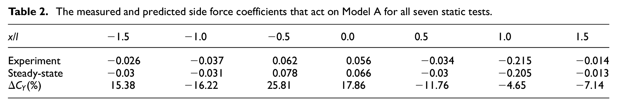
Figure 11 and Table 1 show that the blockage effect of Model B on the drag coefficient of Model A (overtaken role) varies significantly for the three static tests at $x / l > 0$ . It increases as the lagging distance for Model B of $x / l = 1.5$ decreases to $x / l = 1.0$ and then decreases until there is no blockage effect at $x / l = 0.0$ . The wake effect that is generated by Model B on the drag coefficient of Model A (overtaking role) varies less significantly for the three static tests at $x / l < 0$ , compared to the blockage effect for the static tests at’ $x / l > 0$ .

In terms of the variation of side force coefficient for the overtaking process, the results in Figure 12 and Table 2 show a similar trend to that for the drag coefficient (Figure 11) as the blockage effect from Model B on Model A (overtaken role) for the three static tests for which Model B is at $x / l > 0$ . If Model B is placed at two next upstream positions of $x / l = 0.0$ and $- 0.5$ , the side force that acts on Model A changes from repulsive force (negative side force) to suction force (positive side force). If Model B is at the more upstream positions of $x / l = - 1.0$ and $- 1.5$ , the side force that acts on Model A is again a repulsive force and the wake effect that is generated by Model B on the side force coefficient for Model A (overtaking role) varies less significantly than the drag coefficient (Figure 11).

Comparisons between the predicted and measured distributions for the mean pressure coefficient along the centerlines of two side surfaces are shown in Figures 6 and 7. There is satisfactory agreement, except in complicated subregions where the boundary layer separates and reattaches, which are located in the upstream part of the boundary layers on the surfaces, as shown in Figure 10. However, even in these complicated flow subregions, the predictions are acceptable. The predicted and measured distributions for the mean pressure coefficient along the centerlines of the frontal surface show good agreement, as shown in Figure 8. As mentioned previously, there is a wake with a coherent vortex structure behind Model A, regardless of where Model B is placed. Figure 9 shows that the mean pressure coefficients along the centerline of the back surface are predicted to be greater than the measured results.

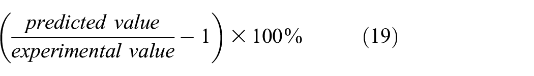
The mean drag coefficients and the mean side force coefficients are calculated using the predicted mean pressure coefficients for the seven static tests and the results are respectively shown in Figure 11/Table 1 and Figure 12/Table 2, for comparison with the measured results. The difference between the prediction and experiment for a specific mean force coefficient is calculated as:

(\frac{predicted value}{experimental value} - 1) \times 100 %

(19)

The difference between the predicted and measured drag coefficients and the side force coefficients at the seven static tests are calculated using equation (19) and the results are respectively shown in Tables 1 and 2. These differences are small for the blockage effect on Model A (overtaken) due to Model B (see Figure 10(a), (b), and (c)) and large for the wake effect on Model A (overtaking) due to Model B (see Figure 10(e), (f), and (g)). When the two models are parallel (see Figure 10(d)), the boundary layer that develops on the RHS surface and the wake structure behind the back surface of Model A is significantly inhibited by Model B, so the flow phenomena in the neighboring regions of Model A are very complicated. The isotropic assumption that is used to determine the eddy viscosity using the SST $k - ω$ turbulence model cannot be properly applied to this situation, so the results are significantly different to the experimental results.

The turbulent wake that is generated behind Model B in Figure 10(e), (f), and (g) features a coherent vortex structure, which is composed of large-scale organized motions and microscale fluctuating motions. The significant difference between the predicted and measured aerodynamic force coefficient for the wake effect can be attributed to use of the SST $k - ω$ model and is elaborated as follows.

RANS models use Reynolds decomposition, which is defined below, for statistical descriptions of a stationary turbulence.

U_{i} (\underline{x}, t) = u_{i} (\underline{x}) + {u^{'}}_{i} (\underline{x}, t)

(20)

where $U_{i}$ is the instantaneous velocity, $u_{i}$ is the time-independent mean velocity and $u'_{i}$ is the time-dependent fluctuation. For a large-scale organized motion in the wake flow, the time-dependent velocity comprises a coherent vortex and a randomly fluctuating part. The organized motion and the random fluctuation are uncorrelated. The instantaneous velocity data should be analyzed using the triple decomposition³² as:

U_{i} (\underline{x}, t) = u_{i} (\underline{x}) + {\tilde{u}}_{i} (\underline{x}, t) + {u ″}_{i} (\underline{x}, t)

(21)

where ${\tilde{u}}_{i}$ is the time-dependent part with zero mean due to the large-scale organized motion and $u {''}_{i}$ is the purely turbulent fluctuation part. The turbulence models such as the large eddy simulation (LES) and the detached eddy simulation (DES) use triple decomposition to formulate the model. Both models solve the first and second (time-dependent) terms on the RHS of equation (21) directly using the transient Navier-Stokes equations and the third (fluctuation) term is solved using a sub-grid turbulence model.

The numerical study for the turbulent flow field around an Ahmed body conducted by Guilmineau et al.²¹ employed the SST $k - ω$ , explicit algebraic stress, DES and an improved delayed eddy simulation (IDDES) models.³³ Through comparison with available experimental results, they showed better predicting capabilities of DES and IDDES models in the wake region than those of the RANS models including the SST $k - ω$ model. In particular, the IDDES model showed the best performances for the flow properties and phenomena among the four investigated turbulence models in their study. However, the mesh used for the simulation of one single Ahmed body with the IDDES model was 23.6 million elements, which has been already greatly larger than that (13.45 million elements) used for the present simulation of the overtaking process between two simplified Ahmed models with the SST $k - ω$ model. Florian et al.³⁴ recently simulated the turbulent flow over a single Ahmed body model using the LES model with a denser mesh of 40 million elements than that was used by Guilmineau et al.²¹ However, there were still observable differences in between the LES predictions and the experimental results in the study. It implies that a finer mesh, particularly in the near-wall subregions over the model’s walls, could be needed for LES to achieve better predictions. LES, DES or even the advanced DES-type turbulence model, thus, has potential to better simulate the wake effect that is generated by Model B on Model A than the RANS turbulence models, such as the SST $k - ω$ model for this study. However, using LES or DES-type turbulence models for simulation requires significantly more computational resources than using RANS models.

Transient simulations

The results of series of transient simulation involving different overtaking velocities are listed in Table 3. The distributions of the calculated drag and side force coefficients, using the predicted mean pressure coefficients for five values of $r$ are respectively shown in Figures 13 and 14 and compared with the experimental results for the static tests. For $r = 0$ in Figures 13 and 14, it is equivalent to the steady-state simulations.

Table 3.

The transient simulations for different overtaking velocities.

No.	$V (m / s)$	$V_{r} (m / s)$	$r$
1	15.000	5.000	0.333
2	15.000	2.500	0.167
3	15.000	1.500	0.100
4	15.000	0.750	0.050
5	15.000	0.500	0.033
6	15.000	0.315	0.021
7	15.000	0.210	0.014
8	15.000	0.105	0.007

Figure 13.

Comparison of drag coefficients for transient simulations using various overtaking velocities and for static tests.

Figure 14.

Comparison of side force coefficients for transient simulations using various overtaking velocities and for static tests.

In general, the variation trends in the predicted values of the transient simulation for $C_{D}$ and $C_{Y}$ match, to a certain extent, those for the static tests. The difference in $C_{D}$ and $C_{Y}$ between the predictions and the static-tests measurements at seven $x$ positions for various overtaking velocities for the static tests are calculated using equation (19). The corresponding maximum difference for each overtaking velocity is listed in Table 4. The maximum difference in $C_{D}$ and $C_{Y}$ increases as $r$ value increases, as shown in Table 4 or Figures 13 and 14. The maximum difference in $C_{D}$ and $C_{Y}$ for $r = 0.333$ (equivalent to $5 m / s$ overtaking velocity) between the transient simulation and the static experiment is 46.79% and 156.63%, respectively. The maximum difference in $C_{D}$ and ’ $C_{Y}$ between the steady-state ( $r = 0$ ) simulations and the static experiments, as shown in Tables 1 and 2, is 12.06% and 25.81%, respectively. Using these two values as the prediction uncertainties for the SST $k - ω$ model for the static test, the results in Table 4 show that the results for transient simulations for which $r \leq 0.021$ are within the prediction uncertainties. If $r \leq 0.021,$ this is equivalent to fitting using the steady state approach. The experimental study of the Noger et al.¹¹ showed that there is a small transient effect on the aerodynamic force for $r < 0.25$ for the overtaken vehicle and for ’ $r < 0.2$ for the overtaking vehicle. Corin et al.¹⁵ conducted steady-state and transient two-dimensional simulations of the overtaking process and concluded that the steady-state approach is not accurate for $r > 0.2$ . However, the predicted transient results for $r = 0.167$ that are shown in Figures 13 and 14 still exhibit significant differences to those for the static tests. These differences are small for $r \leq 0.1$ , so the steady-state approach can be acceptably used as the quasi-steady condition for dynamic cases for which $r \leq 0.1$ .

Table 4.

Maximum deviation in the drag and side forces coefficients that act on Model A between for a transient simulation for different r values and obtained for experimental static tests (i.e. r = 0).

r	0.333	0.167	0.100	0.050	0.033	0.021	0.014	0.007
$\max Δ C_{D}$ (%)	46.79	19.44	14.26	12.42	12.08	11.83	11.36	10.72
$\max Δ C_{Y}$ (%)	156.63	80.93	46.61	32.70	28.80	25.55	19.63	18.38

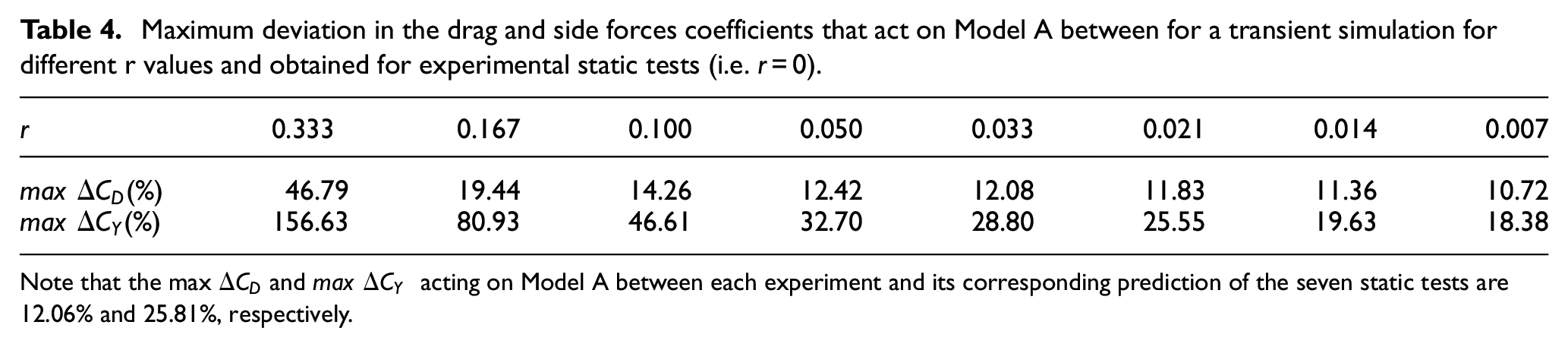
Note that the max $Δ C_{D}$ and $\max Δ C_{Y}$ acting on Model A between each experiment and its corresponding prediction of the seven static tests are 12.06% and 25.81%, respectively.

The distributions for turbulent kinetic energy on the middle planes of the two models for the steady-state simulations are mirror images of each other (Figure 10), including those in Figure 10(a) and (g) (for $x / l = 1.5$ and $- 1.5$ , respectively), Figure 10(b) and (f) (for $x / l = 1.0$ and $- 1.0$ , respectively) and Figure 10(c) and (e) (for $x / l = 0.5$ and $- 0.5$ , respectively). The distributions of turbulent kinetic energy on the middle plane of the two models are plotted in Figure 15 for a transient simulation for which $r = 0.333$ . There are none of the mirror image pairs that are seen in Figure 10 for the transient simulations. This shows another difference in the prediction between the steady-state and transient simulations for the overtaking process.

Figure 15.

Distribution of the predicted turbulent kinetic energy on the middle planes (i.e. z/h = 0.607) for the two models at seven different streamwise positions for a transient simulation for which r = 0.333: (a) x/l = 1.5, (b) x/l = 1.0, (c) x/l = 0.5, (d) x/l = 0.0, (e) x/l = −0.5, (f) x/l = −1.0, and (g) x/l = −1.5.

Conclusions

A set of static tests involving the overtaken and overtaking entities is numerically and experimentally studied using two simplified Ahmed body models. Numerical simulations use the SST $k - ω$ turbulence model, which predicts near-wall flow behavior well if there is an appropriate near-wall grid mesh. However, there are notable differences in the drag and side force coefficients for the predicted and experimental results of the wake effect on the overtaking model as well as under a situation when the two models are parallel for the static tests. This difference is attributed to the inadequacy of the SST $k - ω$ model, which is a two-eq22 RANS turbulence model and makes an isotropic eddy viscosity assumption. A more advanced turbulence model that can simulate large-eddy organized motion in the turbulent flow and which uses an anisotropic eddy viscosity formulation in the near-wall flow subregion, such as IDDES model, would increase the prediction accuracy of the aerodynamic forces during the overtaking process.

A comparison of the drag and side force coefficients for the transient simulations using various relative velocity ratio ( $r$ ) and those for the experimental static tests shows that the difference is 46.79% and 156.63%, respectively, for $r = 0.333$ . The quasi-steady simulation can be applied for the dynamic two-vehicle overtaking process for which $r \leq 0.1$ .

Footnotes

Appendix

Handling Editor: Chenhui Liang

Declaration of conflicting interests

The author(s) declared no potential conflicts of interest with respect to the research, authorship, and/or publication of this article.

Funding

The author(s) disclosed receipt of the following financial support for the research, authorship, and/or publication of this article: The authors acknowledge the funding support of the Ministry of Science and Technology of Republic of China under Grant Contract MOST 106-2218-E-0069–18–MY 1 and 2.

ORCID iD

Keh-Chin Chang

References

Heffley

RK.

Aerodynamics of passenger vehicles in close proximity to trucks and buses. SAE Trans 1973; 82: 901–914.

Howell

Garry

Holt

The aerodynamics of a small car overtaking a truck. SAE Int J Passeng Cars - Mech Syst 2014; 7: 626–638.

Howell

The influence of the proximity of a large vehicle on the aerodynamic characteristics of a typical car. In: Stephens

(ed.) Advances in road vehicle aerodynamics. Bedford, UK: BHRA Fluid Engineering, pp.207–221.

Yoshida

Muto

Imaizumi

Transient aerodynamic forces and moments on models of vehicles passing through cross-wind. SAE paper 770391, 1977,

Abdel Azim

. An experimental study of the aerodynamic interference between road vehicles. SAE paper 940422, 1994.

Noger

Grevenynghe

EV.

On the transient aerodynamic forces induced on heavy and light vehicles in overtaking processes. Int J Aerodyn 2011; 1: 373–383.

Minato

Ryu

Kobayashi

Aerodynamics of road vehicles in tunnels - flow visualization using the laser light sheet method and its digital image processing. SAE paper 910314, 1991

Abdel Azim

Abdel Gawad

. A flow visualization study of the aerodynamic interference between passenger cars. SAE paper 2000-01-0355, 2000.

Kremheller

Aerodynamic interaction effects and surface pressure distribution during on-road driving events. SAE paper 2015-01-1527, 2015.

10.

Yamamoto

Yanagimoto

Fukuda

, et al. Aerodynamic influence of a passing vehicle on the stability of the other vehicles. JSAE Rev 1997; 18: 39–44.

11.

Noger

Regarding

Széchényi

Investigation of the transient aerodynamic phenomena associated with passing maneuvers. J Fluids Struct 2005; 21: 231–241.

12.

Clarke

Filippone

Unsteady computational analysis of vehicle passing. J Fluids Eng 2006; 129: 359–367.

13.

Uystepruyst

Krajnovic

Numerical simulation of the transient aerodynamic phenomena induced by passing maneuvers. J Wind Eng Ind Aerod 2013; 114: 62–71.

14.

Shao

Yao

Zhang

, et al. A research into the flow and vortex structures around vehicles during overtaking maneuver with lift force included. Adv Mech Eng 2017: 9; 1–16.

15.

Corin

Dominy

RG.

A CFD investigation into the transient aerodynamic forces on overtaking road vehicle models. J Wind Eng Ind Aerod 2008; 96: 1390–1412

16.

Liu

Sun

Chi

, et al. Transient aerodynamic characteristics of vans overtaking in crosswinds. J Wind Eng Ind Aerod 2017; 170: 46–55.

17.

Duell

George

AR.

Experimental study of a ground vehicle body unsteady near wake. SAE paper 1999-01-0812, 1999.

18.

Sims-Williams

Dominy

Howell

JP.

An Investigation into large scale unsteady structures in the wake of real and idealized hatchback car models. SAE paper 2001-01-1041, 2001.

19.

Rao

Minelli

Basara

, et al. On the two flow states in the wake of a hatchback Ahmed body. J Wind Eng Ind Aerod 2018; 173: 262–278.

20.

Do Van

Chang

Chou

. Aspects on numerical simulation of overtaking process between two vehicles. J Aeronaut Astronaut Aviat Ser 2022; 54: 161–178.

21.

Guilmineau

Deng

Leroyer

, et al. Assessment of hybrid RANS-LES formulations for flow simulation around Ahmed body. Comput Fluids 2018; 176: 302–319.

22.

Sun

Karadimitriou

, et al. Aerodynamic interference between two road vehicle models during overtaking. J Energy Eng 2019; 145: 04019002.

23.

Ahmed

Ramm

Faltin

Some salient features of time averaged ground vehicle wake. SAE paper 840300, 1984.

24.

ZOC 33 Service Manual Sect. 2, Scanivalve Corp. 2016.

25.

ERAD 4000 Service Manual Sect. 2, Scanivalve Corp. 2019.

26.

Irwin

Cooper

Girard

Correction of distortion effects caused by tubing systems in measurements of fluctuating pressures. J Wind Eng Ind Aerod 1979; 5: 93–107.

27.

ANSYS Fluent Version 18.00. User’s Guide, ANSYS Inc., 2018.

28.

Menter

Two-equation eddy-viscosity turbulence models for engineering applications. AIAA J 1994; 32: 1598–1605.

29.

ANSYS Meshing Version 18.00. User’s Guide, ANSYS Inc. 2018.

30.

Leonard

BP.

A stable and accurate convective modeling procedure based on quadratic upstream interpolation. Comput Method Appl Mech Eng 1979; 19: 59–98.

31.

Van Doormaal

Raithby

. Enhancement of the SIMPLE method for predicting incompressible fluid flows. Numer Heat Transf 1984; 7: 147–163.

32.

Hussain

AKMF

Reynolds

. The mechanics of an organized wave in turbulent shear flow. J Fluid Mech 1970; 41: 241–258.

33.

Shur

Spalart

Strelets

, et al. A hybrid RANS-LES approach with delayed-DES and wall-modelled LES capabilities. Int J Heat Fluid Flow 2018; 29: 1638–1649.

34.

Florian

Andreas

Alexey

, et al. An overview of hybrid RANS–LES models developed for industrial CFD. Appl Sci 2021; 11: 2459.

Numerical and experimental study of two-vehicle overtaking process

Abstract

Keywords

Introduction

Experimental method

Numerical method

Governing equations and turbulence model

Boundary and initial conditions

Computational domain and grid layout

Other numerical details

Results and discussions

Static tests

Transient simulations

Conclusions

Footnotes

Appendix

Declaration of conflicting interests

Funding

ORCID iD

References