Sage Journals: Discover world-class research

Abstract

Aiming at the problem that the current isotropic virtual material-based modeling method for dynamic modeling of sliding joints can hardly reflect the difference between normal and tangential mechanical properties, which restricts the modeling quality, a transversely isotropic material model is introduced to comprehensively describe the mechanical properties of sliding joints. Firstly, a dynamic model based on transversely isotropic virtual material and Deep Neural Network (DNN) is constructed to reflect the relationship between the dynamic parameters of transversely isotropic virtual material $(E_{τ}, E_{n}, μ_{τ}, μ_{n}, G_{n}, ρ)$ and the natural frequencies. Then, using the cuckoo search algorithm, the transversely isotropic virtual material parameters are determined. Subsequently, as an application case, the flat and V-guide joints of the M7120D/H surface grinder are employed to validate the proposed modeling method. Finally, compared to the experimental modal test results, the error of natural frequencies is less than 1%, which achieves high accuracy. Additionally, the quantitative comparison based on the same application case shows that the proposed modeling method is superior to isotropic virtual material and spring damping method.

Keywords

Sliding joint transversely isotropic virtual material deep neural network dynamic modeling machine tool

Introduction

Sliding guide structures of machine tools are usually accompanied by sliding joints, which play a crucial role in the dynamic performance of the whole machine tool.^1–3 Therefore, the accurate dynamic modeling of sliding joints is essential to achieve precise predictions of the static and dynamic characteristics of machine tools.^4,5

Establishing an equivalent model is the prerequisite for the dynamic modeling of sliding joints. For the equivalent modeling of joints, virtual material is presently widely adopted.^6–9 It regards the joint as a virtual material layer of equal cross-section and is rigidly connected to two components on both sides.¹⁰ In the process of equivalent modeling with the virtual material method, the joint is normally simplified as an isotropic virtual material. Shi et al.¹¹ verified the feasibility of the equivalent virtual material model of fixed joints by taking two stepped steel plates connected by four bolts as an example. Based on the principle of equal strain energy, Ye et al.¹² derived the elastic modulus, Poisson’s ratio, and other parameters of the virtual material of the bolted fixed joints. Cui et al.¹³ proposed the response surface method (RSM) to identify the isotropic virtual material parameters of the bolted joint. Du et al.¹⁴ determined the parameters of the material layer of the fixed joint of the tie-bolt rotor based on 3D fractal contact theory and elastic-plastic contact theory.

The above literature demonstrates the validity of the isotropic virtual material method. However, as a particular form of virtual material, isotropic virtual material is only exact when the mechanical properties of joints are similar in all directions, including the normal direction, which is a relatively restrictive condition. In engineering practice, the mechanical properties of joints change significantly in the normal direction due to the mechanism of subsurface layer formation and evolution in the metalworking process, leading to the fact that ideal joints with uniform mechanical properties rarely exist.¹⁵ As a result, the isotropic virtual material cannot comprehensively reflect the mechanical properties of joints in different directions, which causes certain limitations in the equivalent modeling accuracy. Consequently, some scholars attempted to improve the equivalent modeling accuracy with transversely isotropic or nonlinear virtual materials.^16–19 Sun et al.¹⁸ proposed a parametric representation model of the bolted joint based on gradient virtual material to accurately characterize the asymmetric surface pressure distribution, which showed it was an efficient method for characterizing the stiffness distribution of bolted joints. Zhao et al.¹⁹ extracted the transversely isotropic virtual material parameters, reflecting the coupling between the normal and tangential stiffness of the fixed joint in the form of virtual material properties, and obtained extremely high consistency in the experimental and analytical results, which proved the correctness and rationality of this equivalent model. By introducing a calculation method of elastic modulus of composite materials, Zha et al.²⁰ proposed an improved transversely isotropic virtual materials model, which achieved significantly higher equivalent modeling accuracy than the conventional isotropic virtual material and spring damping method for bolted joints. Compared with the isotropic virtual material method, the transversely isotropic virtual material method emphasizes the difference between normal and tangential mechanical properties, which is more in line with the machined metal surfaces in engineering.^21,22 Therefore, it can be foreseen that it is more appropriate to equate sliding joints to transversely isotropic virtual material. Although transversely isotropic virtual material is currently primarily applied in the equivalent modeling of fixed joints²³ and seldom applied in sliding joints, they are all planar contacts with certain similarities. It is assumed that the equivalent modeling accuracy of sliding joints can be further improved by transversely isotropic virtual material.

For the dynamic modeling of sliding joints, some scholars have set up the relationship among the dynamic parameters of joints by establishing an analytical model.^24–26 Based on the principle of the Single-Degree-of-Freedom System, Guo et al.²⁴ derived an analytical model for identifying dynamic stiffness and conducted experiments on a self-developed test sliding platform to obtain the law of sliding speed, interfacial pressure medium, and other factors on the effect of stiffness. Wang et al.²⁵ analyzed the structural characteristics of sliding joints of a double-flat sliding guide and derived the analytical dynamic equation based on the Reynolds equation considering boundary lubrication and fractal theory. Based on the discrete Iwan modeling idea, Zong et al.²⁶ used the Jenkins elements to simulate the tangential stick-slip properties of sliding joints considering features of fractal surfaces under normal loading conditions. However, due to the complicated factors affecting the sliding joints, these analytical models usually focus on only certain features. They are inevitably simplified, resulting in certain constraints on modeling accuracy. As a modern numerical analysis computational method, FEA is widely used in dynamic characteristic analysis and structural optimization design.^27–29 Based on the stiffness matrix of the six-node contact unit, Wang et al.²⁷ established the FEA model considering sliding joints of machine tool guideways through the GiD Pre- and Post-Processing System. The comparison of the experimental results of the machine stiffness with the calculated results confirmed the validity of the method. However, due to the difficulty in knowing the equivalent parameters in advance, there is a problem of assigning initial values when modeling and a lack of possibility to implement reverse identification and correction of the dynamic parameters, which makes it difficult to apply such models forward. In response to the above problems, others have used shallow neural networks as an alternative to FEA to build dynamic models that can be directly embedded in optimization algorithms.^30,31 Zhu et al.³⁰ adopted GA-BP neural network as the dynamic model for identifying the stiffness and the damping of sliding joints. The parameter identification error was <5%. Pan et al.³¹ employed Elman neural network to develop the dynamic model for predicting the nonlinear friction behavior of a hydraulic cylinder system. The above neural networks allow the parameters to be identified by inverse optimization and, as a theoretical alternative, they are trained based on a large amount of data, eliminating the one-sidedness of the analytical model. Nevertheless, the shallow network is limited by its computational units, which still cannot map complex data.³² The dynamic characteristics of sliding joints are usually affected by many factors.^33,34 With different positions, types of guideways, and the increase in the number of sliding joints, the dynamic parameters involved will be multiplied, which makes the dynamic model characterized by multi-input and output and a high degree of complexity.^35,36 Currently, the modeling method based on the shallow network can hardly meet the above characteristics, thus still restricting the modeling accuracy.

DNN has powerful feature representation and data fitting capabilities and outperforms shallow networks for most applications in which high-dimensional data needs to be processed.^37,38 Zhu et al.³⁹ used DNN to establish the equivalent dynamic model of the critical joints of the ball screw feeding system, which greatly improved the identification accuracy of the dynamic characteristic parameters. Zhang et al.⁴⁰ used DNN to obtain the dynamic model of sliding joints, with stiffness and damping in X, Y, and Z directions as input and natural frequencies as output and achieved a smaller identification error of <3% than previous studies. From the above literature, DNN is excellent at handling complicated data problems, which makes it suitable for constructing the dynamic model with high-dimensional parameters. Consequently, if DNN is applied to establish the dynamic model of sliding joints, the modeling accuracy will be further improved.

Therefore, given the problem that the isotropic virtual material method is challenging to reflect the difference between the normal and tangential mechanical properties of joints, this study takes the M7120D/H surface grinder as an example. Firstly, its sliding joints are equated based on transversely isotropic virtual material, and then the dynamic model is established by DNN, which reflects the relationship between the dynamic parameters of the virtual material and the natural frequencies. Subsequently, based on the experimental modal test results, the optimization objective function is constructed. Finally, the parameters of transversely isotropic virtual material are obtained by the cuckoo search algorithm, which achieves extremely high identification accuracy.

The rest of the paper is organized as follows. The “Basic principle” section introduces the basic principle of the proposed method. In the “Application case study” section, the method proposed is verified based on sliding joints of the M7120D/H horizontal axis surface grinder. In the “Results and discussion” section, the method in this study is compared with the spring damping method and isotropic virtual material method. In the “Conclusion” section, the methodology of this paper is summarized and evaluated, and the potential future work is discussed.

Basic principle

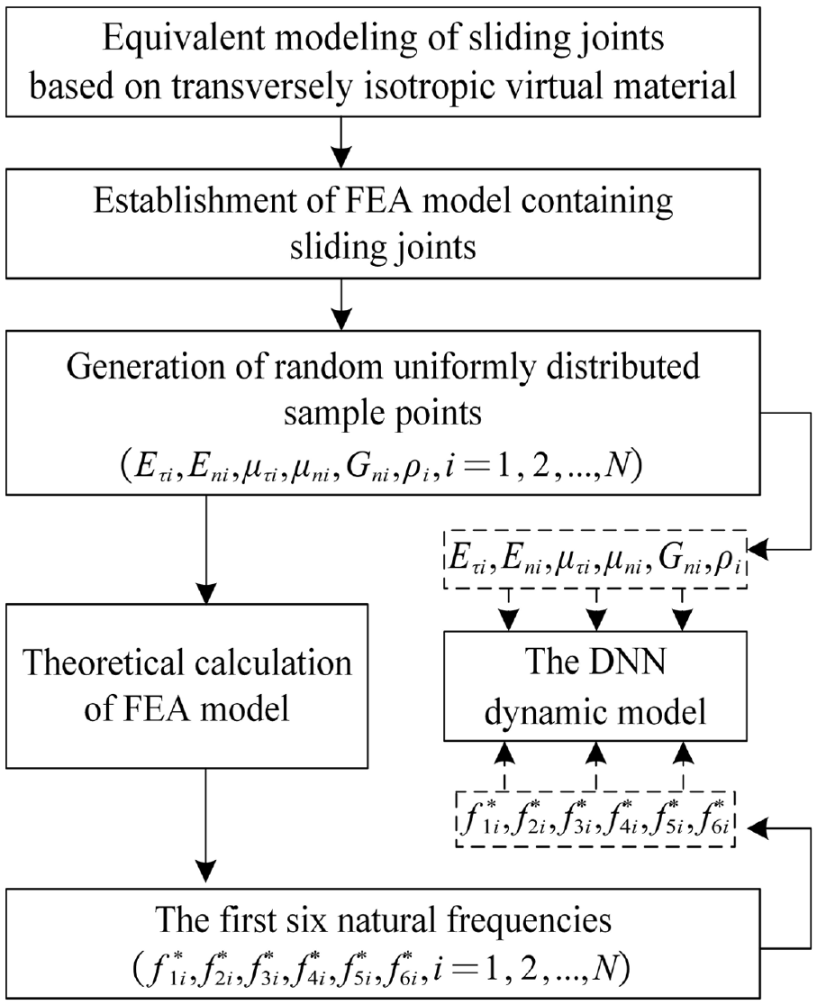
The principle of the dynamic modeling method proposed in this study is shown in Figure 1, which consists of four parts: the equivalent modeling, the establishment of the DNN dynamic model, the experimental modal test and the identification of dynamic parameters.

Figure 1.

Overall flow chart of dynamic modeling based on transversely isotropic virtual material and DNN.

Equivalent modeling of sliding joints

Firstly, the FEA model considering sliding joints is constructed for the establishment of the equivalent model, and then the virtual material parameters which can characterize dynamic properties are substituted into the constructed FEA model for the theoretical analysis, after which the natural frequencies are acquired. Through the parametric calculation of different transversely isotropic virtual material parameters within a certain range, a data set for DNN training is generated.

Establishment of the DNN dynamic model

Through the large amount of data generated by FEA software, the DNN is thoroughly trained and tested, which is essential for building highly accurate models that reflect the relationships among dynamic characteristic parameters.

Experimental modal test

During the experimental modal test, multiple testing points are set on mechanical parts on both sides of sliding joints, and a suitable position is selected for placing accelerometer sensors. The vibration signal generated by hammering is collected and analyzed in the analysis system to obtain the natural frequencies.

Identification of dynamic parameters

The error between the predicted values of the DNN dynamic model and the experimental values is constructed as an objective function. Through the cuckoo search algorithm, an optimal identification model is established for the reverse identification of the material parameters.

Equivalent modeling of sliding joints based on transversely isotropic virtual material

As shown in Figure 2, the microstructure of the sliding joint is a layered structure, and each micro-layer has a different mechanical property.^21,22 The mechanical properties of the sliding joint change dramatically in its normal direction, while the surfaces of the sliding joint are microscopically multiscale and disordered.²³ Therefore, along the tangential direction, the mechanical properties of the joint are the same, and synchronously, there is a significant difference between its normal and tangential mechanical properties. According to this characteristic, the study proposes an equivalent modeling method for sliding joints based on transversely isotropic virtual material to simulate the dynamic characteristics of sliding joints more accurately.

Figure 2.

Sliding joint of machine tool and its transversely isotropic characteristic.

The equivalent modeling principle is shown in Figure 3, which regards the sliding joint as a transversely isotropic virtual material layer with an equal cross-section and a specific thickness, rigidly connected to the skid platform and guideway.

Figure 3.

Schematic diagram of the sliding joint equivalent model.

The dynamic equation for the virtual material method⁴¹ is expressed in equation (1):

[(\begin{matrix} M_{1} \\ M_{2} \end{matrix}) + M_{v}] (\begin{matrix} {\overset{\cdot\cdot}{x}}_{1} \\ {\overset{\cdot\cdot}{x}}_{2} \end{matrix}) + [(\begin{matrix} K_{1} \\ K_{2} \end{matrix}) + K_{v}] (\begin{matrix} x_{1} \\ x_{2} \end{matrix}) = (\begin{matrix} F_{1} \\ F_{2} \end{matrix})

(1)

where, 1 represents the skid platform and 2 represents the guideway. M is the mass matrix. K is the stiffness matrix and V is the virtual material layer. F represents the external force on the structure.

When using the FEA method, the element stiffness matrix of virtual material can be obtained from the following equations (2) and (3):

{[K_{V}]}^{e} = \int_{Ω^{e}} B_{V}^{T} D B_{V} d_{Ω}

(2)

B_{V} = \partial \cdot N_{V} .

(3)

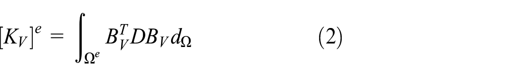
where, D represents the elastic matrix, and B represents the strain matrix. N represents the shape function.

This study uses the flexibility matrix S (equation (4)) as the input. S is the reciprocal matrix of D, that is, $D = S^{- 1}$ , and the other variables can be calculated by FEA software.

The flexibility matrix S based on transversely isotropic virtual material can be expressed as follows:

S = (\begin{matrix} 1 / E_{τ} & - μ_{τ} / E_{τ} & - μ_{n} / E_{n} \\ - μ_{τ} / E_{τ} & 1 / E_{τ} & - μ_{n} / E_{n} \\ - μ_{n} / E_{n} & - μ_{n} / E_{n} & 1 / E_{n} \\ 1 / G_{τ} \\ 1 / G_{n} \\ 1 / G_{n} \end{matrix})

(4)

Accordingly, the parameters of the virtual material layer are normal elastic modulus $E_{n}$ , normal Poisson’s ratio $μ_{n}$ , normal shear modulus $G_{n}$ , tangential elastic modulus $E_{τ}$ , tangential Poisson’s ratio $μ_{τ}$ , tangential shear modulus $G_{τ}$ , and the material’s inherent parameter density $ρ$ . According to the properties of transversely isotropic virtual material, the tangential shear modulus satisfies $G_{τ} = E_{τ} / 2 (1 + μ_{τ})$ . Therefore, a single sliding joint contains six independent parameters.

When using FEA software to establish the equivalent model of sliding joints, the parameters of the above virtual material can be set by the Linear Elastic Material function in the Solid Mechanics module of COMSOL Multiphysics. In this way, the strain-stress constitutive relation of virtual material is obtained to simulate the dynamic characteristics of the joint.

The theoretical data set for DNN model training is then generated with COMSOL parametric calculation, containing N sets of sample points $(E_{ni}, μ_{ni}, G_{ni}, E_{τ i}, μ_{τ i}, ρ_{i}, i = 1, 2, . . ., N)$ and N sets of results $(f_{1 i}^{*}, f_{2 i}^{*}, f_{3 i}^{*}, f_{4 i}^{*}, f_{5 i}^{*}, f_{6 i}^{*}, i = 1, 2, . . ., N)$ corresponding to the samples.

Establishment of the DNN dynamic model

After the establishment of the equivalent model, many parameter sample points are generated within a certain parameter range, and the first six natural frequencies corresponding to the sample points are calculated in FEA software to train the DNN dynamic model. Concretely, the DNN dynamic model is established according to the basic principle shown in Figure 4. Its main processes include:

(1) The sample points of the virtual material parameters are generated by random uniform distribution for the uniformity and independence of the data distribution. The N sample points generated are elastic modulus $(E_{τ i}, E_{ni}, i = 1, 2, . . ., N)$ , Poisson’s ratio $(μ_{τ i}, μ_{ni}, i = 1, 2, . . ., N)$ , shear modulus $(G_{ni}, i = 1, 2, . . ., N)$ , and density $(ρ_{i}, i = 1, 2, . . ., N)$ .

(2) In the FEA model containing sliding joints, the generated samples are parametric calculated to obtain the result sequences $(f_{1 i}^{*}, f_{2 i}^{*}, f_{3 i}^{*}, f_{4 i}^{*}, f_{5 i}^{*}, f_{6 i}^{*}, i = 1, 2, . . ., N)$ corresponding to each of these N samples, and the samples are then combined with the result sequences to generate the data set.

(3) The DNN model is designed with the virtual material parameters as the input and the sliding joint’s first six natural frequencies as the output. The data set generated in step 2 is split into a training set and a test set to train the DNN dynamic model of sliding joints.

Figure 4.

Modeling and training of DNN dynamic model.

The DNN consists of a topological structure, activation function, loss function, and training algorithm.³⁸ It has multiple hidden layers to represent the mapping relationship of complex and high-dimensional data, and its structure is shown in Figure 5.

Figure 5.

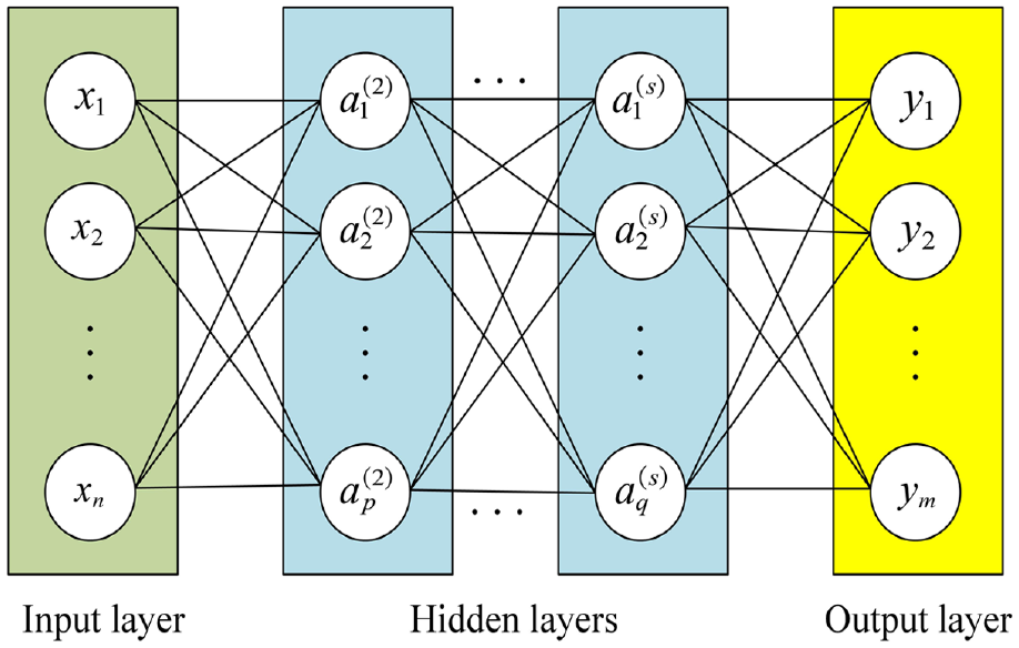
The structure of DNN.

However, deep hidden layers not only increase the computational cost but also the feedback information of the error will decay, which makes it difficult to update the correction information and makes the training challenging to converge. Meanwhile, too few or too many neurons in hidden layers will lead to an incomplete fit. Therefore, when designing the DNN model, it is necessary to design a reasonable topology. The number of neurons in each hidden layer can be determined by equation (5):

N_{h} = ⌈ \sqrt{N_{h - 1} + N_{h + 1}} ⌉ + α

(5)

Where, $N_{h}$ is the number of neurons in the $h^{th}$ hidden layer, and $α$ is a random integer between 1 and 10. Each neuron in the hidden and output layers represents a specific activation function. Its function is to transform the linear relationship in DNN into a non-linear relationship so that the DNN can represent a complex mapping of arbitrary functions between the input and output.⁴² The loss function is an error function. The smaller the loss function, the closer the actual and predicted values will be, and the more the model will converge. The mean square error is one of the loss functions, which is applicable to numerical data models and is expressed in equation (6):

Loss ([x]) = \frac{1}{N} \sum_{i = 1}^{N} {({\hat{y}}_{i} - y_{i})}^{2}

(6)

Where, $[x]$ represents the input variables, and N represents the number of samples. y denotes the FEA theoretical values, and $\hat{y}$ donates the predicted values by the DNN dynamic model. The training algorithm for DNN is the Stochastic Gradient Descent (SGD) algorithm, which minimizes the loss function by adjusting the weights and biases of the network.⁴³

Experimental modal test

The basic principle of the experimental modal test is to measure the test piece’s response amplitude under excitation utilizing accelerometer sensors uniformly arranged on it to obtain the natural frequencies and vibration mode of the joint.

As shown in Figure 6, the test equipment includes an excitation hammer, accelerometer sensors, and an LMS signal analysis system. Firstly, the test site is set according to the schematic diagram, with accelerometer sensors placed uniformly on the test piece. A model equivalent to the experimental site is then created in the LMS analysis system. Then the excitation point is set, and a transient load input is applied with a force hammer. Finally, the LMS analysis system will analyze and process the collected signal. The experimental data will be averaged to obtain more accurate results.

Figure 6.

Schematic diagram of the experimental modal test.

Identification of transversely isotropic virtual material parameters

The transversely isotropic virtual material parameters, that is, modulus of elasticity $E_{τ}, E_{n}$ , Poisson’s ratio $μ_{τ}, μ_{n}$ , shear modulus $G_{n}$ , density $ρ$ are defined as the optimization variables, taking the range of parameters as constraints, and the error function between the experimental and predicted values as the objective function. The optimal identification model of the transversely isotropic virtual material parameters of the sliding joint is established, as shown in equation (7).

\begin{matrix} min g (E_{τ}, E_{n}, μ_{τ}, μ_{n}, G_{n}, ρ) = \sqrt{\sum_{j = 1}^{6} | \frac{{f'}_{j} - f_{j}}{f_{j}} |} \\ s . t . E_{τ}^{l} \leq E_{τ} \leq E_{τ}^{u} E_{n}^{l} \leq E_{n} \leq E_{n}^{u} \\ μ_{τ}^{l} \leq μ_{τ} \leq μ_{τ}^{u} μ_{n}^{l} \leq μ_{n} \leq μ_{n}^{u} \\ G_{n}^{l} \leq G_{n} \leq G_{n}^{u} ρ^{l} \leq ρ \leq ρ^{u} \end{matrix}}

(7)

Where, $f'_{j} (j = 1, 2, . . ., 6)$ represent the first six natural frequencies predicted by the DNN dynamic model. $f_{j} (j = 1, 2, . . ., 6)$ represent the first six natural frequencies obtained by the experimental modal test. The superscripts l, u indicate the lower and upper bounds of optimization variables, respectively.

The cuckoo search algorithm is used to identify the variables of the optimal identification model. It is an intelligent optimization algorithm with excellent performance, featuring exceptional global search capability and stability, which is not readily trapped in a local optimum solution.^44,45 Its optimization process is shown in Figure 7.

Figure 7.

Flow chart of transversely isotropic virtual material parameters identification.

Firstly, the initialization of the bird nest position is carried out, and the adaptation of the first set of material parameters is calculated. Subsequently, during each iteration, the bird nest adaptation is gradually optimized by updating of the bird nest position by Lévy flight (equation (8)) with a certain probability of bird nest position replacement (equation (9)).⁴⁶ Finally, the optimal solution of the virtual material parameters is derived.

x_{i}^{t + 1} = x_{i}^{t} + α \oplus L (s, λ)

(8)

Where, $x_{i}^{t}$ is the position of the nest i of the generation t, and $α$ is the step coefficient. ⊕ represents entry-wise multiplications. L is the random search path, and s is the step length.

x_{i}^{t + 1} = x_{i}^{t} + r (x_{j}^{t} - x_{k}^{t})

(9)

When the bird nest position is updated, compare the random number r of the interval [0,1] with $P_{a}$ . If $r > P_{a}$ , the bird nest position is replaced randomly, otherwise the bird nest position will remain unchanged. The $x_{j}^{t}, x_{k}^{t}$ indicates the position of any nest j, k of the generation t.

Application case study

This study takes sliding joints of the working platform-machine tool body of surface grinder M7120D/H as an application case. Firstly, the FEA model of sliding joints based on transversely isotropic virtual material is constructed in COMSOL. Secondly, the DNN dataset is obtained, and the DNN is trained through the dataset to establish the dynamic model of sliding joints. Then the cuckoo search algorithm is applied to identify the parameters of transversely isotropic virtual material.

Establishment of the FEA model

The working platform-machine tool body is connected by two types of sliding joints: the flat guide joint and the V-guide joints. They are rigidly connected to the working platform-machine tool body structure. The geometry of V-guide joints is the same, with a length of 1000 mm and a width of 38.77 mm, while the flat guide joint is 1000 mm long and 60 mm wide, as shown in Figure 9. The steps for constructing the FEA model of sliding joints are as follows.

Establish the geometric model including the sliding joints

The geometry of the constructed model is shown in Figure 8. Firstly, the 3D model of the working platform-machine tool body is imported into COMSOL for the drawing of joints. According to the literature research,²³ a 1 mm thick virtual material layer is then set at the guideway surface. Depending on the isotropic nature of the joint in transverse view, it is isotropic in the plane parallel to the guideway and has a different mechanical property in its normal direction. Therefore, when setting the local coordinate system, the XOY plane is set to an isotropic plane at the guideway surface, and the Z axis points normally to this isotropic plane. Finally, the virtual material layer is rigidly connected to the working platform and machine tool body.

Figure 8.

Geometric model considering sliding joints of the working platform-machine tool body.

Set basic material parameters

The material parameters of the working platform-machine tool body are defined according to Table 1.

Table 1.

Material parameters of the working platform-machine tool body.

Part name/Parameters	$E (Gpa)$	$μ$	$ρ (kg \cdot m^{- 3})$
Working platform	210	0.3	7300
Machine tool body	100	0.27	7200

Set parameters of transversely isotropic virtual material

With the Orthotropic Linear Elastic Material function in the Solid Mechanics module of COMSOL, the material parameters of the virtual material layer are defined. As transversely isotropic material is a particular case of orthotropic material, the parameters of orthotropic material can be defined based on the relation between them. As shown in Table 2, orthotropic material’s nine independent elastic constants are: $E_{x}, E_{y}, E_{z},$ $μ_{xy}, μ_{xz},$ $μ_{yz},$ $G_{xy}, G_{xz}, G_{yz}$ . Since the XOY plane has been set to be isotropic, the elastic constants are set according to the relation: $E_{x} = E_{y} = E_{τ},$ $E_{z} = E_{n},$ $μ_{xy} = μ_{τ},$ $μ_{yz} = μ_{xz} = μ_{n},$ $G_{xy} = G_{τ} =$ $E_{τ} / 2 (1 + μ_{τ})$ , $G_{yz} = G_{xz} = G_{n}$ . From above, the flat guide and V-guide joints have each 6 and a total of 12 parameters, namely $E_{τ p}, E_{np}, μ_{τ p}, μ_{np}, G_{np}, ρ_{p}$ and $E_{τ v}, E_{nv}, μ_{τ v}, μ_{nv}, G_{nv}, ρ_{v}$ , where, p represents the flat guide joint and v represents the V-guide joints.

Table 2.

Conversion between orthotropic and transversely isotropic elastic constants.

Elastic constant	Orthotropic elastic constants	Transversely isotropic elastic constants	Direction
Elastic modulus	$E_{x}$	$E_{τ}$	Tangential
	$E_{y}$	$E_{τ}$	Tangential
	$E_{z}$	$E_{n}$	Normal
Poisson’s ratio	$μ_{xy}$	$μ_{τ}$	Tangential
	$μ_{xz}$	$μ_{n}$	Normal
	$μ_{yz}$	$μ_{n}$	Normal
Shear modulus	$G_{xy}$	$G_{τ} = \frac{E_{τ}}{2 (1 + μ_{τ})}$	Tangential
	$G_{xz}$	$G_{n}$	Normal
	$G_{yz}$	$G_{n}$	Normal

Constraints and meshing

Since the machine tool body is fixedly connected to the ground, a fixed constraint is set on the bottom of the machine tool body. Synchronously, the free tetrahedral is applied to mesh the above geometrical and physical solid model, with 184,134 elements. Eventually, the constructed FEA model of the working platform-machine tool body considering sliding joints is shown in Figure 9.

Figure 9.

FEA model of sliding joints.

Establishment of the DNN model

DNN is applied to establish the dynamic model in this study, while the Long Short Term Memory (LSTM) and Deep Belief Network (DBN) models are applied to compare with the DNN model. They are all deep learning networks that are based on backpropagation and big data for training.⁴³

Data set generation

According to the schematic diagram shown in Figure 4, the FEA data set for DNN training is built. Since there are two types of sliding joints, the DNN model established in this study has 12 inputs: the dynamic parameters of the flat guide joint $E_{τ p}, E_{np}, μ_{τ p}, μ_{np}, G_{np}, ρ_{p}$ and the dynamic parameters of the V-guide joints $E_{τ v}, E_{nv}, μ_{τ v}, μ_{nv}, G_{nv}, ρ_{v}$ , and six outputs, which are the first six natural frequencies: $f_{1 i}^{*}, f_{2 i}^{*}, f_{3 i}^{*},$ $f_{4 i}^{*}, f_{5 i}^{*}, f_{6 i}^{*}$ . Through sensitivity analysis of each input and a review of the relevant literature,⁴⁷ the sampling range of sliding joint parameters is shown in Table 3.

Table 3.

Range of transversely isotropic virtual material parameters.

Parameter name/Joint type	Flat guide joint	V-guide joint
Tangential elastic modulus $E_{τ} (Pa)$	$2.5 \times 10^{5}$ – $4 \times 10^{5}$	$2.5 \times 10^{5}$ – $3.5 \times 10^{5}$
Normal elastic modulus $E_{n} (Pa)$	$3.5 \times 10^{4}$ – $6 \times 10^{4}$	$1 \times 10^{5}$ – $1.5 \times 10^{5}$
Tangential Poisson’s ratio $μ_{τ}$	0–0.4	0–0.4
Normal Poisson’s ratio $μ_{n}$	0–0.4	0–0.4
Normal shear modulus $G_{n} (Pa)$	$1 \times 10^{5}$ – $1.5 \times 10^{5}$	$8 \times 10^{4}$ – $1.5 \times 10^{5}$
Material density $ρ (kg / m^{3})$	5000–9000	5000–9000

In order to ensure the uniform and independent distribution of the sample points, 11,000 sample points are randomly and uniformly distributed within the above parameter range, that is, $(E_{τ pi}, E_{npi},$ $μ_{τ pi},$ $μ_{npi}, G_{npi}, ρ_{pi}, i = 1, 2, . . ., N = 11000)$ , $(E_{τ vi}, E_{nvi}, μ_{τ vi},$ $μ_{nvi},$ $G_{nvi},$ $ρ_{vi},$ $i = 1, 2, . . ., N =$ 11,000). The sample points are substituted into the FEA model constructed above. Then the parametric sweep is executed to obtain the result sequence of the first six natural frequencies $(f_{1 i}^{*}, f_{2 i}^{*}, f_{3 i}^{*}, f_{4 i}^{*}, f_{5 i}^{*}, f_{6 i}^{*}, i = 1, 2, . . ., 11000)$ corresponding to the sample points. Combining the sample points with FEA theoretical results, the data set is formed and will be divided into a training set and a test set for the network training.

Model design

The DNN constructed in this paper has 12 inputs and 6 outputs. The network training target, the minimum gradient, and the learning rate are set to $1 \times 10^{- 10}$ , $1 \times 10^{- 20}$ , and 0.01, respectively, while the hidden layers’ and output layer’s activation functions are set to logsig and purelin, respectively.

LSTM network settings: Set the maximum number of iterations to 1000, and the number of hidden neurons, the learning rate, and the batch size are set to 20, 0.01, and 100, respectively. The activation functions are sigmoid and tanh.

DBN network settings: Set the number of iterations to 120 and the structure of hidden layers is {20, 30, 50}. The learning rate and the batch size are consistent with the LSTM, namely 0.01 and 100. The activation functions of the hidden and output layers are set to sigmoid and linear respectively.

Model training

From the 11,000 sets of sample data generated above, 8000 sets serve as the training set of the DNN, and 3000 sets serve as the test set. Before the network training, the input and output of the sample data sets are normalized to fall in [0,1] to eliminate the imbalance between different scales and reduce the training error. The number of hidden layers of the DNN is taken from 1 to 9, and the number of hidden neurons in each layer is determined according to equation (5).

As shown in Figure 10, the error of the trained network decreases first and then increases. This is due to overfitting, which can cause the model to become rigid and low adaptive for any other data set. When the number of hidden layers is 4, the error of the network is the smallest. Therefore, it is most appropriate to set that the DNN has four hidden layers, and its neuron number in each hidden layer is {10, 10, 15, 15}.

Figure 10.

MAE comparison under different hidden layers of DNN dynamic model.

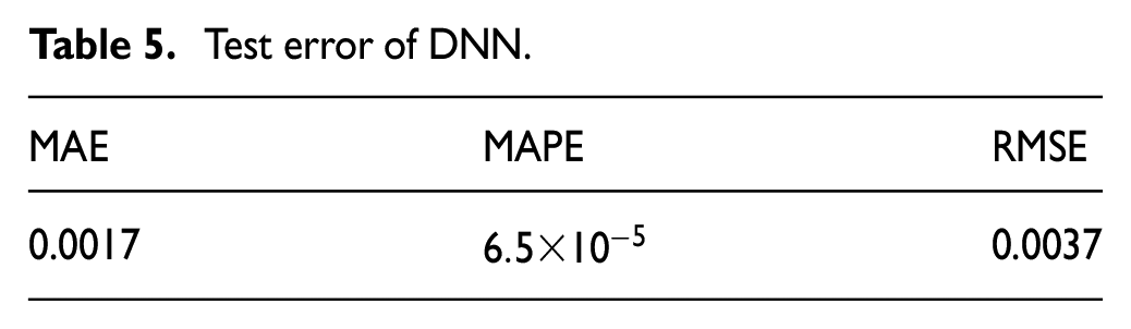
The convergence curve of the DNN is shown in Figure 11, with the number of iterations in abscissa and the training error in ordinate, which shows that the convergence is intact. This means that the dynamic model obtained is stable and reliable. In order to comprehensively represent the generalization ability of the DNN model in the test set, the network performance is evaluated in mean absolute error (MAE), mean absolute percentage error (MAPE), and root mean square error (RMSE), whose expressions are shown in Table 4.

Figure 11.

Training convergence curve of DNN.

Table 4.

List of different criteria.

Evaluating indicator	Expression
MAE	$\sum_{i = 1}^{N} \| {\hat{y}}_{i} - y_{i} \| / N$
MAPE	$\sum_{i = 1}^{N} (\| {\hat{y}}_{i} - y_{i} \| / y_{i}) / N$
RMSE	$\sqrt{\sum_{i = 1}^{N} {({\hat{y}}_{i} - y_{i})}^{2} / N}$

Table 5 shows the error of the DNN dynamic model in the test set. Its average percentage error is $6.5 \times 10^{- 5}$ , which can be considered to achieve high accuracy, while as shown in Figure 12, the MAE, MAPE, and RMSE of the DNN dynamic model are significantly smaller than the others, reflecting the superiority of DNN for the regression of complex and nonlinear data, which is conducive to the establishment of dynamic models with high accuracy.

Table 5.

Test error of DNN.

MAE	MAPE	RMSE
0.0017	$6.5 \times 10^{- 5}$	0.0037

Figure 12.

The error of the three models under different criteria.

Experimental modal test

Through the experimental modal test of the working platform-machine tool body system, the first six natural frequencies of sliding joints are obtained. The BK4525B three-direction accelerometer sensors and the Kistler 9724A2000 force hammer are adopted as experimental equipment. According to the experimental modal test principle in Figure 6, the experimental site is arranged as shown in Figure 13.

Figure 13.

Experimental modal test site.

The equivalent 3D model is established in the LMS analysis system, and the three-direction accelerometer sensors are placed discretely and evenly at the position corresponding to the measuring point diagram presented in Figure 14. A single-point excitation and multi-point collection method is used. Set point 21 as the excitation point and excite it with the force hammer, after which the signals of accelerometer sensors and excitation force are transmitted to the LMS analysis system. Its first six natural frequencies are finally presented in Table 6.

Figure 14.

The Establishment of the test model.

Table 6.

The first six natural frequencies of experimental modal test.

Order	1	2	3	4	5	6
Frequency (Hz)	17.868	32.408	121.928	152.381	254.185	282.239

Parameter identification

Based on the principle of equation (7), taking the 12 transversely isotropic virtual material parameters of the flat guide and the V-guide joints as optimization variables, taking the parameter range in Table 3 as the constraints, and taking the error between the experimental values and the predicted values of the DNN dynamic model as the objective function, the optimal identification model of the transversely isotropic virtual material parameters of the sliding joint is established as shown in equation (10).

\begin{matrix} min g (E_{τ p}, E_{np}, μ_{τ p}, μ_{np}, G_{np,} ρ_{p}, E_{τ v}, E_{nv}, μ_{τ v}, μ_{nv}, G_{nv,} ρ_{v}) \\ = \sqrt{\sum_{j = 1}^{6} | \frac{{f'}_{j} - f_{j}}{f_{j}} |} \\ s . t . 2.5 \times 1 0^{5} \leq E_{τ p} \leq 4 \times 10^{5} 3.5 \times 1 0^{4} \leq E_{np} \leq 6 \times 10^{4} \\ 0 \leq μ_{τ p} \leq 0.4 0 \leq μ_{np} \leq 0.4 \\ 1 \times 10^{5} \leq G_{np} \leq 1.5 \times 10^{5} 5000 \leq ρ_{p} \leq 9000 \\ 2.5 \times 1 0^{5} \leq E_{τ v} \leq 3.5 \times 10^{5} 1 \times 1 0^{5} \leq E_{nv} \leq 1.5 \times 10^{5} \\ 0 \leq μ_{τ v} \leq 0.4 0 \leq μ_{nv} \leq 0.4 \\ 8 \times 10^{4} \leq G_{nv} \leq 1.3 \times 10^{5} 5000 \leq ρ_{v} \leq 9000 \end{matrix}}

(10)

Where, $E_{τ p}, E_{np}, μ_{τ p}, μ_{np}, G_{np}, ρ_{p}$ are the virtual material parameters of the flat guide joint, and $E_{τ v}, E_{nv}, μ_{τ v}, μ_{nv}, G_{nv}, ρ_{v}$ are the virtual material parameters of the V-guide joints. $f'_{j}$ is the $j^{th}$ natural frequency predicted by the DNN dynamic model. $f_{j}$ is the $j^{th}$ natural frequency obtained from the experimental modal test.

The cuckoo search algorithm is applied to optimize the dynamic parameters of transversely isotropic virtual materials, whose convergence curve is presented in Figure 15.

Figure 15.

The parameters optimization convergence curve.

It can be seen that the results after 100 generations remain unchanged, indicating that the optimization has converged, which states that the global optimal solution has been found. The identified dynamic parameters are shown in Table 7.

Table 7.

Identification results for transversely isotropic virtual materials.

	Flat guide joint	V-guide joint
Tangential elastic modulus $E_{τ} (Pa)$	373976.469	331923.570
Normal elastic modulus $E_{n} (Pa)$	49660.967	149989.078
Tangential Poisson’s ratio $μ_{τ}$	0.206	0.002
Normal Poisson’s ratio $μ_{n}$	0.283	0.400
Normal shear modulus $G_{n} (Pa)$	129764.035	93141.167
Material density $ρ (kg / m^{3})$	8847.074	8121.838

The results acquired above are substituted into the FEA model for theoretical calculation. Then a comparison of the FEA calculated values with the experimental values is presented in Table 8, which shows that the percentage error of natural frequencies is minor in the first two orders, achieving 0.017% and 0.022%, respectively. The general error is less than 1%. It is better than the results in other literature and proves the validity of this method.

Table 8.

Error between FEA calculated values and experimental values.

Modal order	Experimental values of natural frequency (Hz)	Calculated values of finite element theory (Hz)	Percentage error (%)
1	17.87	17.871	0.017
2	32.41	32.415	0.022
3	121.93	121.12	0.663
4	152.38	152.38	0.001
5	254.19	254.69	0.199
6	282.24	283.4	0.411

Results and discussion

The spring damping and virtual material methods are the two most commonly used equivalent modeling methods for mechanical joints.⁴⁸ Spring damping method and virtual material method have their advantages and disadvantages. The spring damping method ignores the joint surface’s thickness and contact condition. Also, the different distribution forms of spring-damping elements and the number of elements have a great impact on the results, and meanwhile, it considers that each node is independent of the other, ignoring the coupling relationship at the joint.¹⁵ In contrast, the virtual material method takes into account thickness and roughness, mechanical properties, the processing technology of joints, and other factors. It includes the coupling relationship between each degree of freedom, but obtaining accurate material parameters is difficult.

In order to further verify the superiority of equivalent modeling based on transversely isotropic virtual material, the spring damping method and isotropic virtual material method are also applied for the equivalent modeling of the sliding joints of the working platform-machine tool body, both generating 11,000 sets of data sets and using DNN for dynamic modeling. The relative error between the theoretical and experimental values of the natural frequencies is used as an evaluation index for comparison. The final results are presented in Table 9.

Table 9.

Error comparison of the three equivalent modeling methods.

Order	Experimental values (Hz)	The relative error (%)
Order	Experimental values (Hz)	Spring damping method	Virtual material (isotropic)	Transversely isotropic material
1	17.87	0.817	0.101	0.017
2	32.41	0.549	0.207	0.022
3	121.93	0.236	0.778	0.663
4	152.38	0.104	0.216	0.001
5	254.19	0.450	0.195	0.199
6	282.24	0.503	0.482	0.411
Average value		0.443	0.330	0.219

A comprehensive comparison of the data in the table shows that the error of the three equivalent modeling methods is less than 1%, and the average error of the transversely isotropic virtual material method is the smallest of the three methods. Furthermore, the low-order natural frequencies error of the transversely isotropic virtual material method is significantly reduced. Its first-order error is reduced by 98% compared to the spring damping and 83% compared to the isotropic virtual material. The error from the second order is reduced by 96% and 89%, respectively, which can reflect the advantageousness of the transversely isotropic virtual material method. The first six mode shapes of the three equivalent modeling methods are shown in Table 10. By comparison, the first six mode shapes obtained by the three equivalent modeling methods are entirely the same. The similarity of the mode shapes of the three methods is very high. Combining the results of natural frequencies and mode shapes, the equivalent modeling based on transversely isotropic virtual material is reliable and has the highest accuracy.

Table 10.

The first six mode shapes of the three equivalent modeling methods.

Order	Spring damping method	Virtual material (isotropic)	Transversely isotropic material
1
2
3
4
5
6

Conclusion

This paper proposes a dynamic modeling method based on transversely isotropic virtual material and DNN for improving dynamic modeling accuracy and studies the sliding joints of the working platform-machine tool body system of a surface grinder. Firstly, the dynamic model reflecting the relationship between the transversely isotropic virtual material parameters and the FEA calculated theoretical natural frequencies is established by DNN. Then the optimization is carried out by utilizing the cuckoo search algorithm. The final parameter identification error is less than 1%, achieving high accuracy, proving this method’s effectiveness. Additionally, compared with the spring damping and isotropic virtual material methods, it is concluded that the equivalent modeling method of transversely isotropic virtual material has the best modeling accuracy.

The dynamic parameters identification method of the machine tool in this paper is not only suitable for the sliding joints of the working platform-machine tool body of the surface grinder but also for the parameter identification of other joints of the machine tool, which is universal and can be used for the overall dynamic analysis of the machine tool. In addition to the existing deep learning models and optimization algorithms, more deep learning models and optimization algorithms can be tried in future work to build dynamic and optimization models.

Footnotes

Handling Editor: Chenhui Liang

Declaration of conflicting interests

The author(s) declared no potential conflicts of interest with respect to the research, authorship, and/or publication of this article.

Funding

The author(s) disclosed receipt of the following financial support for the research, authorship, and/or publication of this article: This work is supported by the National Natural Science Foundation of China (Grant No. 51775323), and the Science and Technology Commission of Shanghai Municipality (Grant No. 17060502600).

ORCID iDs

Yichu Fan

Jianmin Zhu

References

Zhu

Luo

. Dynamic characteristics of guideway joints for CNC machine tool. AMM 2011; 80–81: 1051–1054.

Nie

. Analysis on dynamic characteristics of cnc machine tool and experiment with influence of rolling guide joint considered. AMR 2012; 443–444: 745–750.

Zhao

Zhang

, et al. Study on the dynamic characteristics of a virtual-axis hybrid polishing machine tool by flexible multibody dynamics. J Eng Manuf 2004; 218: 1067–1076.

Yang

Yuan

Wang

, et al. A prediction method for dynamic performance of machine tool joint surfaces. AMM 2013; 437: 8–12.

Frangoudis

Rashid

Nicolescu

. Development and analysis of a consciously designed Joint Interface Module for improvement of a machining system’s dynamic performance. Int J Adv Manuf Technol 2017; 88: 507–518.

Jiang

Hong

Chen

. Simplified dynamic modeling and model parameter identification of bolt-ed flange connection structure. Shock Vib 2020; 39: 170–175.

Wang

Shi

, et al. Virtual functional gradient material characterizes the dynamic characteristics of bolted joint. J Vib Eng Technol 2020; 33: 525–532.

Tian

. A novel complete analytic way to fixed machined joint. AMR 2011; 308–310: 527–30.

Han

Gong

, et al. Equivalent method of joint interface based on persson contact theory: virtual material method. Materials 2019; 12: 3150.

10.

Yan

Wang

, et al. Vibration and noise analysis of diesel engine based on virtual material modeling. Trans CSICE 2020; 38: 464–471.

11.

Shi

Zhang

Shi

, et al. Equivalent characteristic model of a rough contact interface based on virtual material method. Adv Mech Eng 2020; 14: 1–11.

12.

Huang

, et al. Virtual material parameter acquisition based on the basic characteristics of the bolt joint interface. Tribol Int 2016; 95: 109–117.

13.

Cui

Hua

, et al. Inverse identification of virtual material parameters using surface response methodology. Math Probl Eng 2018; 2018: 1–14.

14.

Qin

, et al. Dynamic modeling of tie-bolt rotors via fractal contact theory and virtual material method. Proc IMechE, Part C: J Mechanical Engineering Science 2022; 236: 5900–5915.

15.

Fishkis

Lin

. Formation and evolution of a subsurface layer in a metalworking process. Wear 1997; 206: 156–170.

16.

Gao

, et al. Modeling method based on nonlinear virtual material bolted joint dynamics. J Northeast Univ 2021; 42: 1111–1119.

17.

Liao

Zhang

Feng

, et al. Interface contact pressure-based virtual gradient material model for the dynamic analysis of the bolted joint in machine tools. J Mech Sci Technol 2016; 30: 4511–4521.

18.

Sun

Huang

Sun

, et al. Interface parameter identification of bolted connections based on gradient virtual material. Chin J Mech Eng 2018; 54: 102–109.

19.

Zhao

Wang

Yang

, et al. Constitutive relationship and finite element model of fixed joint based on transversely isotropic assumption. China Mech Eng 2016; 27: 1007–1011.

20.

Zha

Zhang

, et al. Modeling method for bolted joint interfaces based on transvers-ely isotropic virtual materials. AIM 2018; 2018: 1118–1123.

21.

Tian

. Dynamic modeling of virtual material at fixed joint of mechanical structure. Hubei: Huazhong University of Science and Technology, 2011.

22.

Lei

. Dynamic modeling, parameter identification and application of bolted joint based on contact characteristics. Hubei: Huazhong University of Science and Technology, 2016.

23.

Zhang

Wen

, et al. Fixed joint modeling method based on equivalent transversely isotropic virtual material. Chin J Mech Eng 2017; 53: 141–147.

24.

Guo

Yuan

Wang

, et al. Experimental study on dynamic stiffness of joint surface of sliding guide. China Mech Eng 2012; 23: 1021–1025.

25.

Wang

Yang

, et al. Research on macro-mesoscopic normal dynamic characteristics of sliding joint surface. Mech Syst Signal Pr 2018; 113: 156–167.

26.

Zong

Qin

Chu

. Modeling of frictional stick-slip of contact interfaces considering normal fractal contact. ASME J Appl Mech 2022; 89: 031003.

27.

Wang

Huang

Zhao

, et al. Finite element model of machine tool guideway joint. China Mech Eng 2004; 15: 1634–1636.

28.

Gao

Liu

. Dynamic modeling method of the bolted joint with uneven distribution of joint surface pressure. AIP Adv 2018; 8: 1–19.

29.

Bograd

Reuss

Schmidt

, et al. Modeling the dynamics of mechanical joints. Mech Syst Signal Pr 2011; 25: 2801–2826.

30.

Zhu

Zhou

, et al. Dynamic characteristic parameter identification of machine tool sliding joint surface based on neural network modeling. J Vib Shock 2018; 37: 109–115,131.

31.

Pan

, et al. New approach of friction model and identification for hydraulic system based on MAPSO-NMDS optimization Elman neural network. Adv Mech Eng 2017; 9: 1–14.

32.

Ryu

Noh

Kim

. Deep neural network based demand side short term load forecasting. Energies 2017; 10: 3.

33.

Pei

Hyun

Molinari

, et al. Finite element modeling of elastoplastic contact between rough surfaces. J Mech Phys Solids 2005; 53: 2385–2409.

34.

Ren

Wang

. Experimental study on the normal dynamic contact stiffness of guideway bond surface under lubrication condition. China Mech Eng 2018; 29: 811–816.

35.

Ding

Huang

Wang

, et al. Influence of nonlinearity of motion bond on the dynamic characteristics of large CNC machine tools. J Nanjing Tech Univ 2012; 34: 112–116.

36.

Starzynski

Buczkowski

. Ultrasonic Measurements of Contact Stiffness Between Rough Surfaces. ASME J Tribol 2014; 136: 34503.

37.

Janiesch

Zschech

Heinrich

. Machine learning and deep learning. Electron Mark 2021; 31: 685–695.

38.

Huang

Shao

Zhu

, et al. Tool wear condition monitoring across machining processes based on feature transfer by deep adversarial domain confusion network. J Intell Manuf 2023; 2023: 1–27.

39.

Zhu

Zhang

Huang

, et al. Identification of dynamic characteristic parameters of key joints of ball screw feeding system based on DNN whole machine modelling. J Vib Shock 2023; 42: 243–254+279.

40.

Zhang

Liu

Huang

, et al. Dynamic parameters identification for sliding joints of surface gri-nder based on deep neural network modeling. Adv Mech Eng 2021; 13: 1–15.

41.

Jia

Zhang

Wen

, et al. Joint surface modeling and parameter acquisition method based on virtual material. J Tyust 2013; 34: 347–351.

42.

Shrestha

Mahmood

. Review of deep learning algorithms and architectures. IEEE Access 2019; 7: 53040–53065.

43.

Alom

Taha

Yakopcic

, et al. A state-of-the-art survey on deep learning theory and architectures. Electronics 2019; 8: 292.

44.

Arpan

. Bio inspired computing – a review of algorithms and scope of applications. Expert Syst Appl 2016; 59: 20–32.

45.

Seif-Eddeen

Fateen

. Gradient-based cuckoo search for global optimization. Math Probl Eng 2014; 493740: 1–12.

46.

Gandomi

Yang

Alavi

. Cuckoo search algorithm: a metaheuristic approach to solve structural optimization problems. Eng Comput 2013; 29: 17–35.

47.

Yuan

, et al. Influence of spatial position of double turntable swing on dyna-mic characteristics of five-axis machine tool. Adv Mech Eng 2022; 14: 1–15.

48.

Cai

Wang

, et al. Research progress in dynamic characteristics of bolted joints. Chin J Mech Eng 2013; 49: 158–168.

Dynamic modeling of sliding joints based on transversely isotropic virtual material and deep neural network

Abstract

Keywords

Introduction

Basic principle

Equivalent modeling of sliding joints

Establishment of the DNN dynamic model

Experimental modal test

Identification of dynamic parameters

Equivalent modeling of sliding joints based on transversely isotropic virtual material

Establishment of the DNN dynamic model

Experimental modal test

Identification of transversely isotropic virtual material parameters

Application case study

Establishment of the FEA model

Establish the geometric model including the sliding joints

Set basic material parameters

Set parameters of transversely isotropic virtual material

Constraints and meshing

Establishment of the DNN model

Data set generation

Model design

Model training

Experimental modal test

Parameter identification

Results and discussion

Conclusion

Footnotes

Declaration of conflicting interests

Funding

ORCID iDs

References