Sage Journals: Discover world-class research

Abstract

In order to ensure that safety and reliability of tractor semitrailer combinations (TSCs) on the road, the human drivers’ steering decisions need to comprehensively consider the trajectories and states of the tractor and semitrailer. For this purpose, a dual predictive model adaptive switching control decision for directional control is proposed. Firstly, a multi-point preview algorithm and a general regression neural network are designed to percept the current local target paths for the tractor and semitrailer. Then, a kinematic predictive model control algorithm for low-speed path tracking control and a dynamic predictive model control algorithm for high-speed path following and lateral stability control are established respectively. In addition, an S-type switching function is introduced to realize smooth switching between the two control algorithms. Finally, the directional control decision in this study is validated by the numerical simulations under different conditions and compared with single-point preview driver and the MPC driver without considering semitrailer. The results show that the proposed approach can accurately track the target path and effectively improve the high-speed lateral stability.

Keywords

Trailer semitrailer combination (TSC)MPC path following lateral stability

Introduction

Tractor-semitrailer combination (TSC) consists of a powered unit, namely tractor, and one towed unit, called semitrailer, which are connected each other by a fifth where or dolly. As the most typical articulated heavy vehicle (AHV), it plays a vital role in the development of economy and logistics industry.^1,2 However, two unique disadvantages of poor low-speed maneuverability and low high-speed stability often cause tragic traffic accidents.³ And, many accidents are caused by human drivers’ misjudgment and wrong operation.^4,5 Better understanding human driver behaviors can more realistically simulate some situations in actual driving, which is very essential for the development of chassis control system and autonomous system of AHVs.⁶

In recent years, the research on active safety of AHVs is mainly focused on active trailer steering^7–10 and differential braking.^11–13 And various driver models, such as single-point preview PID control,¹⁴ single-point preview optimal control,¹⁵ multi-point preview optimal control,¹⁶ adaptive control,¹⁷ fuzzy control,¹⁸ and sliding-mode control,¹⁹ are used to build “driver-AHV-road” closed-loop system to verify the control effect. These models are actually the driver models of single unit vehicles, which can well realize the path tracking of tractors. However, trailers are completely ignored, they cannot really simulate the behavior of articulated vehicle drivers.

In reality, the steering behavior of AHV drivers is quite different from that of single unit vehicle drivers. Most AHV drivers are professional drivers, who are aware of the configuration and performance of their vehicles. Moreover, an AHV driver’s input is governed by his/her comprehensive reaction to the tractor and trailer behavior.²⁰ Such as, when driving on narrow or large curvature roads, the drivers can simultaneously predict and plan the driving paths of tractor and trailer to avoid the trailer leaving lane and collision accidents. And they have ability to prevent excessive yaw of the trailer and avoid rollover at high-speed.

Up to now, there are few research reports on the study of AHV drivers’ behaviors. Based on “preview-follow” theory proposed by Guo and Fancher,²¹ Li et al.²² developed a quasi-linear driver model and analyzed the effects of driver’s time delay, semitrailer load, and driving speed on TSC stability. Oreh et al.²³ proposed a desired articulation angle for directional control of the articulated vehicles, and based on this, designed a fuzzy control driver model to simulate the steering behaviors. Rigatos et al.²⁴ studied the nonlinear optimal control method for truck-trailer direction control basing on iterative solution of Riccati equation. Guan et al.²⁵ established a kinematics model to predict the trajectory of the tractor and designed a MPC control algorithm to follow the target path. Yun et al.²⁶ developed a MPC driver model by using the separate axis theorem to simulate the TSC driver’s steering behavior on the narrow and large curvature road. However, these driver models mentioned above did not comprehensively take the tracking and states of the trailer into consideration, which are difficult to more realistically simulate the steering behavior of human drivers. Oliveira et al.²⁰ proposed an optimal path planning method based on kinematics model to analyze driver’s behavior, but driver’s preview process and the trailer’s lateral stability at high-speed were ignored.

Based on the forgoing studies, this paper aims to establish a driver model comprehensively considering the trajectories and states of the tractor and semitrailer to simulate the human driver’s behavior. As a systematic controller, the driver model consists two parts, longitudinal velocity control and directional control. In velocity control, the accelerator/brake pedal is uniformly determined by a linear discrete PID controller according to the error of longitudinal speed. In directional control, on one hand, not only the off-tracking of the tractor and the semitrailer, but also the lateral stability of the semitrailer at high-speed should be considered. On the other hand, the dynamics of low-speed large turning angle and high-speed small turning angle are very different,^14,27 which cannot be ignored. That is to say, it is very difficult for any predictive control basing on a single model to meet the requirements. Fortunately, multi-model adaptive switching control can effectively solve this problem.

Therefore, a dual model adaptive switching controller is proposed to realize the direction control of TSC. Based on “preview-follow” theory, the driver’s steering behavior is divided into three processes: firstly, perceive the road environment and anticipate the target path. Multi-point preview algorithm can easily and quickly obtain the path information and has been widely used in the driver model.^28,29 Based on multi-point preview thought, this paper presents a perception algorithm to obtain tractor target path based on forward preview and trailer target path based on backward preview. Moreover, these few discrete points are not enough to clearly describe the target paths of the tractor and semitrailer. The general regression neural network (GRNN) with good non-linear approximation performance is especially suitable for solving curve fitting problem.³⁰ Compared with other methods (BP network, Spline Curve), it has no weight, high calculating speed and the curve fitting is very natural.³¹ Thus, the GRNN fitting method is adopted to fitting TSC’s target paths in this paper. Secondly, predict the future trajectories and states of the tractor and semitrailer. To overcome the problem that a single model is difficult to accurately predict the trajectories and states at different speeds, the low-speed kinematic and high-speed dynamic predictive models are established to predict the trajectories and states of the tractor and trailer. Finally, a dual model adaptive prediction control algorithm is designed to track the anticipated target paths.

This paper organized as follows. The forward and backward multi-point preview algorithm and the target path fitting method based on GRNN are described in section “Target path perception process.” On this basis, the two MPC controllers based on kinematics and dynamics model and an S-style switch function between them are introduced in section “Directional controller design.” The simulation results and analysis under different conditions are described in section “Numerical Test Simulations and Discussions.” Finally, the conclusions are given in section “Conclusion.”

Target path perception process

Due to the lengthy TSC, the trajectory of the semitrailer always deviates greatly from that of the tractor. The TSC drivers have very good driving skills, can predict in advance and make corresponding operations to avoid that the tractor can pass the curve smoothly while the trailer cannot or rollover. To simulate this behavior of the human driver, the first thing to do is percept the road information, especially the path of the road.

Typically, the sample but effective method to describe an arbitrary path is the use of path coordinate table. Any road can be described approximately by using enough discrete coordinates on the path. The coordinates in the table are accurate, and other points can be obtained by data interpolation or curve fitting.²⁹ Therefore, this paper divides the target path perception into two steps. First, the sparse target points for the tractor and semitrailer are obtained by forward and backward previewing respectively. Then, the more precise target paths are fitted by GRNN network. The detail process is described in the following subsection.

Forward and backward preview

According to the above description, the forward and backward multi-point preview process is presented in Figure 1. For the convenience of calculations, it is assumed that the driver is located in the middle of the front axle of the tractor.

Figure 1.

The forward and backward multi-point preview process.

As shown in Figure 1, the TSC consists of a three-axle tractor and a three-axle semitrailer. Suppose the current driver’s position in ground coordinate is (x_d, y_d), and the target point corresponding to the current driver’s position is (x_p₀, y_p₀), which is also the cut-off point of forward and backward preview. The farthest distance of the forward preview is determined by the preview time and tractor longitudinal velocity, and the farthest point of backward preview is the center of the second axle of the semitrailer. So the preview distances can be easily expressed as follow,

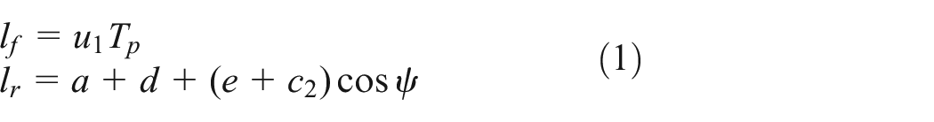
\begin{matrix} l_{f} = u_{1} T_{p} \\ l_{r} = a + d + (e + c_{2}) \cos ψ \end{matrix}

(1)

where, u₁ is the longitudinal velocity of the tractor, T_p is the preview time, a is the distance from the first axle to the centroid of tractor, d is the distance from centroid of the tractor to the fifth wheel, e is the distance from the fifth wheel to the centroid of the semitrailer, c₂ is the distance from the centroid of the semitrailer to its second axle. ψ is the folding angle between the tractor and the semitrailer.

The other preview points are equidistant along the preview direction, and the coordinates of these preview points {x_p, y_p} used to define the local target path are expressed as,

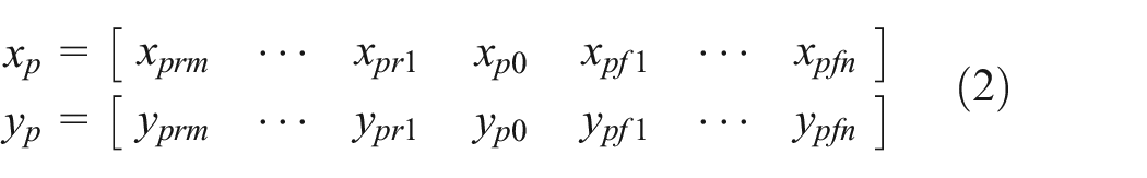
\begin{matrix} \begin{matrix} x_{p} = [\begin{matrix} \begin{matrix} x_{prm} & \dots & x_{pr 1} \end{matrix} & x_{p 0} & \begin{matrix} x_{pf 1} & \dots & x_{pfn} \end{matrix} \end{matrix}] \\ y_{p} = [\begin{matrix} \begin{matrix} y_{prm} & \dots & y_{pr 1} \end{matrix} & y_{p 0} & \begin{matrix} y_{pf 1} & \dots & y_{pfn} \end{matrix} \end{matrix}] \end{matrix} \end{matrix}

(2)

where, m, n are the number of forward and backward preview points, respectively. In this study, the values of the variable m and n are chosen as m = 2 and n = 5.

Target path fitting based on GRNN network

To get the precise target path within the preview range, the driver’s preview points described in subsection “Forward and backward preview” can be obtained by closed-loop simulation using the driver model embedded in TruckSim. At the same time, the driver’s preview time T_p, tractor’s longitudinal velocity u₁ and the steering angle $δ_{f}$ are also recorded. And then, these preview information is used to fit the local target path based on GRNN network.

The GRNN consists of four layers, which are the input layer, the radial basis layer, the additive layer and the output layer. As show in Figure 2, $x = {[\begin{matrix} \begin{matrix} x_{p} & δ_{f} \end{matrix} & \begin{matrix} T_{p} & u_{1} \end{matrix} \end{matrix}]}^{T}$ is used as input quantity and $y = y_{p}$ is used as output quantity.

Figure 2.

The GRNN network structure.

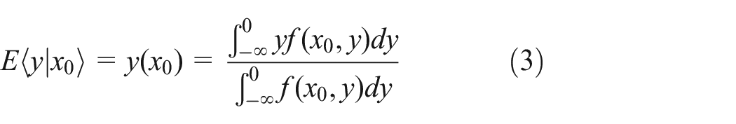
The theoretical basis of GRNN is mainly nonlinear regression, it’s another variation of radial basis neural network. Suppose f(x, y) is the probability density function of the random variables of x and y. If the observed value of x is known to be x₀, the regression of y with respect to x is

E 〈 y | x_{0} 〉 = y (x_{0}) = \frac{\int_{- \infty}^{0} yf (x_{0}, y) dy}{\int_{- \infty}^{0} f (x_{0}, y) dy}

(3)

If the sample data set {x_i, y_i} i = 1, 2,…n, using the Parzen nonparametric estimation, the density function f(x₀, y) can be estimated as follows

f (x_{0}, y) = \frac{1}{n {(2 π)}^{\frac{p + 1}{2}}} \sum_{i = 1}^{n} e^{- d (x_{0}, x_{i})} e^{- d (y_{0}, y_{i})}

(4)

where, $d (x_{0}, x_{i}) = \sum_{j = 1}^{p} {[(x_{0 j} - x_{ij}) / σ]}^{2}, d (y, y_{i}) = {[y - y_{i}]}^{2}$ , n is the sample size and p is the dimension of random variable x.

If replacing f(x₀, y) by the estimated probability density function and exchanging the order of integration and summation, there is

y (x_{0}) = \frac{\sum_{i = 1}^{n} e^{- d (x_{0}, x_{i})} \int_{- \infty}^{+ \infty} y e^{- d (y_{0}, y_{i})} dy}{\sum_{i = 1}^{n} e^{- d (x_{0}, x_{i})} \int_{- \infty}^{+ \infty} e^{- d (y_{0}, y_{i})} dy}

(5)

Because $\int_{- \infty}^{+ \infty} x e^{- x^{2}} dx = 0$ , by simplifying the above formula to obtain

y (x_{0}) = \frac{\sum_{i = 1}^{n} y e^{- d (y_{0}, y_{i})}}{\sum_{i = 1}^{n} e^{- d (y_{0}, y_{i})}}

(6)

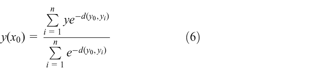
where, the numerator is weighted sum of the y_i values calculated to train samples.

In order to verify the fitting effect, the simulations under conditions of S-turn at low-speed and lane change at high-speed are used to collect the samples of preview information. During the simulations, the samples are taken every 0.01 s, and 80% of the collected samples are randomly selected for GRNN network training, and the remaining data are verified. Then the trained GRNN is used to reconstruct the local target path, and compared with B-spline fitting path.

The preview points, the road centerline, the local target path based on GRNN fitting, and the local target path based on B-spline interpolation at one point in time under two conditions are respectively shown in Figures 3(a) and 4(a). And, the lateral error between the target path and the road centerline are illustrated in Figures 3(b) and 4(b), respectively. It can be clearly seen that the local target paths obtained by the two methods are consistent with the road centerline, and the lateral error based on GRNN fitting is smaller than that based on B-spline interpolation. This indicates that the GRNN fitting method is better than B-spline interpolation method.

Figure 3.

Fitting results under S-turn at low-speed: (a) target trajectory and (b) lateral error.

Figure 4.

Fitting results under lane change at high-speed: (a) target trajectory and (b) lateral error.

Ultimately, to implement the subsequent path tracking control algorithm, it is necessary to sample the specific target points of the tractor and semitrailer from the fitted target path. To facilitate sampling, the variable of distance along the target path called as station is introduced. The station (S) is a spatial independent variable. For any given value of S, there is a unique sequence of X and Y coordinates. The corresponding increment of S is computed by using the Pythagorean theorem.

S_{i} = S_{i - 1} + \sqrt{{(x_{gi} - x_{g (i - 1)})}^{2} + {(y_{gi} - y_{g (i - 1)})}^{2}}, 1 < i < n

(7)

where, x_g and y_g are coordinates of the target path points fitted by GRNN network. n is the number of these points, the value is larger, the precision of the target path is higher.

The starting point of the target path of the tractor and semitrailer are points (x₀, y₀) and (x_rm, y_rm), respectively. The distance intervals of the tractor and semitrailer along the target path can be expressed as,

\begin{matrix} Δ s_{i} = T_{s} \sqrt{{(u_{i} + v_{i})}^{2}} & i = 1, 2 \end{matrix}

(8)

where, u₁ and u₂ are the longitudinal speeds of the tractor and semitrailer, respectively. v₁ and v₂ are the lateral speeds of the tractor and semitrailer, respectively. And, T_s is the sample time. So, the final path point set η_ref can be easily gained by equal interval sampling.

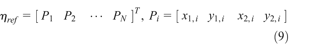
η_{ref} = {[\begin{matrix} \begin{matrix} P_{1} & P_{2} \end{matrix} & \begin{matrix} \dots & P_{N} \end{matrix} \end{matrix}]}^{T}, P_{i} = [\begin{matrix} \begin{matrix} x_{1, i} & y_{1, i} \end{matrix} & \begin{matrix} x_{2, i} & y_{2, i} \end{matrix} \end{matrix}]

(9)

where, N is the prediction horizon for the model predictive control algorithm. The subscripts 1 and 2 indicate the tractor and semitrailer, respectively.

The point set η_ref is the target paths followed by the direction control of subsequent driver model.

Directional controller design

In this part, a dual model adaptive switching controller is mainly established to track the target path described in Section “Target path perception process.” As shown in Figure 5, the low-speed KMPC (kinematic model predictive control) controller is designed based on yaw plane kinematic model to minimize the lateral path deviation of the tractor and semitrailer at low-speed. And the high-speed DMPC (dynamic model predictive control) controller is built based on yaw plane dynamic model to minimize the lateral path deviation of the tractor and semitrailer and improve lateral stability at high-speed. In addition, a smooth S-type function is introduced as switching function to avoid transient response of switch process and achieve model switching smoothly. The detail process is described in the following subsection.

Figure 5.

The structure of directional control based on MPC.

Low-speed KMPC controller

Based on the principle of MPC,³² it is necessary to establish an internal model of the low-speed KMPC controller to predict the trajectories of the tractor and semitrailer. So, a simplified yaw plane kinematics model is derived in this study. It is assumed that the suspension, steering system, and influence of lateral dynamics of TSC are ignored. And, the steering angle of the front wheel for the tractor is taken as the steering input.

As shown in Figure 6, δ₁ represents the steering angle of front axle wheel for the tractor, o_i (i = 1, 2) is the instantaneous center of speed for the tractor and semitrailer, respectively. u_i and v_i (i = 1, 2) represent the longitudinal and lateral velocities of the tractor and semitrailer, respectively. ψ_i represents the yaw angle of the tractor and semitrailer, respectively. ψ is the folding angle between the tractor and semitrailer. Equations for the motion of the tractor and semitrailer can be described as:

\begin{matrix} {\begin{matrix} \begin{matrix} {\overset{\cdot}{x}}_{1} = u_{1} \cos ψ_{1} - v_{1} \sin ψ_{1} \\ {\overset{\cdot}{y}}_{1} = u_{1} \sin ψ_{1} + v_{1} \cos ψ_{1} \end{matrix} \\ \begin{matrix} {\overset{\cdot}{x}}_{2} = u_{2} \cos ψ_{2} - v_{2} \sin ψ_{2} \\ {\overset{\cdot}{y}}_{2} = u_{2} \sin ψ_{2} + v_{2} \cos ψ_{2} \end{matrix} \end{matrix} \end{matrix}

(10)

Figure 6.

Yaw plane kinematic model for TSC.

According to the Ackerman steering relationship, the relationships between the yaw rate, lateral velocity, and front axle steering angle for the tractor can be expressed as:

{\overset{\cdot}{ψ}}_{1} = \frac{u_{1} \tan δ_{1}}{a + (b_{1} + b_{1}) / 2}

(11)

v_{1} = \frac{(b_{1} + b_{2}) u_{1} \tan δ_{1}}{2 a + (b_{1} + b_{2})}

(12)

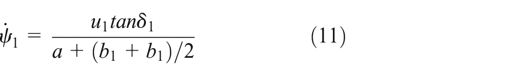
where, b₁ and b₂ are the distance from the centroid of the tractor to the two rear axles respectively.

Based to the kinematic constraints between the tractor and semitrailer. The motion of the semitrailer can be easy deduced as:

\begin{matrix} {\overset{\cdot}{ψ}}_{2} = \frac{u_{1} \sin ψ + (v_{1} - d {\overset{\cdot}{ψ}}_{1}) \cos ψ}{e + c_{2}} \\ u_{1} = u_{1} \cos ψ - (b - d) {\overset{\cdot}{ψ}}_{1} \sin ψ \\ v_{1} = u_{1} \sin ψ + (b - d) {\overset{\cdot}{ψ}}_{1} \cos ψ - e {\overset{\cdot}{ψ}}_{2} \end{matrix}

(13)

where, d is the distance from fifth wheel to the centroid of the tractor, e is the distance from fifth wheel to the centroid of the semitrailer, c₂ is the distance from the fifth axel to the centroid of the semitrailer. The folding angle ψ = ψ₁−ψ₂. By combining equations (10)–(13), the general form of the complete kinematic model for the TSC at low-speed can be obtained as:

\overset{\cdot}{X} = f (X, U)

(14)

where, the state vector $X = {[\begin{matrix} ψ_{1} & ψ_{2} & x_{1} & y_{1} & x_{2} & y_{2} \end{matrix}]}^{T}$ , and control input $U = δ_{1}$ .

The approximated linear system acquired by ignoring the high-order term of Taylor series expansion for equation (14). And, the trajectories of tractor and semitrailer as the output of predictive model can be given by

\begin{matrix} \overset{\cdot}{X} = A (t) X + B (t) U + Γ \\ Y = CX \end{matrix}

(15)

where, t is the current time, the time varying coefficient matrices A(t), B(t), and the constant matrix C are listed in Appendix A, the correction value between the internal predictive model and the plant model are given by

Γ = F (X_{t}, U_{t}) - A (t) X_{t} - B (t) U_{t}

(16)

Where, F(X_t, U_t) is the first derivative of the state vector of plant model for the TSC and used to correct the outputs of the predictive model at current time.

To facilitate the numerical calculation, assuming that the sampling time is T_s, the discretization the above predictive model is performed as:

{\begin{matrix} X (t + T_{s}) = A_{d} (t) X_{t} + B_{d} (t) U_{t} + T_{s} A_{d} (t) Γ \\ Y (t + T_{s}) = CX (t + T_{s}) \end{matrix}

(17)

where, $A_{dt} = e^{A (t) T}$ , $B_{dt} = \int_{0}^{T} e^{A (t) τ} B (t) d τ$

It can be found from equation (17) that the internal predictive model is a linear time-varying (LTV) system. In order to facilitate the design of LTV-MPC controller, the predictive model needs to be converted into incremental input form.

{\begin{matrix} ξ (k + 1 | t) = A_{k, t} ξ (k | t) + B_{k, t} Δ U (k | t) + Λ_{k, t} \\ Y (k | t) = C_{k, t} ξ (k | t) \end{matrix}

(18)

where, ξ(k + 1, t) is the new state vector, which contains the control input vector and original state vector, it is expressed as:

ξ (k | t) = [\begin{matrix} X (k | t) \\ U (k - 1 | t) \end{matrix}]

(19)

where, k is the prediction step.

According to the model predictive control principle, the coming position for the tractor and semitrailer are predicted based on equation (18). In a prediction horizon, the change of the longitudinal velocity is very small and assumed as constant. In addition, to reduce the complexity of controller design, it is assumed that the prediction system is time invariant in each prediction horizon. So the coefficient matrices can be expressed as:

A_{k, t} = A_{k - 1, t} = \dots A_{t} = [\begin{matrix} A_{d} (t) & B_{d} (t) \\ 0_{1 \times 5} & 1 \end{matrix}]

(20)

B_{k, t} = B_{k - 1, t} = \dots B_{t} = [\begin{matrix} B_{d} (t) \\ 1 \end{matrix}]

(21)

C_{k, t} = C_{k - 1, t} = \dots C_{t} = [\begin{matrix} C & 0_{4 \times 1} \end{matrix}]

(22)

Λ_{k, t} = Λ_{k - 1, t} = \dots Λ_{t} = [\begin{matrix} Γ (t) \\ 1 \end{matrix}]

(23)

If the prediction horizon and control horizon of MPC are N_p and N_c, and N_c < N_p. At the time step t, the output vectors during prediction horizon would be

η (t) = [\begin{matrix} \begin{matrix} ξ (t + 1 | t) \\ ξ (t + 2 | t) \\ ⋮ \end{matrix} \\ \begin{matrix} ξ (t + N_{c} | t) \\ ⋮ \\ ξ (t + N_{p} | t) \end{matrix} \end{matrix}]

(24)

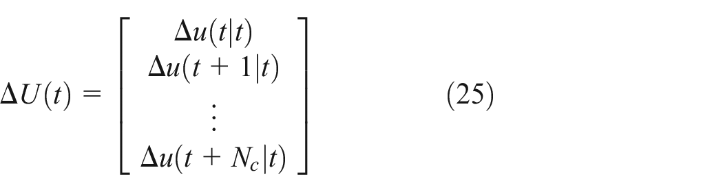
Meanwhile, the control input vectors during the control horizon would be

Δ U (t) = [\begin{matrix} \begin{matrix} Δ u (t | t) \\ Δ u (t + 1 | t) \end{matrix} \\ \begin{matrix} ⋮ \\ Δ u (t + N_{c} | t) \end{matrix} \end{matrix}]

(25)

At the time step t, if the state vector ξ(k + 1, t), the control input vector ΔU(t), the coefficient matrices A_d (t), B_d (t), and the correction value Γ(t) are known, the predicted output vectors are derived as:

η (t) = Ψ_{t} ξ (k | t) + Θ_{t} Δ U (k | t) + Φ_{t}

(26)

where,

\begin{matrix} Ψ_{t} = [\begin{matrix} \begin{matrix} C_{t} A_{t} \\ C_{t} A_{t}^{2} \\ ⋮ \end{matrix} \\ \begin{matrix} C_{t} A_{t}^{N_{c}} \\ ⋮ \\ C_{t} A_{t}^{N_{p}} \end{matrix} \end{matrix}], \\ Θ_{t} = [\begin{matrix} \begin{matrix} C_{t} B_{t} & 0 \\ C_{t} A_{t} B_{t} & C_{t} B_{t} \end{matrix} & \begin{matrix} 0 & 0 \\ 0 & 0 \end{matrix} \\ \begin{matrix} ⋮ & ⋮ \\ C_{t} A_{t}^{N_{c} - 1} B_{t} & C_{t} A_{t}^{N_{c} - 2} B_{t} \end{matrix} & \begin{matrix} ⋱ & ⋮ \\ \dots & C_{t} B_{t} \end{matrix} \\ \begin{matrix} ⋮ & ⋮ \\ C_{t} A_{t}^{N_{p} - 1} B_{t} & C_{t} A_{t}^{N_{p} - 2} B_{t} \end{matrix} & \begin{matrix} ⋱ & ⋮ \\ \dots & C_{t} A_{t}^{N_{p} - N_{c} - 1} B_{t} \end{matrix} \end{matrix}], \end{matrix}

Φ_{t} = [\begin{matrix} \begin{matrix} C_{t} Λ \\ C_{t} A_{t} Λ + C_{t} Λ \\ ⋮ \end{matrix} \\ \begin{matrix} C_{t} A_{t}^{N_{c} - 1} Λ + C_{t} A_{t}^{N_{c} - 2} Λ + \dots + C_{t} Λ \\ ⋮ \\ C_{t} A_{t}^{N_{p} - 1} Λ + C_{t} A_{t}^{N_{p} - 2} Λ + \dots + C_{t} Λ \end{matrix} \end{matrix}]

As mentioned above, the objective of the low-speed controller is to make decision of the front wheel angle enable the TSC to track the target path smoothly and to reduce the off-tracking of the semitrailer. Therefore, the objective function is minimize the lateral deviations between target path and the trajectories of the tractor and the semitrailer. And, the method of quadratic programming is used to solving the control input. The objective function of the design is as follows

\begin{matrix} J (k) = \sum_{i = 1}^{N_{P}} ‖ η (k + 1 | t) - η_{ref} (k + 1 | t) ‖_{Q}^{2} \\ + \sum_{i = 1}^{N_{c}} ‖ Δ u (k + 1 | t) ‖_{R}^{2} + ρ ε^{2} \end{matrix}

(27)

where, Q and R are weight matrices, N_p is the prediction time domain (N_p = 24), T_c is the control time domain (N_c = 10), ρ is the relaxation coefficient (ρ = 1), and ε² is the relaxation variable. The first and second factors respectively stand for the ability of system following target path and the constraint of variable changes. Then, the objective function can be transformed into a general optimization problem with multi constraints and the optimal control vector sequence $Δ U$ can be calculated to minimize the error between the predicted trajectories and the target path.

The control quantity limit constraint and the incremental control constraint are the main constraint forms considered in this article. The expressed form of the control quantity is as follows

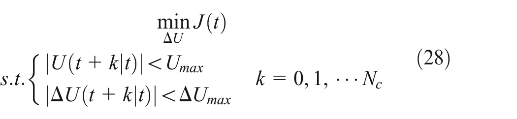
\begin{matrix} \begin{matrix} min_{Δ U} J (t) \\ \begin{matrix} s . t . {\begin{matrix} | U (t + k | t) | < U_{\max} \\ | Δ U (t + k | t) | < Δ U_{\max} \end{matrix} & k = 0, 1, \dots N_{c} \end{matrix} \end{matrix} \end{matrix}

(28)

where, U_max and ΔU_max are the limits of the front wheel angle and front wheel angle increment, which presents the driver steering operation limits.

After solving the above optimization problem, the first elements of $Δ U (t + k | t)$ will be used to calculate the controller output at current time t. At next time, the new optimization will be solved over a shifted prediction again with updated state $ξ (t)$ correction value $Λ_{t}$ and local planning path η_ref.

High-speed DMPC controller

In order to improve the path following ability and lateral stability of the tractor and semitrailer at high-speed. This part is mainly to establish model predictive controller based on linear yaw plane dynamic model.

Based on the above design process of low-speed KMPC controller, a linear yaw plane dynamic model is established to predict the driving trajectories and status of tractor and semitrailer. As shown in Figure 7, F_yi (i = 1, 2…6) are the tire lateral forces for the tractor and semitrailer. F_yt is the reaction force of the fifth wheel on the tractor and semitrailer.

Figure 7.

Linear dynamic model for TSC.

It is assumed that the pitch and bounce motions are ignored. In addition, the front wheel angle of the tractor and the folding angle between the tractor and trailer is small. So, $\sin (δ_{1}) \approx δ_{1}$ , $\sin (ψ) \approx ψ$ , and equations representing the motion of the tractor and semitrailer can be written as:

\begin{matrix} \begin{matrix} m_{1} ({\overset{\cdot}{v}}_{1} + u_{1} {\overset{\cdot}{ψ}}_{1}) = F_{y 1} \cos δ_{1} + F_{y 2} + F_{y 3} - F_{yt} \\ I_{z 1} {\overset{\cdot\cdot}{ψ}}_{1} = a F_{y 1} \cos δ_{1} - b_{1} F_{y 2} - b_{2} F_{y 3} + d F_{yt} \end{matrix} \\ \begin{matrix} m_{2} ({\overset{\cdot}{v}}_{2} + u_{2} {\overset{\cdot}{ψ}}_{2}) = F_{yt} \cos ψ + F_{y 4} + F_{y 5} + F_{y 6} \\ I_{z 2} {\overset{\cdot\cdot}{ψ}}_{2} = e F_{yt} \cos ψ - c_{1} F_{y 4} - c_{2} F_{y 5} - c_{3} F_{y 6} \end{matrix} \end{matrix}

(29)

where, m₁ and m₂ are the total mass of the tractor and the semitrailer, respectively. Iz₁ and Iz₂ are the moment of inertia about the yaw axis for the tractor and semitrailer, respectively.

Because the front wheel angle of the tractor is small when driving at high-speed. The tire cornering stiffness is assumed in the linear region. So the linear relationship between the tire lateral force and the tire sideslip angle can be described as:

\begin{matrix} \begin{matrix} F_{y 1} = k_{1} (\frac{v_{1} + a {\overset{\cdot}{ψ}}_{1}}{u_{1}} - δ_{1}) \\ F_{y 2} = k_{2} \frac{v_{1} - b_{1} {\overset{\cdot}{ψ}}_{1}}{u_{1}} \end{matrix} \\ \begin{matrix} F_{y 3} = k_{3} \frac{v_{1} - b_{2} {\overset{\cdot}{ψ}}_{1}}{u_{1}} \\ F_{y 3 + i} = k_{3 + i} \frac{v_{2} - c_{i} {\overset{\cdot}{ψ}}_{2}}{u_{2}}, i = 1, 2, 3 \end{matrix} \end{matrix}

(30)

where k₁, k₂, and k₃ are the cornering stiffness of the wheels for the tractor, respectively. k₄, k₅, and k₆ are the cornering stiffness of the rear wheels for the semitrailer, respectively.

Similarly, with a small front wheel angle, the folding angle between the tractor and the semitrailer is also very small. So the kinematic constraint equation between the tractor and the trailer can be described as:

\begin{matrix} u_{2} = u_{1} - (b - d) {\overset{\cdot}{ψ}}_{1} ψ \\ v_{2} = u_{1} ψ - (b - d) {\overset{\cdot}{ψ}}_{1} - e {\overset{\cdot}{ψ}}_{2} \end{matrix}

(31)

Furthermore, the relationship between the tractor yaw rate and the semitrailer yaw rate is

\overset{\cdot}{ψ} = {\overset{\cdot}{ψ}}_{1} - {\overset{\cdot}{ψ}}_{2}

(32)

By eliminating the coupling reaction F_yt from equation (29) and considering equations (30) and (31), the state space form of TCS dynamic equations can be expressed as equation (33). In equation (33), the lateral velocity of the tractor CG, the yaw rates, and angles of the tractor and semitrailer are taken as the state variables.

\overset{\cdot}{X} = M^{- 1} AX + M^{- 1} BU

(33)

where, X is the state variable vector, M, A, and B are matrixes listed in Appendix B.

By combing the equation (10), the augmented state equation in the same form as equation (17) can be expressed as

{\begin{matrix} X (t + T_{s}) = A_{d} (t) X_{t} + B_{d} (t) U_{t} + T_{s} A_{d} (t) Γ \\ Y (t + T_{s}) = CX (t + T_{s}) \end{matrix}

(34)

where, $X = {[\begin{matrix} \begin{matrix} v_{1} & {\overset{\cdot}{ψ}}_{1} & {\overset{\cdot}{ψ}}_{2} \end{matrix} & \begin{matrix} ψ_{1} & ψ_{2} & x_{1} \end{matrix} & \begin{matrix} y_{1} & x_{2} & y_{2} \end{matrix} \end{matrix}]}^{T}$ , $U = δ$ . A(t), B(t), and C are matrixes listed in Appendix C.

By using the same method as the kinematic model, the model (34) is discretized as

{\begin{matrix} X (t + T_{s}) = A_{d} (t) X_{t} + B_{d} (t) U_{t} + T_{s} A_{d} (t) Γ \\ Y (t + T_{s}) = CX (t + T_{s}) \end{matrix}

(35)

Next, based on model (35), the trajectories, yaw rates, and lateral accelerations of the tractor and semitrailer at high-speed can be predicted, and this calculation process is exactly the same as the above low-speed KMPC controller, so the derivation process is not repeated here.

In addition, to simplify calculations, the objective function of the high-speed controller is consistent with that of the low-speed controller, but their constraint conditions are different. In order to give consideration to the lateral stability of the TSC, not only the amplitude and speed of the driver steering operation but also the yaw rates of the tractor and semitrailer are constrained. Therefore, the steering input at high-speed can be obtained by optimizing equation:

\begin{matrix} min_{Δ U} J (t) \\ \begin{matrix} s . t . {\begin{matrix} \begin{matrix} | U (t + k | t) | < U_{\max} \\ | Δ U (t + k | t) | < Δ U_{\max} \end{matrix} \\ | r (t + k | t) | < r_{\max} \end{matrix} & k = 0, 1, \dots, N_{c} \end{matrix} \end{matrix}

(36)

where, r_max is the limit value of the yaw rates for the tractor and semitrailer. The lateral acceleration of vehicle is actually a superposition of the yaw motion and lateral translation, and yaw motion contributes far more than lateral translation. According to Wang et al.,³³ the limit value of the yaw rate is defined as

r_{max} = \frac{0.85 a_{y max}}{u}

(37)

where, a_ymax is the rollover threshold, which is obtained by the following simulation test.

Finally, the front wheel angle for the tractor at high-speed can be obtained by solving the optimization problem (36).

S-style switch function

As mentioned above, the S-style switch function is used to realize smooth switching between the above two sub controllers. The key to design the switch function is to select the reasonable switching points. In general, the linear yaw plane dynamic model is suitable for the condition of the small front wheel angle and small folding angle, usually less than 10°. To obtain the limit steering angle for TSC at different speeds, the simulations of circular test with different front wheel angles are carried out.

During the simulation tests, the TSC travels in a straight line at the initial speed of 10 km/h. At some point, an angle step input is directly input at the front wheel of the tractor. When the steady state steering is reached, the tractor starts to accelerate at a very low acceleration until the TSC reaches the maximum speed or rollover occurs. Record the roll angles of the semitrailer and lateral accelerations at the centroid of the tractor and semitrailer, and then, increase the amplitude of the angle step and repeat the simulation.

Figure 8(a) to (c) show the changes of the roll angle, lateral accelerations with front wheel angle, and longitudinal velocity, respectively. It can be seen that when the velocity is higher than 25 km/h, there is possibility of rollover. And the rollover threshold of the tractor is about 0.463 g, and that of the semitrailer is about 0.406 g. In addition, when the longitudinal velocity is higher than 35 km/h, the limit angle of front wheel of the tractor is less than 10°.

Figure 8.

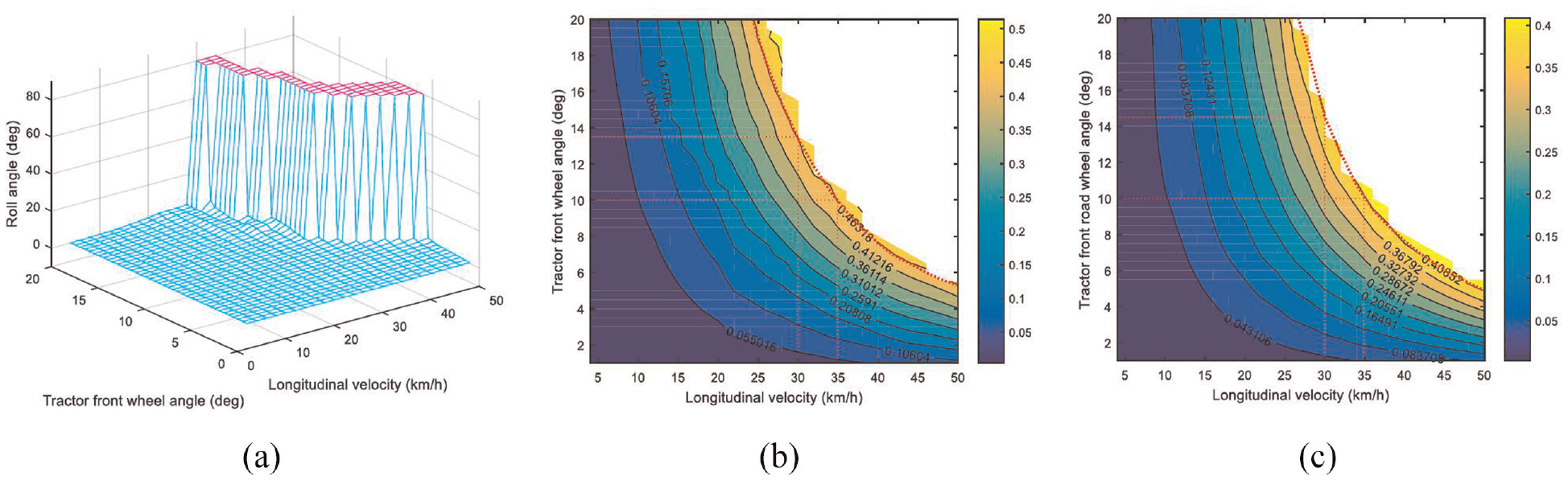
The results of the steady-state steering: (a) roll angle of trailer, (b) lateral acceleration of mass center for the tractor, and (c) lateral acceleration of mass center for the semitrailer.

Based on the above analysis, the longitudinal velocity is divided into three zone: low-speed zone (u < 30 km/h), high-speed zone (u > 40 km/h), and transition zone. In the low-speed zone, only the low-speed KMPC controller is executed. And in the high-speed zone, only the DMPC controller is executed. To realize smooth switching between the two controllers, the S-style switch function about longitudinal velocity is expressed as

w_{c} (u) = {\begin{matrix} 0, & u \leq 30 \\ 2 {(\frac{u - 30}{5})}^{2}, & 30 < u < 35 \\ 1 - 2 {(\frac{u - 40}{5})}^{2}, & 35 \leq u < 40 \\ 1, & u \geq 35 \end{matrix}

(38)

Finally, the direction control of the driver model are developed by integrating target path perception algorithm, KMPC sub controller, DMPC sub controller, and S-style switch function.

Numerical test simulations and discussions

In order to verify the driver model proposed in this article and discuss the effects of path tracking and lateral stability, the co-simulation platform is established based on TruckSim and Matlab/Simulink. A high fidelity TSC model as the controlled object is established in TruckSim. And, the driver model is presented in Simulink.

Based on the co-simulation platform, three scenarios of the right angle turn at low-speed, S-turn at moderate-speed, and double lane change at high-speed are carried out. The path tracking effect is analyzed and discussed from the trajectories of the centers of the first axle, third axle, and sixth axle. The reason for choosing the trajectories at the center of these axles is that they can better illustrate the path tracking effect than the trajectories at the centroid of the tractor and semitrailer. And, the lateral stability is discussed from the lateral accelerations of the tractor and semitrailer. In addition, for further comparative analysis, a single-point preview driver model and a MPC driver model without considering semitrailer are established to compare with the driver model proposed in this article. The TSC model parameters in this study are shown in Table 1.

Table 1.

The parameter value for the TSC model.

Notation	Value	Unit
a/b₁/b₂	2.335/1.164/2.434	m
c₁/c₂/c₃	1.1/2.3/3.5	m
d/e	1.799/5.599	m
m₁/m₂	6595/25,910	kg
I_Z1/I_Z2	45,075/285,368	kg m²
k₁/k₂/k₃	−123,330/−121,152/−121,152	N/rad
k₄/k₅/k₆	−130,097	N/rad

Right-angle turn test

Right-angle turn with a 90° curve is very useful to assess the path-tracking performance of TSC’s driver. During the test, the longitudinal velocity of the tractor is kept at a constant speed of 8 km/h, and the simulation results are shown in Figure 8.

Figure 9 shows the road centerline and the trajectories at the center of the first, third, and sixth axles under right angle turn test. It is easy to see that there are obvious differences in the tracking effect of these three drivers. For the single-point preview driver, the tractor travels along inside of the curve. As a result, the rear axle of the semitrailer seriously deviates from the road centerline, especially at the top of the right angle, the maximum transient off-tracking is as high as 5.73 m, which seriously run out lane. The MPC driver without considering semitrailer can drive the tractor along the road centerline, but compared with the driver proposed in this paper, the trailer still has relatively large off tracking. Only the driver considering the semitrailer can drive the tractor along the outside of the curve to avoid that the semitrailer deviates seriously from the road centerline, which is consistent with the steering behavior of the human driver. Moreover, the maximum off-tracking for the semitrailer reduces to 2.5 m, which is more than 55% lower than that of the single-point driver. This implies that the driver model proposed in this article has the best path tracking on narrow or large curvature road.

Figure 9.

The trajectories at the center of the first, third, and sixth axles under right angle turn test: (a) single-point preview driver, (b) MPC driver without considering semitrailer, and (c) driver proposed in this article.

S-turn test

S-turn test is used to simulate the steering behavior when the TSC drive at moderate-speed. During the test, the longitudinal velocity of tractor is maintained at a constant speed of 35 km/h. In this case, both the low-speed controller and high-speed controller are involved.

Figures 10(a) to 12(a) provide very useful results for analyzing the path following effect under S-turn condition. It can be seen from Figures 10(a) and 11(a) that for the single-point preview driver and the MPC driver without considering semitrailer, the trajectories at the center of the first, third, and sixth axles are all distributed on the inside of the curve and the off-tracking phenomena are amplified from front to rear. And the tracking effect of the MPC driver is significantly better than that of the single-point driver. However, Figure 12(a) illustrates that the trajectories of the first and third axles are outside of the road centerline, and the trajectory of the sixth axle is inside of the road center line. Hence, the driver model proposed in this paper has the best path tracking ability than the other two driver models.

Figure 10.

The simulation results for the single-point driver under the S-turn test: (a) the trajectories at the center of the first, third, and sixth axles and (b) lateral accelerations of the tractor and the semitrailer.

Figure 11.

The simulation results for the MPC driver without considering semitrailer under the S-turn test: (a) the trajectories at the center of the first, third, and sixth axles and (b) lateral accelerations of the tractor and the semitrailer.

Figure 12.

The simulation results for the driver proposed in the article under the S-turn test: (a) the trajectories at the center of the first, third, and sixth axles and (b) lateral accelerations of the tractor and the semitrailer.

Figures 10(b) to 12(b) show the lateral accelerations at the mass center of the tractor and the semitrailer. It can be seen that the peak value of lateral acceleration increases with the improvement of the path tracking effect. Nevertheless, for the driver based on dual predictive model adaptive switching control, the peak values of the both lateral accelerations are less than 0.3g, far lower the rollover thresholds. This indicates that the driver model proposed in this article can improve the path tracking ability and maintain good lateral stability for TSC at medium-speed.

Double lane change test

Double lane change test is very useful to verify the lateral stability of TSCs at high-speed. During this test, the longitudinal velocity of tractor is kept at 80 km/h. In this case, only the high-speed controller works.

Figures 13(a) to 15(a) provide useful simulation results for analyzing whether the TSC can follow the road centerline accurately at high-speed. Compare with the single-point preview driver and MPC driver without considering semitrailer, the driver model proposed in this article has the best path following performance. The maximum lateral deviation from the road centerline is 0.31 m, decreasing 68.6% from the corresponding single-point preview driver model of 1.05 m, and decreasing 23.2% from the corresponding MPC driver model without considering semitrailer of 0.434 m.

Figure 13.

The simulation results for the single-point driver under the double lane change test: (a) the trajectories at the center of the first, third, and sixth axles and (b) lateral accelerations of the tractor and the semitrailer.

Figure 14.

The simulation results for the MPC driver without considering semitrailer under the double lane change test: (a) the trajectories at the center of the first, third, and sixth axles and (b) lateral accelerations of the tractor and the semitrailer.

Figure 15.

The simulation results for the driver proposed in the article under the double lane change test: (a) the trajectories at the center of the first, third, and sixth axles and (b) lateral accelerations of the tractor and the semitrailer.

Figures 12(b) to 14(b) show the accelerations at the tractor and the semitrailer CGs under high-speed double lane change test. And the acceleration peak values of the tractor and semitrailer are illustrated in Table 2. It can be seen that for the driver model proposed in this article, the peak values of the accelerations are obviously smaller than that of the other two drivers. Those imply that the driver proposed in this article can effectively improve the TSC’s path following ability and latera stability at high-speed.

Table 2.

The acceleration peak values for the tractor and semitrailer: (Driver a) single-point preview driver; (Driver b) MPC driver without considering the semitrailer; (Driver c) driver proposed in this article.

Driver model	Peak value of lateral acceleration for tractor (g)	Peak value of lateral acceleration for semitrailer (g)
Driver a	0.31/−0.378	0.286/−0.338
Driver b	0.248/−0.36	0.272/−0.328
Driver c	0.247/−0.345	0.245/−0.321

Conclusions

Based on the methods of multi-point preview and the GRNN nonlinear fitting to perceive the target path, this article establishes a dual predictive model adaptive switching control driver model to comprehensively consider the trajectory for the tractor and semitrailer. Simulation analysis is performed, and it is compared with the single-point preview driver model and MPC driver model without considering semitrailer. The results show that the driver model based on dual predictive model adaptive switching control can better track the target path and effectively improve the lateral stabiliy at high-speed.

Footnotes

Appendix A: Relevant matrixes definition

State space matrices for the TCS kinematic model

\begin{matrix} \overset{\cdot}{X} = A (t) X + B (t) U + Γ \\ Y = CX \end{matrix}

Where, A(t), B(t), and Γ are matrixes and they are defined as:

A (t) = [\begin{matrix} 0 & 0 & 0 & 0 & 0 & 0 \\ A_{2, 1} & A_{2, 2} & 0 & 0 & 0 & 0 \\ A_{3, 1} & 0 & 0 & 0 & 0 & 0 \\ A_{4, 1} & 0 & 0 & 0 & 0 & 0 \\ A_{5, 1} & A_{5, 2} & 0 & 0 & 0 & 0 \\ A_{6, 1} & A_{6, 2} & 0 & 0 & 0 & 0 \end{matrix}]

A_{2, 1} = \frac{- (b - d) u_{1} \sin (ψ_{1} - ψ_{2})}{L_{1} L_{2}} \tan δ_{1} + \frac{u_{1} \cos (ψ_{1} - ψ_{2})}{L_{2}}

A_{2, 2} = \frac{(b - d) u_{1} \sin (ψ_{1} - ψ_{2})}{L_{1} L_{2}} \tan δ_{1} - \frac{u_{1} \cos (ψ_{1} - ψ_{2})}{L_{2}}

\begin{matrix} A_{3, 1} = - u_{1 t} \sin ψ_{1 t} - \frac{b u_{1 t} \tan δ_{1 t} \cos ψ_{1 t}}{L_{1}}, A_{4, 1} = u_{1 t} \cos ψ_{1 t} - \frac{b u_{1 t} \tan δ_{1 t} \sin ψ_{1 t}}{L_{1}} \end{matrix}

\begin{matrix} A_{5, 1} = \cos ψ_{2 t} [- u_{1 t} \sin (ψ_{1 t} - ψ_{2 t}) - \frac{(b - d) u_{1 t} \cos (ψ_{1 t} - ψ_{2 t}) \tan δ_{1 t}}{L_{1}}] \\ - \sin ψ_{2 t} [\frac{u_{1 t} \cos (ψ_{1 t} - ψ_{2 t}) (L_{2} - e)}{L_{2}} - \frac{(L_{2} - e) (b - d) u_{1} \sin (ψ_{1} - ψ_{2}) \tan δ_{1}}{L_{1} L_{2}}] \end{matrix}

\begin{array}{l} A_{5, 2} = \cos ψ_{2 t} [u_{1 t} \sin (ψ_{1 t} - ψ_{2 t}) + \frac{(b - d) u_{1 t} \cos (ψ_{1 t} - ψ_{2 t}) \tan δ_{1 t}}{L_{1}}] - \sin ψ_{2 t} \\ [- \frac{u_{1 t} \cos (ψ_{1 t} - ψ_{2 t}) (L_{2} - e)}{L_{2}} + \frac{(L_{2} - e) (b - d) u_{1} \sin (ψ_{1} - ψ_{2}) \tan δ_{1}}{L_{1} L_{2}}] \\ - \sin ψ_{2 t} [u_{1} \cos (ψ_{1} - ψ_{2}) - (b - d) \sin (ψ_{1} - ψ_{2}) \frac{u_{1} \tan δ_{1}}{L_{1}}] \\ - \cos ψ_{2 t} [\frac{u_{1} \sin (ψ_{1} - ψ_{2}) (L_{2} - e)}{L_{2}} + \frac{(L_{2} - e) (b - d) u_{1} \cos (ψ_{1} - ψ_{2}) \tan δ_{1}}{L_{1} L_{2}}] \end{array}

\begin{matrix} A_{6, 1} = \sin ψ_{2 t} [- u_{1 t} \sin (ψ_{1 t} - ψ_{2 t}) - \frac{(b - d) u_{1 t} \cos (ψ_{1 t} - ψ_{2 t}) \tan δ_{1 t}}{L_{1}}] \\ + \cos ψ_{2 t} [\frac{u_{1 t} \cos (ψ_{1 t} - ψ_{2 t}) (L_{2} - e)}{L_{2}} - \frac{(L_{2} - e) (b - d) u_{1} \sin (ψ_{1} - ψ_{2}) \tan δ_{1}}{L_{1} L_{2}}] \end{matrix}

\begin{matrix} A_{6, 2} = \sin φ_{2 t} [u_{1 t} \sin (ψ_{1 t} - ψ_{2 t}) + \frac{(b - d) u_{1 t} \cos (ψ_{1 t} - ψ_{2 t}) \tan δ_{1 t}}{L_{1}}] \\ + \cos ψ_{2 t} [- \frac{u_{1 t} \cos (ψ_{1 t} - ψ_{2 t}) (L_{2} - e)}{L_{2}} + \frac{(L_{2} - e) (b - d) u_{1} \sin (ψ_{1} - ψ_{2}) \tan δ_{1}}{L_{1} L_{2}}] \\ + \cos ψ_{2 t} [u_{1} \cos (ψ_{1} - ψ_{2}) - (b - d) \sin (ψ_{1} - ψ_{2}) \frac{u_{1} \tan δ_{1}}{L_{1}}] \\ - \sin ψ_{2 t} [\frac{u_{1} \sin (ψ_{1} - ψ_{2}) (L_{2} - e)}{L_{2}} + \frac{(L_{2} - e) (b - d) u_{1} \cos (ψ_{1} - ψ_{2}) \tan δ_{1}}{L_{1} L_{2}}] \end{matrix}

B_{1, 1} = \frac{u_{1 t}}{L_{1} \cos^{2} δ_{1 t}}, B_{2, 1} = \frac{(b - d) u_{1 t} \cos (ψ_{1 t} - ψ_{2 t})}{L_{1} L_{2} \cos^{2} δ_{1 t}}, B_{3, 1} = - \frac{b u_{1 t} \sin ψ_{1 t}}{L_{1} \cos^{2} δ_{1 t}}, B_{4, 1} = \frac{b u_{1 t} \cos ψ_{1 t}}{L_{1} \cos^{2} δ_{1 t}}

B_{5, 1} = - \cos ψ_{2 t} (b - d) \sin (ψ_{1 t} - ψ_{2 t}) \frac{u_{1 t}}{L_{1} \cos^{2} δ_{1 t}} - \sin ψ_{2 t} \frac{(L_{2} - e) (b - d) u_{1 t} \cos (ψ_{1 t} - ψ_{2 t})}{L_{1} L_{2} \cos^{2} δ_{1 t}}

B_{6, 2} = - \sin ψ_{2 t} (b - d) \sin (ψ_{1 t} - ψ_{2 t}) \frac{u_{1 t}}{L_{1} \cos^{2} δ_{1 t}} + \cos ψ_{2 t} \frac{(L_{2} - e) (b - d) u_{1 t} \cos (ψ_{1 t} - ψ_{2 t})}{L_{1} L_{2} \cos^{2} δ_{1 t}}

\overset{\cdot}{X} = [\begin{matrix} \begin{matrix} 0 & 0 & 1 \\ 0 & 0 & 0 \end{matrix} & \begin{matrix} 0 & 0 & 0 \\ 1 & 0 & 0 \end{matrix} \\ \begin{matrix} 0 & 0 & 0 \\ 0 & 0 & 0 \end{matrix} & \begin{matrix} 0 & 1 & 0 \\ 0 & 0 & 1 \end{matrix} \end{matrix}]

Appendix B: Relevant matrixes definition

State space matrices for the TCS dynamic model

\overset{\cdot}{X} = M^{- 1} AX + M^{- 1} BU

Where, M, A, and B are matrixes and they are defined as:

M = [\begin{matrix} d m_{1} & 0 & 0 & 0 & 0 \\ m_{1} + m_{2} & - d m_{2} & - e m_{2} & 0 & 0 \\ e m_{1} & 0 & I z_{2} & 0 & 0 \\ 0 & 0 & 0 & 1 & 0 \\ 0 & 0 & 0 & 0 & 1 \end{matrix}], A = [\begin{matrix} S_{11} & S_{12} & 0 & 0 & 0 \\ S_{21} & S_{22} & S_{23} & S_{24} & S_{25} \\ S_{31} & S_{32} & S_{33} & S_{34} & S_{35} \\ 0 & 1 & 0 & 0 & 0 \\ 0 & 0 & 1 & 0 & 0 \end{matrix}]

S_{11} = \frac{(a + d) k_{1}}{u_{1}} + \frac{(d - b_{1}) k_{2}}{u_{1}} + \frac{(d - b_{2}) k_{3}}{u_{1}}, S_{12} = - m_{1} d u_{1} + \frac{(a + d) a k_{1}}{u_{1}} - \frac{(d - b_{1}) b_{1} k_{2}}{u_{1}} - \frac{(d - b_{2}) b_{2} k_{3}}{u_{1}}

S_{21} = \frac{k_{1} + k_{2} + k_{3}}{u_{1}} + \frac{k_{4} + k_{5} + k_{6}}{u_{2}}, S_{22} = \frac{a k_{1} - b_{1} k_{2} - b_{2} k_{3}}{u_{1}} - \frac{d k_{4} + d k_{5} + d k_{6}}{u_{2}} - (m_{1} + m_{2}) u_{1}

S_{23} = - \frac{(c_{1} + e) k_{4}}{u_{2}} - \frac{(c_{2} + e) k_{5}}{u_{2}} - \frac{(c_{3} + e) k_{6}}{u_{2}} - m_{2} (u_{1} - u_{2}), S_{24} = \frac{(k_{4} + k_{5} + k_{6}) u_{1}}{u_{2}}

S_{25} = - \frac{(k_{4} + k_{5} + k_{6}) u_{1}}{u_{2}}, S_{31} = \frac{e (k_{1} + k_{2} + k_{3})}{u_{1}} - \frac{c_{1} k_{4} + c_{2} k_{5} + c_{3} k_{6}}{u_{2}}

S_{32} = - \frac{e (a k_{1} - b_{1} k_{2} - b_{2} k_{3})}{u_{1}} + \frac{d (c_{1} k_{4} + c_{2} k_{5} + c_{3} k_{6})}{u_{2}} - e m_{1} u_{1}, S_{33} = \frac{c_{1} (c_{1} + e) k_{4}}{u_{2}} + \frac{c_{2} (c_{2} + e) k_{5}}{u_{2}} + \frac{c_{3} (c_{3} + e) k_{6}}{u_{2}}

S_{34} = - \frac{(c_{1} k_{4} + c_{2} k_{5} + c_{3} k_{6}) u_{1}}{u_{2}}, S_{35} = \frac{(c_{1} k_{4} + c_{2} k_{5} + c_{3} k_{6}) u_{1}}{u_{2}}, B = {[\begin{matrix} - (a + d) k_{1} & - k_{1} & - e k_{1} & 0 & 0 \end{matrix}]}^{T}

Appendix C: Relevant matrixes definition

State space matrices for the TCS dynamic model

\overset{\cdot}{X} = A (t) X + B (t) U + Γ

Where, A(t), and B(t) are matrixes and they are defined as:

A (t) = [\begin{matrix} M^{- 1} A & 0_{5 \times 4} \\ Ξ & 0_{4 \times 4} \end{matrix}]

Ξ = [\begin{matrix} - \sin (ψ_{1}) & 0 & - u_{1} \sin (ψ_{1}) - v_{1} \cos (ψ_{1}) & 0 & 0 \\ \cos (ψ_{1}) & 0 & u_{1} \cos (ψ_{1}) - v_{1} \sin (ψ_{1}) & 0 & 0 \\ - \sin (ψ_{2}) & d \sin (ψ_{2}) & e \sin (ψ_{2}) & - u_{1} \sin (ψ_{2}) & p_{1} \\ \cos (ψ_{2}) & - d \cos (ψ_{2}) & - e \sin (ψ_{2}) & u_{1} \cos (ψ_{2}) & p_{2} \end{matrix}]

P_{1} = - u_{2} \sin (ψ_{2}) - [u_{1} (ψ_{1} - ψ_{2}) + v_{1} - d {\overset{\cdot}{ψ}}_{1} - e {\overset{\cdot}{ψ}}_{2}] \cos (ψ_{2}) + u_{1} \sin (ψ_{2})

P_{1} = - u_{2} \cos (ψ_{2}) - [u_{1} (ψ_{1} - ψ_{2}) + v_{1} - d {\overset{\cdot}{ψ}}_{1} - e {\overset{\cdot}{ψ}}_{2}] \sin (ψ_{2}) + u_{1} \cos (ψ_{2})

B (t) = [\begin{matrix} M^{- 1} B \\ 0_{4 \times 1} \end{matrix}], C = Diag ([\begin{matrix} 0 & 1 & 1 & 0 & 0 & 0 & 1 & 1 & 1 & 1 \end{matrix}])

Handling Editor: Chenhui Liang

Author contributions

Xiaobing, Chen conceived of the study, carried out the directional control algorithm for TSC and drafted the manuscript. Qiang, Yao participated in its design and coordination and helped to draft the manuscript. All authors read and approved the final manuscript.

Declaration of conflicting interests

The author(s) declared no potential conflicts of interest with respect to the research, authorship, and/or publication of this article.

Funding

The author(s) disclosed receipt of the following financial support for the research, authorship, and/or publication of this article: This work is supported by the Foundation for Young Scholars of Hubei province, China (Q20170813) and Foundation of Hubei Collaborative Innovation Center, China (2015XTZX0412).

Ethical approval/patient consent

Written informed consent for publication of this paper was obtained from the Hubei University of automotive technology and all authors. Human or animal subjects and pathological reports were not involved in this study.

ORCID iD

Chen Xiaobing

References

Odhams

Roebuck

Cebon

, et al. Dynamic safety of active trailer steering systems. Proc IMechE, Part K: J Multi-body Dynamics 2008; 222: 367380.

Islam

Ding

. A closed-loop dynamic simulation based design method for articulated heavy vehicles with active trailer steering systems. Veh Syst Dyn 2012; 50: 675–697.

El-Gindy

Mrad

Tong

. Sensitivity of rearward amplification control of a truck/full trailer to tyre cornering stiffness variations. Proc IMechE, Part D: J Automobile Engineering 2001; 215: 579–588.

Han

Zhao

Chang

. Driver behaviour and traffic accident involvement among professional heavy semi-trailer truck drivers in China. PLoS One 2021; 16: e0260217.

Elhemly

MAE

Fayed

MAG

. Simulation of tractor semitrailer manoeuvre at high speed using Matlab/Simulink. Int J Heavy Veh Syst 2011; 14: 341–358.

Félez

García-Sánchez

Lozano

. Control design for an articulated truck with autonomous driving in an electrified highway. IEEE Access 2018; 6: 60171–60186.

Kural

Hatzidimitris

van

Wouw

. Active trailer steering control for high-capacity vehicle combinations. IEEE Trans Intell Veh 2017; 2: 251–265.

Sorge

. A nonlinear dynamical approach to the path correction of multi-steering articulated vehicles. Veh Syst Dyn 2021; 59: 1759–1780.

Zhang

Jiang

. Active control on path following and lateral stability for truck–trailer combinations. Arab J Sci Eng 2019; 44: 1365–1377.

10.

Wang

. A study on single lane-change manoeuvers for determining rearward amplification of multitrailer articulated heavy vehicles with active trailer steering systems. Veh Syst Dyn 2016; 54: 128–149.

11.

Sun

. Design synthesis of car-trailer systems with active trailer differential braking strategies. Master Thesis, The University of Ontario Institute of Technology, Ontario, Canada, 2013.

12.

Sun

Lee

. Non-linear bifurcation stability analysis for articulated vehicles with active trailer differential braking systems. SAE Int J Mater Manuf 2016; 9: 688–698.

13.

Mobini

Ghaffari

Alirezaei

. Non-linear optimal control of articulated-vehicle planar motion based on braking utilizing the state-dependent Riccati equation method. Proc IMechE, Part D: J Automobile Engineering 2015; 229: 1744–1787.

14.

Zhang

Jiang

, et al. Active control on path following and lateral stability for truck-trailer combinations. Arab J Sci Eng 2019; 44: 1365–1377.

15.

Islam

. Design of a preview controller for articulated heavy vehicles. J Mech Eng Autom 2013; 3: 662–676.

16.

. Design and validation of a robust active trailer steering system for multi-trailer articulated heavy vehicles. Veh Syst Dyn 2018; 57: 1545–1571.

17.

Keymasi Khalaji

Moosavian

SAA

. Robust adaptive controller for a tractor-trailer mobile robot. IEEE/ASME Trans Mechatron 2014; 19: 943–953.

18.

Sahin

Akalin

. Articulated vehicle lateral stability management via active rear-wheel steering of tractor using fuzzy logic and model predictive control. SAE Int J Commer Veh 2020; 13: 115–128.

19.

Esmaeili

. An adaptive sliding mode controller for the lateral control of articulated long vehicles. Proc IMechE, Part K: J Multi-body Dynamics 2019; 233: 487–515.

20.

Oliveira

Ljungqvist

Lima

, et al. Optimization-based on-road path planning for articulated vehicles. IFAC-PapersOnLine 2020; 53: 15572–15579.

21.

Guo

Fancher

. Preview-follower method for modelling closed-loop vehicle directional control. In: Proceeding of the 19th annual conference on manual control Massachusetts, Cambridge, Massachusetts, 1983, pp.159–186.

22.

Zhang

Wang

. Driving stability of closed loop tractor-semitrailer vehicle system with optimal driver model. In: International conference on measuring technology and mechatronics automation, Zhangjiajie, China, 11–12 April 2009, pp.514–517. New York: IEEE.

23.

Oreh

SHT

Kazemi

Azadi

. A new desired articulation angle for directional control of articulated vehicles. Proc IMechE, Part K: J Multi-body Dynamics 2012; 226: 298–314.

24.

Rigatos

Siano

Wira

. A nonlinear H-infinity control approach for autonomous truck and trailer systems. Unmanned Syst 2020; 8: 49–69.

25.

Guan

Kim

Wang

. Comprehensive path and attitude control of articulated vehicles for varying vehicle conditions. Int J Heavy Veh Syst 2017; 24: 65–95.

26.

Yun

Yang

Huh

. Development of a narrow passage driving system for semi-trailer truck by using MPC. Int J Automot Technol 2022; 23: 785–791.

27.

Tabatabaei

Kazemi

Azadi

. A new desired articulation for directional control of articulated vehicle. Proc IMechE, Part K: J Multi-body Dynamics 2012; 226: 298–314.

28.

Guo

Huang

, et al. Research on path-tracking control method of intelligent vehicle based on adaptive two-point preview. SAE Int J Connected Autom Veh 2021; 4: 189–204.

29.

Sharp

. Driver steering control and a new perspective on car handling qualities. Proc IMechE, Part C: J Mechanical Engineering Science 2005; 21: 1041–1051.

30.

Jiang

Tian

Hua

. Model predictive driver model considering the steering characteristics of the skilled drivers. Adv Mech Eng 2019; 11: 1–14.

31.

Baker

. Can flexible non-linear modeling tell us anything new about educational productivity? Econ Educ Rev 2001; 20: 81–92.

32.

Mayne

. Optimization in model predictive control. Methods Model Based Process Control 1995; 293: 367–396.

33.

Wang

Chen

Zhao

. Application study of active front steering with integrated feedback steering-by-wire system. Int J Mech Syst Eng 2013; 3: 148–153.

Dual predictive model adaptive switching control for directional control of tractor semitrailer combinations

Abstract

Keywords

Introduction

Target path perception process

Forward and backward preview

Target path fitting based on GRNN network

Directional controller design

Low-speed KMPC controller

High-speed DMPC controller

S-style switch function

Numerical test simulations and discussions

Right-angle turn test

S-turn test

Double lane change test

Conclusions

Footnotes

Appendix A: Relevant matrixes definition

Appendix B: Relevant matrixes definition

Appendix C: Relevant matrixes definition

Author contributions

Declaration of conflicting interests

Funding

Ethical approval/patient consent

ORCID iD

References