Sage Journals: Discover world-class research

Abstract

An adaptive metamodel-based global approximation (AMGA) method for solving the global approximation problem of black-box models in large design domain is proposed in this study. The method employs the RBF model to compute the Hessian matrix and a heuristic direct search algorithm DIRECT to find the maximum curvature point of the metamodel surface, through which the design domain is split to obtain additional sampling points and to achieve fast update and fast valuation of the metamodel. The initial design domain is split into a series of sub-design domains by continuous iterations, and the metamodels built within the various sub-design domains achieve the global approximate model of the entire design domain. To demonstrate the final effect of the global approximation model and design domain splitting, six common two-dimensional test functions are chosen. The AMGA method is further tested using seven typical test functions and compared to other sampling and metamodel updating methods, with the findings demonstrating the usefulness of the proposed method in the low-dimensional scenario (less than four variables). Finally, the AMGA method is applied to a sophisticated electric car model, yielding good results.

Keywords

Black-box function metamodel adaptive ERBF model curvature

Introduction

Shortening the product design development cycle has gradually become a focus of attention in order to meet the harsh market rivalry as the design of electromechanical devices becomes increasingly sophisticated. The product design cycle can be considerably shortened by building and analyzing the simulation model of electromechanical items. However, as product complexity grows, simulation analysis consumes more and more computational resources. To address this issue, metamodeling approaches were developed and implemented in a variety of industries,^1–3 including aerospace, cars, and ships. The computational complexity is effectively decreased by creating a high-precision metamodel of the original complex model and replacing it for simulation analysis and optimization.

The metamodel is built with sampling points. A variety of sampling methods can be used to collect sampling points, which are classified into three types: classical sampling, full-space sampling, and adaptive sampling methods.⁴ To complete the collection of sampling points in the design domain, traditional and full-space sampling methods require a single sampling. Traditional sampling, also known as edge distribution sampling, distributes sampling points at the design domain’s boundaries, whereas spatial sampling can sample the whole design domain. In general, it is not acceptable to build a metamodel all at once; if too many points are sampled, the construction process is time-consuming and may affect utilization; if too few points are sampled, the built metamodel is not accurate enough to match the application requirements. Furthermore, because the nature of the source model is unknown, determining the appropriate sampling method is difficult. The adaptive sampling method is used to generate the metamodel as a solution to this challenge. Adaptive sampling is a new sampling method based on classical sampling and full-space sampling, with the key idea being to estimate the sparsity of sampling points based on the extent of the error between the approximation and the genuine value. This strategy divides the sampling procedure into numerous stages rather than completing the entire experimental design in a single sampling phase, and the subsequent sampling is based on the prior one.

Many methods for adaptive sampling and metamodel updating have been proposed in recent years. The Sequential Exploratory Experimental Design (SEED) method⁵ is a typical example of such a method, which is an adaptive sampling method primarily for the Kriging metamodel that uses the entropy value method, the mean squared error maximum method, or the integral mean squared error maximum method to obtain additional sampling points and update the metamodel. The literature⁶ proposes an adaptive sampling technique based on least squares support vector regression that generates sampling points based on the uncertainty of the metamodel’s local predictive power and constructs the metamodel directly utilizing the old and new sampling points. The revised ARSM method⁷ adds new sample points to the subspace using the design domain reduction (shift) and mapping methods, and then constructs the metamodel directly utilizing all of the sampling points.

Although the preceding literature has proposed adaptive sampling methods and metamodel updating methods, how to use the additional sampling points to update the metamodel more effectively is a problem worth studying. At the moment, incremental update approaches can be utilized to build metamodels with extra sampling points.^8–10 These methods, however, are difficult for a source function or source model with high nonlinearity and a large design domain. These issues are reflected in two ways: (1) as the algorithm iterates, the process of updating the constructed metamodel becomes less and less effective; and (2) as more and more sampling points are sampled, the constructed metamodel becomes more and more complex, which will cause the valuation of the input points using the metamodel to become slower and slower, turning the original “cheap computation” into “not cheap” anymore.

Meanwhile, many methods for quickly and efficiently updating the metamodel using additional sampling points have been proposed, which naturally avoids the problem of constructing a metamodel using incremental new sampling points. The Kriging model, for example, is adaptively built with a time-varying performance function and a simple sampling technique to extract optimal sampling points, and it is adaptively updated with a time-varying misclassification probability function.³ The metamodel is built with a loss function and a fixed number of sample points, and the new best feasible point is found on the metamodel and utilized to adaptively update the optimal results.¹¹ The increased sampling points are obtained using particle swarm optimization (PSO), and the Gaussian process (GP) metamodel is updated to constantly improve the robustness of the optimal results.¹² A method for splitting the design domain (called the ASRS method in this paper) is proposed, in which the design domain is split by a roughness method to obtain additional sampling points, and a full quadratic polynomial fit is performed using the sampling points in the neighborhood of the input point to predict the model output at the input point.¹³ This method is also the first to suggest the technology of subdividing the metamodel.

We present an adaptive metamodel global approximation (AMGA) method in this paper, which is based on the concept of design domain splitting and the geometrical features of metamodel surfaces. The method delves further into the geometrical properties of the metamodel surface further, making full use of the metamodel’s geometrical qualities to realize adaptive sampling, quick creation, and valuation of the metamodel, which extends the technology of splitting metamodel to some level. The proposed method in this paper study the curvature features of the metamodel surface by splitting the design domain into a series of sub-design domains and obtaining new sampling points on the sub-design domains using the metamodel’s Hessian matrix and the DIRECT method. Furthermore, the method does not incrementally update the metamodel with the additional sampling points, but rather quickly completes the metamodel construction with a finite number of original sampling points and additional sampling points on the sub-design domain. A quick query is utilized to determine the metamodel position and perform fast estimation when valuing the input points. Although metamodels are built for each of the many sub-design domains, there is some continuity among them. The metamodel data is straightforward and quick for valuing a specific input point, but they also require more storage space, which is a problem that is also present in other methods.

The rest of this paper is structured as follows. In the following section, the metamodeling techniques utilized in the subsequent sections are discussed. In Section “The adaptive metamodel-based global approximation method,” the architecture and method flow of the proposed technique is explained in detail. In Section “Test of the adaptive metamodel-based global approximation method,” the proposed method is numerically tested and applied to an engineering case. Finally, the summary of several important conclusions is discussed in Section “Conclusions.”

Metamodelling technique

Metamodels come in a variety of forms, including PRS, Kirging, RBF, SVR, and other models.^14–17 Each of these metamodels has unique traits and can be used to meet various needs.¹⁸ A metamodel must have the ability to access the Hessian matrix with ease in order to study the surface curvature of the metamodel, and the RBF model fulfills this requirement. The RBF model can be polynomially extended to handle low-order and low-dimensional issues, while it is useful for approximating high-order and high-dimensional problems. Therefore, in the following AMGA methods, the extended RBF (ERBF) model based on RBF is primarily taken into account.

Hardy R. L. was the first to apply the Radial Basic Function (RBF) model to analyze geological data. The model, as an interpolation model, is a linear sum of relevant basis functions for a set of sample points. It takes the following specific form:

\hat{y} = \hat{f} (x) = \sum_{i = 1}^{N} λ_{i} ϕ (| | x_{i} - x_{j} | |) = Φ \cdot λ

(1)

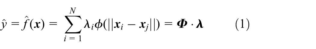
where N is the number of sampling points, x is the design variable vector, x _i is the ith sampling point, $| | x_{i} - x_{j} | |$ is the Euclidean norm, $ϕ$ is the kernel function, λ_i is the coefficient of the ith basis function, $Φ$ is $[ϕ_{1}, ϕ_{2}, \dots, ϕ_{N}]$ , $λ$ is ${[λ_{1}, λ_{2}, \dots, λ_{N}]}^{T}$ .

When x and ŷ in equation (1) are replaced with x _i and y _i, the N coefficients λ_i can be calculated using the following equations:

λ = A^{- 1} y

(2)

where A is the design matrix, $A_{ij} = ϕ (| | x_{i} - x_{j} | |)$ , $y = {[y_{1}, y_{2}, \dots, y_{N}]}^{T}$ .

Cubic, Linear, Gaussian, Multi-quadric, and other basis functions are often employed in RBF models. In order to improve computational efficiency, the most often used Linear to RBF function was employed as the basis function in the following study.

Because the RBF method works well for high-order nonlinear models but not well for linear models, a linear polynomial can be added to the model using the extended expression^19,20:

\begin{matrix} \hat{f} (x) = \sum_{i = 1}^{n} λ_{i} ϕ (‖ x - x_{i} ‖) + \sum_{j = 1}^{p} c_{j} g_{j} (x) \hat{f} (x) \\ = \sum_{i = 1}^{n} λ_{i} ϕ (‖ x - x_{i} ‖) + \sum_{j = 1}^{p} c_{j} g_{j} (x) \end{matrix}

(3)

\sum_{j = 1}^{n} λ_{i} g_{j} (x_{i}) = 0

(4)

where $g (x)$ is a linear polynomial, p is the number of items in the polynomial, c_j (j = 1, 2, 3, … , p) are the unknown coefficient, and λ_i (j = 1, 2, 3, … , p) are the coefficient. By combining equations (3) and (4), we can obtain (n + p) equations, which has the following matrix form:

(\begin{matrix} A & G \\ G^{T} & 0 \end{matrix}) (\begin{matrix} λ \\ c \end{matrix}) = (\begin{matrix} f \\ 0 \end{matrix})

(5)

where G_ij = g_j(x_i)(i = 1, 2, … , n, j = 1, 2, … , p), c = [c₁, c₂, … , c_p]^T, and the coefficients λ_i and c_i of the ERBF equation can be obtained by solving equation (5).

The adaptive metamodel-based global approximation method

This section goes into more detail on the proposed AMGA method. Section “Description of the AMGA method” discusses the reasoning and architecture of the new approach, and Section “Framework of the AMGA method” provides the method flow to further understand the AMGA method.

Description of the AMGA method

The design domain corner points and center points are sampled by the AMGA method to create an initial sample set S. The initial ERBF₁ model is built using the data set S in the initial design domain AREA₁, with the number of initial sample points N₀ = 2^d + 1, where d is the total number of design variables. The AMGA method then becomes an iterative loop:

In the first iteration, a design domain split point is obtained in the initial design domain AREA₁ using specific rules, and AREA₁ is split into two sub-domains AREA₂ and AREA₃ based on the splitting point, and AREA₂ and AREA₃ are then sampled using the design domain corner plus center points sampling method to obtain new sampling points. The ERBF₂ and ERBF₃ models are built on AREA₂ and AREA₃ utilizing the old and new sampling locations, respectively, and the ERBF₁ models are replaced by the ERBF₂ and ERBF₃ models. The AMGA method’s stopping condition is checked, and if it is not met, the second iteration is initiated. Determine which AREA₂ and AREA₃ sub-design domains should be further split. It is possible that only one sub-design domain needs to be further split (the source model lacks symmetry), or both sub-design domains (the source model has symmetry). If AREA₂ has to be split further, locate the splitting points inside the sub-design domain and split AREA₂ into two sub-design domains, AREA₂₁ and AREA₂₂. Sampling is carried out in AREA₂₁ and AREA₂₂ using the design domain corner plus center points sampling method to obtained extra sampling points to construct the ERBF₂₁ and ERBF₂₂ models, respectively, replacing the ERBF₂ model. The initial design domain AREA₁ is then split into three sub-domains, AREA₂₁, AREA₂₂, and AREA₃, and three metamodels, ERBF₂₁, ERBF₂₂, and ERBF₃ models, are constructed in these sub-design domains, respectively. The iterative procedure continues until the AMGA method’s stopping condition is met. Many metamodels are generated by the AMGA method’s continuous iterative computation. An ensemble, that is, RSS (response surface set), can represent these metamodels.

In the preceding process, the AMGA method involves two major problems: first, determining the best place to split the design domain, and second, determining which sub-design domains need to be further split. The AMGA method solves the first problem by combining the DIRECT²¹ algorithm with geometric techniques. Because DIRECT, as a heuristic direct search algorithm, is also a global optimization algorithm, the search criteria are as follows:

{\begin{matrix} find : x \\ max : K_{i} (x) \\ s . t . 1 \leq i \leq p \end{matrix} \cdot {L_{i}}^{p}

(6)

where x is a point in the design domain (the point can be imagined as a point on the metamodel surface), L_i is the edge length of the design domain along the ith dimension, p is the dimension of the design domain, i is 1, 2, … , p. K_i( x ) is the surface’s approximate curvature along the ith dimension at point x. The Hessian matrix from the ERBF model can be used to calculate K_i( x ); the bigger the value, the stronger the nonlinearity and the larger the curvature at this point. The precise calculation procedure for K_i( x ) is as follows:

The following is the ERBF model’s first order partial differential:

\frac{\partial \hat{f}}{\partial x} = \sum_{i = 1}^{N} \frac{λ_{i} ϕ' (r_{i})}{r_{i} (x)} {(x - x_{i})}^{T} + \sum_{j = 1}^{p} c_{j} g'_{j} (x)

(7)

where $r_{i} (x) = ‖ x - x_{i} ‖$ , $ϕ' (r_{i})$ is the first order partial differential of the radial basis function with respect to the relevant variable $r_{i}$ . For linear radial basis functions, $ϕ (r_{i}) = r_{i}$ , $ϕ' (r_{i}) = 1$ , $g'_{j} (x) = 1$ . Therefore, the final form of the Hessian matrix is calculated as follows:

H (x) = \frac{\partial^{2} \hat{f}}{\partial x^{2}} = \sum_{i = 1}^{N} \frac{λ_{i}}{r_{i} (x)} (Ø' (r_{i}) \cdot I + (Ø ″ (r_{i}) - \frac{Ø' (r_{i})}{r_{i} (x)})) (x - x_{i})^{T}

(8)

where I is the element matrix, $Ø ″ (r_{i})$ is the first-order partial differential $Ø' (r_{i})$ to r_i, and for linear radial basis functions, $Ø ″ (r_{i}) = 0$ . The Hessian matrix, according to the differential geometry principle, specifies the local curvature features, and the eigenvalues of the Hessian matrix can be used to determine the curvature at a location on the surface. The eigenvalues and eigenvectors of the Hessian matrix at a location on a surface correspond to that point’s primary curvature and direction. When we have p eigenvalues (k₁, k₂, … , k_p) and their eigenvectors (I₁, I₂, … , I _p) from the Hessian matrix, we can approximate the curvature value K_i(x) of a point on the surface in the ith dimension using the following equation:

{\begin{matrix} K_{i} (x) = | k_{m} \cdot \frac{I_{i}}{| I_{m} |} | \\ s . t . 1 \leq m \leq p \end{matrix}

(9)

Among them, m is 1, 2, … , p, I _m is the mth eigenvector, and I_i is the component of I _m in the ith dimension. Equation (9) gives the magnitude of the projection of the p eigenvalues in the ith dimension. If the metamodel is a hyperplane, the curvature will be zero, so a constraint needs to be added to the approximate curvature K_i(x).

K_{i} (x) \geq ε

(10)

If $K_{i} (x) \leq ε$ , then $K_{i} (x) = ε$ , and $ε$ is set to a very small number, which in this paper defaults to 10⁻⁸.

The following equation can be used to calculate the dimensional direction of the strongest nonlinearity and the corresponding position of the maximum curvature point, and the maximum curvature point is then used as the optimal splitting position of the design domain under the direction of the strongest nonlinearity:

j_{s} = \underset{1 \leq i \leq p}{\arg max} ({L_{i}}^{p} \cdot K_{p} (point))

(11)

The second problem is determining which sub-design domains need to be further split. The AMGA method presents a mechanism for assessing the accuracy of the metamodel. The ERBF model with the biggest error is chosen, and the corresponding sub-design domain is further split, based on the accuracy of the ERBF model constructed for each sub-design domain. In general, the greater the difference in source model values across sampling points, the stronger the model’s nonlinearity and the worse the model’s accuracy. As a result, the ERBF model’s accuracy can be measured directly by the difference between the maximum and minimum source model values between the sample points in the design domain. Equation (12) shows the specific rules.

T = h \cdot L_{1} \cdot L_{2} \cdot . . . \cdot L_{p}

(12)

Where, h represents the difference between the maximum and minimum source model values of the existing sampling points, L₁, L₂, … , L_p denotes the edge length of each dimension, and p represents the dimension of the problem, as shown in Figure 1 below.

Figure 1.

Calculation of h value on a one-dimensional curve.

Using the 2D source model as an example, the gray area in Figure 2(a) depicts the ERBF₁ model surface built from the initial design domain AREA₁. During the first iteration, the nonlinear intensity along dimensions 1 and 2 is searched on the ERBF₁ model surface using equation (11), and the maximum curvature points in two dimensional directions are obtained (e.g. the locations of the two black points a and b, where the direction of the arrow indicates the dimensional direction). If $K_{1} (a) \cdot {L_{1}}^{2}$ is greater than $K_{2} (b) \cdot {L_{2}}^{2}$ , it indicates that dimension 1 has more nonlinearity than dimension 2. As illustrated in Figure 2(b), the design domain AREA₁ is split into two sub-design domains AREA₂ and AREA₃ in the dimension 1 direction by point a. The design domain corner plus center points sampling method is used to sample in AREA₂ and AREA₃. The sampling points (the circle represents the sampling points obtained in the previous iteration, and the square represents the new sampling points obtained in this iteration) are utilized to construct the associated ERBF₂ and ERBF₃ models, and then the ERBF₁ model is replaced by the ERBF₂ and ERBF₃ models. If the stopping condition is not met, it begins the second iteration, as illustrated in Figure 2(c). Equation (12) is used to determine which sub-design domains require additional split. If AREA₃ has to be split further, use equation (11) to calculate the nonlinear strength of the ERBF₃ model in the dimension 1 and dimension 2 directions, and then split AREA₃ into sub-design domains AREA₃₁ and AREA₃₂ based on the maximum curvature point in that dimension. AREA₃₁ and AREA₃₂ are sampled using the design domain corner plus center points sampling method once more. The obtained sampled points are used to build the ERBF₃₁ and ERBF₃₂ models, and the ERBF₃ model is replaced by the ERBF₃₁ and ERBF₃₂ models. The iterative process is identical if a third iteration is necessary, as seen in Figure 2(d).

Figure 2.

The first three iterations of the splitting process of the design domain on a two-dimensional surface: (a) initial metamodel surface, (b) the first iteration, (c) the second iteration, and (d) the third iteration.

Following that, some special cases and parameter values are discussed. Due to the global search on the ERBF model surface when employing the AMGA method for adaptive design domain splitting and sampling, the DIRECT algorithm may encounter a circumstance where the maximum curvature point is very close to the design domain boundary. If the design domain split along this point, a very small and narrow part of the sub-design domain is formed. Because of this, the DIRECT algorithm may execute a local search within this sub-domain, resulting in a huge inaccuracy. To avoid this, provide a sufficient distance between the maximum curvature point and the design domain boundary.

Furthermore, the number of sub-design domains obtained by splitting the initial design domain with the AMGA method varies depending on the characteristics and parameter settings of the source model. If the source model is highly nonlinear, more sub-design domains are usually required to meet the approximate model’s accuracy criteria. As stopping conditions for iterative calculation, the AMGA method specifies three parameters, including the minimum edge length δ₁ of the sub-design domain, the error δ₂ of the ERBF model created from the sub-design domain, and the maximum number of iterations M.

If the initial design domain is large, δ₁ should be increased accordingly to avoid the initial design domain being over-split in the strongly nonlinear region and to enhance computing efficiency, but this will diminish the approximation model’s accuracy. Setting δ₂ to an acceptable value; however, too small δ₂ will over-split initial design domain, reducing computational efficiency but enhancing approximation model accuracy. The purpose of setting M is to limit the call to the source function for calculation. In summary, after selecting δ₁ and δ₂, M can be selected to balance the number of design domain splitting, computing efficiency, and approximation model accuracy.

Framework of the AMGA method

Figure 3 depicts the AMGA method’s flow chart.

Input: Stopping conditions.

(1) Minimum sub-design domain edge length δ₁;

(2) Single approximation model error δ₂;

(3) Maximum number of iterations M (Optional).

Output: the RSS model.

Step 1. Generating initial data points using the design domain corner plus center points sampling method;

Step 2. Calculate the source model values for each sampled point and store the data in the S set;

Step 3. Construct the initial ERBF model using data set S.

Step 4. Repeat Steps 4(a)–(d) until the stopping condition is met.

(a) Determine whether or not the iteration meets the exit stopping condition.

(b) Use equation (12) to determine which design domain of the ERBF model in the RSS needs to be further split;

(c) New sampling points are obtained by adaptive splitting of the design domains using equation (11), and new ERBF models are constructed in the sub-design domains;

(d) Add the new ERBF models to the RSS, reorder all ERBF models, and repeat step (a).

Step 5. Export the RSS.

Figure 3.

Flowchart of the adaptive metamodel-based global approximation (AMGA) method.

Test of the adaptive metamodel-based global approximation method

Experimental setup

All tests were run in Matlab™ 2022a on a computer with 64 GB of RAM and an Intel i7-12700k 3.6GHz processor. To speed up the creation of the ERBF model, linear basis functions were used as kernel functions in this research.

Numerical tests

The effect of global approximation and design domain splitting for 2D test functions

Six common functions are tested in this part to demonstrate the approximate processing effect of the AMGA method for diverse source functions, the splitting of the design domain, and the distribution of sample points. These functions’ nonlinear strength varies. The basic forms of the six functions studied are depicted in Figure 4. Simple Exponential, Chichinadze, and Himmelblau are simple two-dimensional functions with weak nonlinearity and relatively flat function values. In comparison, the nonlinearities of Easom, Peak, and Trefethen4 are stronger, with Trefethen4 having several peaks and valleys and Easom having a valley with a high verticality.

Figure 4.

Test function surface plots: (a) simple exponential function, (b) Chichinadze function, (c) Himmelblau function, (d) Easom function, (e) Peak function, and (f) Trefethen4 function.

The design domain splitting of the six test functions is shown in Figure 5, with the black dots “•” indicating the 100 sampling points created when the test functions are approximated using the AMGA method. When dealing with test functions of varying nonlinear strength, the AMGA method can adaptively split the design domain, as shown in Figure 5(a) to (f). Furthermore, if the test function exhibits strong nonlinearity in some regions, the more the design domain is split in that region, the more intense the sampling points are; conversely, if the test function exhibits weak nonlinearity in some regions, the less the design domain is split in that region, the fewer the sampling points are.

Figure 5.

Test model design domain splitting: (a) simple exponential function, (b) Chichinadze function, (c) Himmelblau function, (d) Easom function, (e) Peak function, and (f)Trefethen4 function.

Figure 6 depicts the approximation model shapes constructed with the AMGA method, which are very similar to the shapes of the test functions in Figure 4.

Figure 6.

The shapes of the approximate models: (a) simple exponential function, (b) Chichinadze function, (c) Himmelblau function, (d) Easom function, (e) Peak function, and (f)Trefethen4 function.

Comparison with different methods

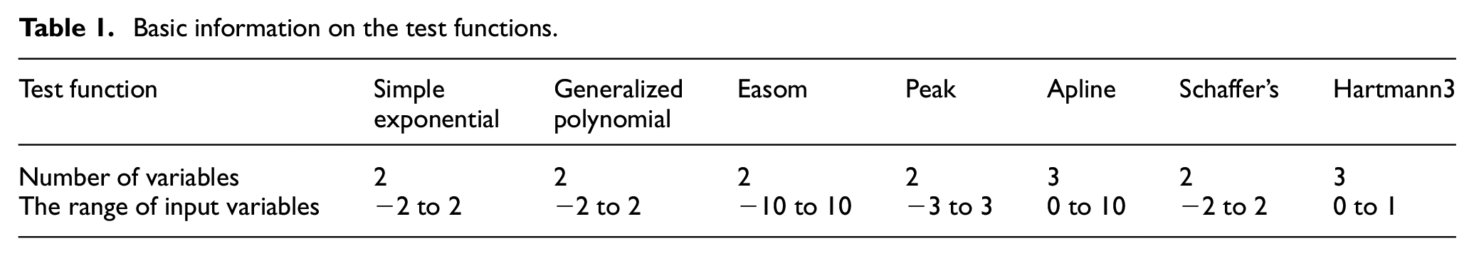
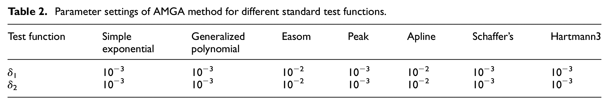
To evaluate the precision and effectiveness of the AMGA method, seven typical functions are used in this section. Two additional sampling methods are used in addition to the AMGA method to compare with it. The first is the roughness-based adaptive sampling (ASRS) method, which enables adaptive domain splitting to obtain additional sampling points and creates a full quadratic polynomial model using the sampling points nearby the input point. The second method, known as Latin Hypercube Sampling (LHS), directly builds the metamodel using the sampled points. The necessary information regarding typical test functions are listed in Table 1. The parameter settings for the AMGA method are listed in Table 2. To lessen the impact of random errors during testing, 100 trials are conducted for each function. For each approach, the root mean square error and the total number of source model calls are listed in Tables 3 to 6.

Table 1.

Basic information on the test functions.

Test function	Simple exponential	Generalized polynomial	Easom	Peak	Apline	Schaffer’s	Hartmann3
Number of variables	2	2	2	2	3	2	3
The range of input variables	−2 to 2	−2 to 2	−10 to 10	−3 to 3	0 to 10	−2 to 2	0 to 1

Table 2.

Parameter settings of AMGA method for different standard test functions.

Test function	Simple exponential	Generalized polynomial	Easom	Peak	Apline	Schaffer’s	Hartmann3
δ ₁	10⁻³	10⁻³	10⁻²	10⁻³	10⁻²	10⁻³	10⁻³
δ ₂	10⁻³	10⁻³	10⁻²	10⁻³	10⁻²	10⁻³	10⁻³

Table 3.

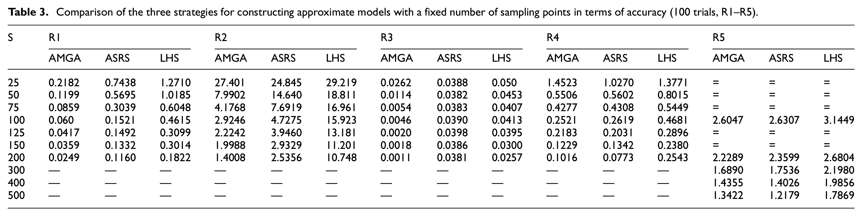
Comparison of the three strategies for constructing approximate models with a fixed number of sampling points in terms of accuracy (100 trials, R1–R5).

S	R1			R2			R3			R4			R5
S	AMGA	ASRS	LHS	AMGA	ASRS	LHS	AMGA	ASRS	LHS	AMGA	ASRS	LHS	AMGA	ASRS	LHS
25	0.2182	0.7438	1.2710	27.401	24.845	29.219	0.0262	0.0388	0.050	1.4523	1.0270	1.3771	=	=	=
50	0.1199	0.5695	1.0185	7.9902	14.640	18.811	0.0114	0.0382	0.0453	0.5506	0.5602	0.8015	=	=	=
75	0.0859	0.3039	0.6048	4.1768	7.6919	16.961	0.0054	0.0383	0.0407	0.4277	0.4308	0.5449	=	=	=
100	0.060	0.1521	0.4615	2.9246	4.7275	15.923	0.0046	0.0390	0.0413	0.2521	0.2619	0.4681	2.6047	2.6307	3.1449
125	0.0417	0.1492	0.3099	2.2242	3.9460	13.181	0.0020	0.0398	0.0395	0.2183	0.2031	0.2896	=	=	=
150	0.0359	0.1332	0.3014	1.9988	2.9329	11.201	0.0018	0.0386	0.0300	0.1229	0.1342	0.2380	=	=	=
200	0.0249	0.1160	0.1822	1.4008	2.5356	10.748	0.0011	0.0381	0.0257	0.1016	0.0773	0.2543	2.2289	2.3599	2.6804
300	—	—	—	—	—	—	—	—	—	—	—	—	1.6890	1.7536	2.1980
400	—	—	—	—	—	—	—	—	—	—	—	—	1.4355	1.4026	1.9856
500	—	—	—	—	—	—	—	—	—	—	—	—	1.3422	1.2179	1.7869

Table 4.

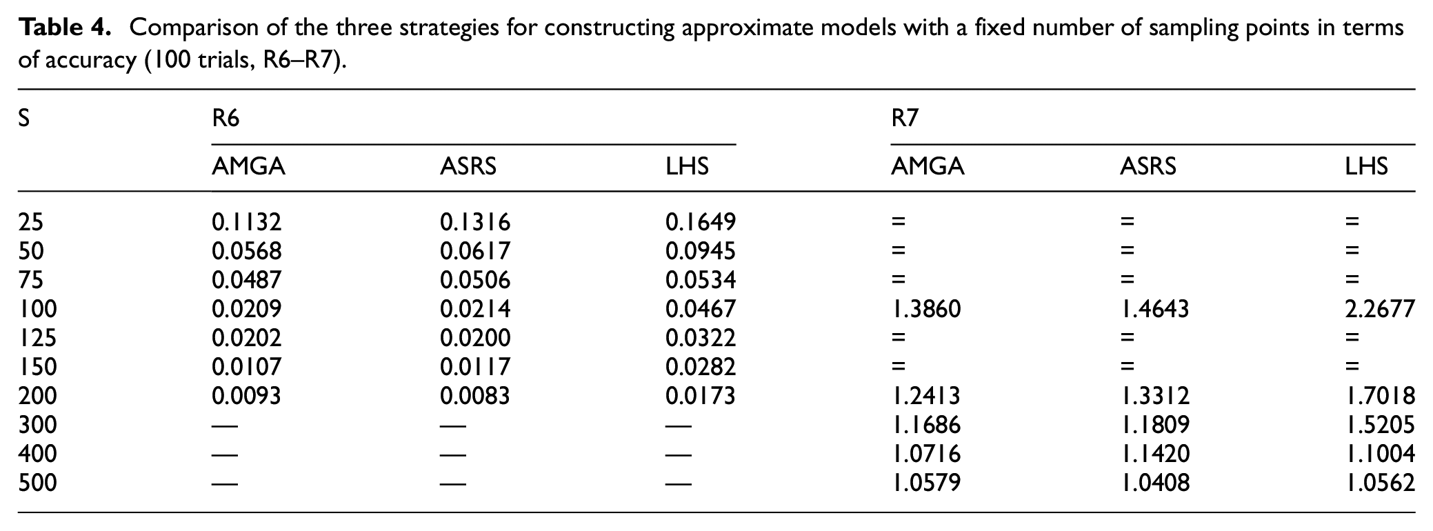
Comparison of the three strategies for constructing approximate models with a fixed number of sampling points in terms of accuracy (100 trials, R6–R7).

S	R6			R7
S	AMGA	ASRS	LHS	AMGA	ASRS	LHS
25	0.1132	0.1316	0.1649	=	=	=
50	0.0568	0.0617	0.0945	=	=	=
75	0.0487	0.0506	0.0534	=	=	=
100	0.0209	0.0214	0.0467	1.3860	1.4643	2.2677
125	0.0202	0.0200	0.0322	=	=	=
150	0.0107	0.0117	0.0282	=	=	=
200	0.0093	0.0083	0.0173	1.2413	1.3312	1.7018
300	—	—	—	1.1686	1.1809	1.5205
400	—	—	—	1.0716	1.1420	1.1004
500	—	—	—	1.0579	1.0408	1.0562

Table 5.

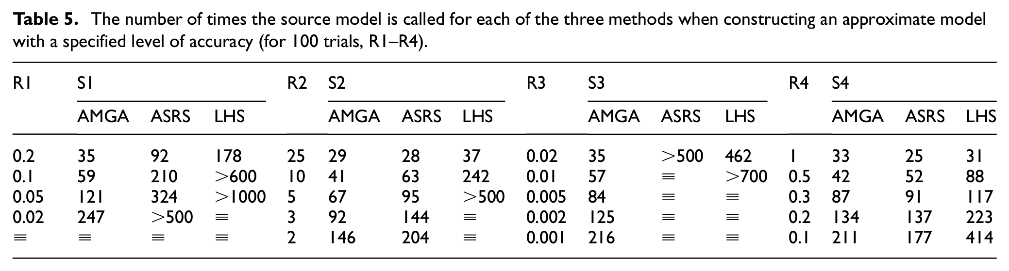
The number of times the source model is called for each of the three methods when constructing an approximate model with a specified level of accuracy (for 100 trials, R1–R4).

R1	S1			R2	S2			R3	S3			R4	S4
R1	AMGA	ASRS	LHS	R2	AMGA	ASRS	LHS	R3	AMGA	ASRS	LHS	R4	AMGA	ASRS	LHS
0.2	35	92	178	25	29	28	37	0.02	35	>500	462	1	33	25	31
0.1	59	210	>600	10	41	63	242	0.01	57	≡	>700	0.5	42	52	88
0.05	121	324	>1000	5	67	95	>500	0.005	84	≡	≡	0.3	87	91	117
0.02	247	>500	≡	3	92	144	≡	0.002	125	≡	≡	0.2	134	137	223
≡	≡	≡	≡	2	146	204	≡	0.001	216	≡	≡	0.1	211	177	414

Table 6.

The number of times the source model is called for each of the three methods when constructing an approximate model with a specified level of accuracy (for 100 trials, R5–R7).

R5	S5			R6	S6			R7	S7
R5	AMGA	ASRS	LHS	R6	AMGA	ASRS	LHS	R7	AMGA	ASRS	LHS
2.5	116	122	239	0.1	28	33	46	1.3	85	94	314
2	235	242	387	0.05	53	80	71	1.2	164	271	384
1.5	356	378	>600	0.03	91	93	137	1.1	372	445	398
1.3	579	462	≡	0.02	128	125	169	1.0	569	543	>600
1.2	>800	512	≡	0.01	192	158	349	0.9	728	>800	≡

Tables 3 to 6 illustrate the test results of constructing the approximation model using the three sampling methods. S, S1–S7 represent the number of sample points, which corresponds to the number of calls to the source function for calculation. R1–R7 is the root mean square error of constructing the approximation model, which reflects the approximation model’s correctness. In Tables 5 and 6, the more calls to the source model necessary for the same root mean square error, the longer the time required, and the less efficient the associated sampling approach. The symbol “—” in the table indicates that there is no change in the trend of the subsequent test results and is omitted; the symbol “=” indicates that there are fewer sampling points and is not taken into account; and the symbol “≡” indicates that there are too many calls to the source function and is not taken into account.

The test results in Tables 3 to 6 demonstrate that the AMGA method outperforms the ASRS and LHS methods for the simple exponential, generalized polynomial, and Easom functions. It rivals the ASRS method on Peak, Apline, Schaffer’s, and Hartmann3 functions.

For the simple exponential function, Table 3 indicates that the AMGA method outperforms the ASRS and LHS methods, allowing a more accurate approximation model to be constructed from the start with fewer sampling points. Table 5 shows that the AMGA method, when compared to the other two methods, can construct an approximation model with some accuracy while using fewer source function calls. The findings in Tables 3 to 6 indicate the efficiency of the AMGA approach for the generalized polynomial and Easom functions.

For the Peak and Schaffer functions, the statistics in Tables 3 to 6 show that the AMGA and ASRS approaches have their own advantages and weaknesses, although both are much better than the LHS method.

For the Apline and Hartmann3 functions, the data in Tables 3 and 4 show that the AMGA method initially constructs a more accurate approximation model than the other two methods. As the number of sample points increases, the accuracy of the approximation model constructed by the AMGA method is slightly lower than that of the ASRS method, but better than that of the LHS method. Tables 5 and 6 indicates that the AMGA method initially produces a high-accuracy approximate model with the fewest source function calls. In terms of the number of source function calls, the AMGA approach is comparable to the ASRS method as accuracy rises.

Engineering cases

Problem description

As shown in Figure 7, the components of the electric vehicle (EV) simulation model are estimated using the AMGA method. The EV simulation model is mainly consists of drive, controller, and vehicle body components. While the vehicle body components include models of the motor, powertrain, battery, and transmission system, etc. The EV simulation model is primarily used for powertrain matching analysis, control and diagnostic algorithm development, and hardware-in-the-loop (HIL) testing, which necessitates a real-time EV model. The vehicle body, on the other hand, has the highest computational complexity, which has a direct impact on the overall computational complexity of the model. A metamodel is employed for simulation instead of the body components to speed up the calculation of the EV model and ensure real-time performance.

Figure 7.

Electric vehicle model.

The NEDC^22,23 cycle condition is used as the drive cycle of the car on the road in the EV simulation model. As indicated in Figure 8, the NEDC is made up of four cycles: the urban drive cycle condition (ECE-15) and the extra-urban drive condition (EUDC). To simplify the calculation, ECE-15 is chosen as the simulation drive.

Figure 8.

NEDC driving cycle.

Process of model approximation

A model processing method based on feedback with fixed step size is provided to achieve the approximation of the car body of the EV simulation model. Generally, three states exist during simulation model operation: the previous simulation model state, the current simulation model state, and the latter simulation model state, as shown in the Figure 9 below.

Figure 9.

The three states of the model.

Where In_p is the pth input to the model and Out_K is the Kth output of the model. The model states before and after are ignored, and the current state is treated as follows.

Step 1: Create the Independent Simulation Module (ISM).

(1) Add input and output ports to the ISM, including state variable input and output ports.

(2) Using historical simulation data for the entire EV model, generate a range of values for the ISM input variables.

(3) Calculate the time step t₀. At different simulation times t₀, the ISM will produce varied outcomes. t₀ is set to 0.1 s to allow the ISM to run in real-time later on. The processed ISM, as illustrated in Figure 10, contains the input and output ports, as well as the state variables and t₀, and the ISM can be represented by the following equation.

\begin{matrix} {Ou t_{1}, Ou t_{2}, . . ., Ou t_{K}, S_{1}^{'}, S_{2}^{'}, . . ., S_{M}^{'}} = \\ ISM_t_{0} {I n_{1}, I n_{2}, . . ., I n_{P}, S_{1}, S_{2}, . . ., S_{M}} \end{matrix}

(13)

Figure 10.

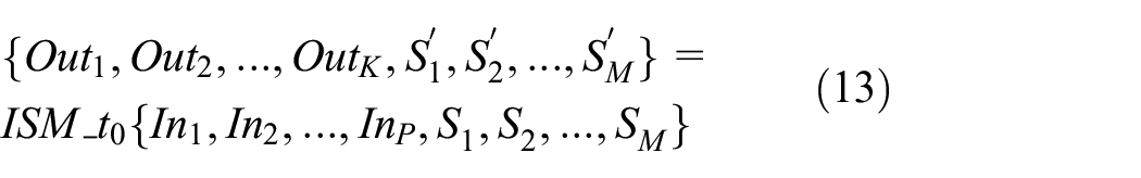
ISM of the simulation model.

Where S_M is the Mth input of the state variable, S_M’ is the Mth output of the state variable, ISM represents an independent simulation module based on t₀.

Step 2: The ISM is approximated using the AMGA method.

Step 3: Confirm the approximation model’s accuracy, which can be measured using R², as stated in the following equation.

R^{2} = 1 - \frac{\sum_{k = 1}^{n} {(f (x^{k}) - f_{approximate} (x^{k}))}^{2}}{\sum_{k = 1}^{n} {(f (x^{k}) - {\bar{f}}_{approximate})}^{2}}

(14)

Where f( x ^k) represents the true value of point x^k on the source model, f_approximate( x ^k) represents the valuation of point x ^k on the approximation model, and ${\bar{f}}_{approximate}$ is the average of the evaluations of all test points on the approximate mode. R² is a value between 0 and 1 that represents the approximation model’s correctness; the closer R² is to 1, the more accurate the approximation model is. The components of the source model, on the other hand, can be replaced by the approximation model. The modified simulation model containing the approximation model components is simulated and compared to the source model. If the modified approximation model’s accuracy meets the requirements, the current state’s processing is finished.

Step 4: If the approximation model’s accuracy does not meet the requirements, return to step (2) and continue processing the ISM using AMGA method to further improve the accuracy of the approximation model.

In addition, for the state variables in the simulation model, the specific form is as follows.

{\begin{matrix} f (u, s, s', t) = 0 \\ y = g (s, s', u, t) \end{matrix}

(15)

where t, u , s , and y are the time, input, state variables, and output, respectively.

To validate the approximation model’s accuracy, the M state variables (S₁, S₂, … , S_M) are processed so that they are self-looping and can be automatically updated during the simulation, as illustrated in Figure 11. The ISM’s input port is P inputs plus M state variable inputs, and its output port is P outputs plus M state variable outputs. The output of the state variable differs from the input by a time step delay of t₀.

Figure 11.

State variable processing.

Approximation model test

Create the ISM of the car body model, add three input ports (acceleration command M_cmd, brake command B_cmd, current battery state S_OC). Add two output ports (motor rotation angular velocity W, discharge state S_OCn for the next time step) with a time step delay t₀ of 0.1 s (Figure 12).

Figure 12.

ISM of the vehicle body model.

The AMGA method was utilized to construct a three-input, one-output approximation model for W and S_OCn, respectively, once the ISM of the car body model was established. The approximation process’s parameters are set to M_cmd∈[0,1], B_cmd∈[0,1], S_OC∈[93,100], δ₁ = 10⁻¹, δ₂= 10⁻³.

As illustrated in Figure 13, the procedure of substituting the approximation component for the matching vehicle body component in the original EV simulation model is as follows:

In the Matlab environment, obtain the approximation model’s relevant data: the approximate model’s coefficient column vectors and the sampling point matrix.

Using the From Workspace module, import the approximation model-related data and the input data into the Simulink environment.

Create a data bus in the Simulink environment so that data is transported in the Simulink model via a data bus.

Create a function module and a function valuation module in the Simulink environment. The former collects the data imported in step (2) and provides it as a structure to the following function valuation module; the latter analyzes the structure and uses the input data to perform valuation.

In the Simulink model, the input and output of the state variables are connected first and last, and the fixed-step delay module Memory is added between the input and output connections of the state variables.

Encapsulate the Simulink model and replace the ISM.

Figure 13.

Verify the accuracy of the approximation component on the electric vehicle.

The simulation results of modified EV simulation model using the approximation component were compared to the original EV simulation model results, as shown in Figure 14.

Figure 14.

Comparison of simulation results between EV simulation model with approximate component and original EV simulation model.

The variable curves obtained from the modified EV simulation model with the approximation component are essentially the same as the original EV simulation model, as shown in the Figure 14. The R² values of SOC and W obtained by the AMGA method for the modified EV simulation model are 0.8758 and 0.8672, while the R² values of SOC and W obtained by the ASRS method are 0.9053 and 0.8601. As a result, the R² values obtained by both the AMGA method and the ASRS method are very close to each other and both are close to 1, which indicates that the modified electric vehicle simulation model has good accuracy. The original EV simulation model’s computation time, on the other hand, differs from that of the modified EV simulation model. The former takes roughly 15 min, whereas the latter takes about 1 min. As a result, the modified EV simulation model is significantly more computationally efficient than the original.

The approximation model can then be constructed by code and imported into the target machine, where a physical controller can be used to operate the running approximation model, enabling a semi-physical simulation experiment (Hardware-in-loop, HIL).

Conclusions

To overcome the black-box model approximation problem in large design domains, this work proposes a global approximation method AMGA based on adaptive metamodels. The method incorporates the following innovations: first, it use the Hessian matrix to determine the surface curvature of the metamodel in a given dimension; second, it employs the DIRECT method in conjunction with the Hessian matrix to determine the maximum curvature point of the metamodel surface; third, the design domain is split using the maximum curvature point to generate more sampling points; fourth, the method adds a novel mechanism for judging metamodel accuracy. The proposed method can split the large design domain continuously and construct new metamodel in the sub-design domain, avoiding the construction of a single, simple approximate model in the large design domain. This substantially enhances the overall approximation accuracy of these large design domain models and avoids the approximation model generation being slowed or even failing due to over-sampling inside the design domain.

This method, however, has several drawbacks. First, the AMGA method calculates surface curvature from a geometric standpoint, and the geometric method has its own disadvantages. As a result, it does not handle problems with more than four dimensions well, and more research is required to solve such difficulties; second, even if the design domain corners sampling points are continuous, the continuity problem of sub-domain boundaries after design domain splitting cannot be handled, and the continuity of all boundaries cannot be guaranteed; third, using the AMGA method to construct approximation models of many objectives at the same time is a difficulty that need to be addressed; fourth, the AMGA method has limited approximation power when dealing with the constraint function problem, and the constructed approximation model has poor accuracy. This problem can be used as a follow-up research point to enable the AMGA method to handle constraint functions with high accuracy and to research the approximation problem of constraint functions in discontinuous regions further.

Footnotes

Handling Editor: Chenhui Liang

Declaration of conflicting interests

The author(s) declared no potential conflicts of interest with respect to the research, authorship, and/or publication of this article.

Funding

The author(s) disclosed receipt of the following financial support for the research, authorship, and/or publication of this article: This work is supported by the Commonweal Projects of Zhejiang Province of China (number GF20E090020).

ORCID iD

Yin Xiao-liang

References

Soares do Amaral

Montevechi

JAB

Miranda

RDC

, et al. Metamodel-based simulation optimization: a systematic literature review. Simul Model Pract Theory 2022; 114: 102403.

Ripp

. Application of the metamodel. In: Ripp

(ed.) A metamodel for heritage-based urban development. Heritage studies. Berlin: Springer, 2022, pp.163–172.

. A novel single-loop meta-model importance sampling with adaptive Kriging for time-dependent failure probability function. Struct Multidiscipl Optim 2023; 66: 79.

Liu

Ong

Cai

. A survey of adaptive sampling for global metamodeling in support of simulation-based complex engineering design. Struct Multidiscipl Optim 2018; 57: 393–416.

Lin

. An efficient robust concept exploration method and sequential exploratory experimental design. PhD Dissertation, Georgia Institute of Technology, USA, 2004.

Steiner

Bourinet

Lahmer

. An adaptive sampling method for global sensitivity analysis based on leastsquares support vector regression. Reliab Eng Syst Saf 2019; 183: 323–340.

Wang

. Adaptive response surface method using inherited Latin hypercube design points. J Mech Des 2003; 125: 210–220.

Wei

Chen

. Global optimization method based on incremental radial basis functions. Appl Mech Mater 2012; 121–126: 3950–3954.

Zhong

Kealy

Duckham

. Stream Kriging: incremental and recursive ordinary Kriging over spatiotemporal data streams. Comput Geosci 2016; 90: 134–143.

10.

Laskov

Genl

Krüger

, et al. Incremental support vector learning, analysis, implementation and applications. J Mach Learn Res 2006; 7: 1909–1936.

11.

Parnianifard

Chancharoen

Phanomchoeng

, et al. A new approach for low-dimensional constrained engineering design optimization using design and analysis of simulation experiments. Int J Comput Intell Syst 2020; 13: 1663–1678.

12.

Parnianifard

Zemouche

Chancharoen

, et al. Robust optimal design of FOPID controller for five bar linkage robot in a cyber-physical system: a new simulation-optimization approach. PLoS One 2020; 15: e0242613.

13.

Shahsavani

Grimvall

. An adaptive design and interpolation technique for extracting highly nonlinear response surfaces from deterministic models. Reliab Eng Syst Saf 2009; 94: 1173–1182.

14.

Myers

Montgomery

. Response surface methodology: process and product optimization using designed experiments. Toronto, ON: John Wiley and Sons, Inc, 2002.

15.

Kleijnen

JPC

. Kriging metamodeling in simulation: a review. CentER Discussion Paper, 13, Tilburg University, 2007.

16.

Buhmann

. Radial basis functions. Cambridge: Cambridge University Press, 2006.

17.

Clarke

Griebsch

Simpson

. Analysis of support vector regression for approximation of complex engineering analyses. J Mech Des 2005; 127: 1077–1087.

18.

Parnianifard

Azfanizam

Ariffin

MKA

, et al. Comparative study of metamodeling and sampling design for expensive and semi-expensive simulation models under uncertainty. Simulation 2020; 96(1): 89–110.

19.

Krishnamurthy

. Response surface approximation with augmented and compactly supported radial basis functions. In: Proceedings of the 44th AIAA/ASME/ASCE/AHS/ASC structures, structural dynamics, and materials conference, Norfolk, VA, USA, 7–10 April 2003.

20.

Fang

Horstemeyer

. Global response approximation with radial basis functions. Eng Optim 2006; 38: 407–424.

21.

Jones

. Direct global optimization algorithm. In: Floudas

Pardalos

(eds) Encyclopedia of optimization. Boston, MA: Springer, 2001, pp.431–440.

22.

GB/T 18385-2005. Electric vehicles-power performance-test method (ISO 8715; 2001 electric road vehicles-road operating characteristics).

23.

GB/T 18386-2005. Electric vehicles-energy consumption and range-test procedures.

An adaptive metamodel-based global approximation method for black-box type problems

Abstract

Keywords

Introduction

Metamodelling technique

The adaptive metamodel-based global approximation method

Description of the AMGA method

Framework of the AMGA method

Test of the adaptive metamodel-based global approximation method

Experimental setup

Numerical tests

The effect of global approximation and design domain splitting for 2D test functions

Comparison with different methods

Engineering cases

Problem description

Process of model approximation

Approximation model test

Conclusions

Footnotes

Declaration of conflicting interests

Funding

ORCID iD

References