Sage Journals: Discover world-class research

Abstract

In this paper, in order to solve the problem that it is difficult to carry out accurate fault diagnosis for gearbox under noise environment, complete ensemble imperial mode decomposition with adaptive noise analysis (CEEMDAN) is used to solve the sample entropy of the original signal and each intrinsic mode function (IMF) component, adaptive wavelet is adopted to decompose and reconstruct IMF with large sample entropy for noise reduction, and first layer wide convolution kernel deep convolution neural network (WDCNN) and long short term memory (LSTM) are used to extract the basic digital features of the reconstructed signal and the correlation features between the features. Therefore, a new fault diagnosis method for gearbox under noise environment is proposed. Taking the public data set of Jiangsu Qiangpeng Diagnostic Engineering Co., Ltd as the research object, the experiments were carried out with the method proposed in this paper. The experimental results show that the proposed method has high accuracy and strong anti-noise ability. Under the environment of no noise and low noise, the fault diagnosis accuracy of the gearbox is 100%; even if the signal to noise ratio is −4 dB, the fault diagnosis accuracy of the gearbox can still reach 99.97%. Therefore, this paper provides a method support for gearbox fault diagnosis under noise environment.

Keywords

Adaptive wavelet CEEMDAN WDCNN LSTM gearbox fault diagnosis

Introduction

Gearbox is an important deceleration and reversing device in construction machinery, mining machinery and transportation equipment. The safety and stability of gearbox is the primary premise to ensure the continuous production of all kinds of machinery. During the use of gearbox, the pitting corrosion, wear, tooth breakage and other phenomena between gears are often caused by pulsating impact load, oxidation corrosion and continuous high-intensity work, which lead to mechanical shutdown and even major safety accidents. Therefore, it is necessary to take reasonable means to monitor the gearbox and timely repair when similar faults occur, so as to achieve the purpose of prevention and diagnosis of gearbox fault.

With the continuous development of whole world economy, all kinds of production machinery are widely used in various field, so many scholars focus on the fault diagnosis research of gearbox. The traditional fault diagnosis methods include Fourier transform,¹ wavelet transform,² empirical mode decomposition (EMD)³ and other signal processing methods.^4,5 Many scholars could separate the noise from the signal to a certain extent when they used the traditional methods to diagnose gearbox fault. However, when faced with the influence of many factors such as multiple fault types, large amount of data, and wide range of noise, the traditional fault diagnosis methods can not accurately diagnose gearbox fault due to simple feature extraction and inaccurate classification results. The emergence of deep learning theory provides an invisible and adaptive feature extraction and classification method for many scholars. With the development of deep learning theory, various deep learning based network models have been used in image recognition,^6,7 machine vision,^8,9 object detection,^10,11 natural language processing^12,13 and other fields. Among them, Visual geometry group (VGG) has the ability of multi-scale feature extraction,¹⁴ which has high accuracy for image recognition; One-dimensional convolution neural network has a large receptive field of vision and less parameters, and it has the characteristics of fast training speed and ultra-high accuracy in vibration signal recognition¹⁵; general adverse network (GAN) can generate samples according to the characteristics of source domain samples, which solves the problem of unbalanced data samples.¹⁶

Health monitoring and fault diagnosis of rotating machinery has always been a hot research topic in the field of mechanical engineering, and bearing and gearbox are typical rotating machinery. Therefore, fault diagnosis of bearing and gearbox based on deep learning theory has been widely studied and applied. In the research of bearing fault diagnosis, in order to solve the problem of how to effectively mine features from big data and use new advanced methods to accurately identify bearing health. He and He proposed a bearing fault diagnosis method based on deep learning on the basis of short-time Fourier transform.¹⁷ Chen et al. proposed a fault diagnosis method based on cyclic spectral coherence and convolutional neural network, which embedded domain diagnosis knowledge into deep learning to obtain appropriate features related to good health, thus improving the recognition performance of rolling bearing fault.¹⁸ In order to overcome the shortcomings of bearing fault diagnosis based on vibration signal, Hoang and Kang proposed a bearing fault diagnosis method based on motor current signal by using deep learning and information fusion.¹⁹ Nguyen et al. transformed the measured vibration signal into a new data form of multi domain image representation, and proposed a bearing fault diagnosis method based on deep neural network.²⁰ In terms of fault diagnosis research of gearbox, in order to make up for the shortcomings of limited sample data, Saufi et al. designed a deep neural network model based on stacked sparse automatic encoder, and successfully applied it to the accurate fault diagnosis of gearbox.²¹ Based on the advantage that deep learning can automatically learn high-dimensional features from the original measured data, Singh et al. proposed a new domain adaptive gearbox fault diagnosis method based on deep learning.²² Based on the vibration data of aircraft gearbox in time domain and frequency domain, Mallikarjuna et al. proposed two deep learning models to realize fault diagnosis of gearbox.²³ Based on the data of wind farm monitoring and data, Yang and Zhang proposed a gearbox fault monitoring method by using a deep joint variational automatic encoder.²⁴

Although one-dimensional convolution neural network has powerful and invisible feature extraction ability, convolution neural network uses convolution kernel sliding method to extract feature information from vibration data, thus splitting the correlation information of feature changes before and after vibration signal. When the vibration signals contain noise, the fault signal samples will have similar characteristics; at this time, it is difficult for the convolutional neural network to effectively classify faults, which leads to failure of fault diagnosis. Therefore, in this paper, a noise reduction method was proposed to filter the noise in the vibration signal and preprocess the vibration data. The basic principle of this noise reduction method is as follows. Firstly, the sample entropy (S) of the vibration signal without noise is obtained,²⁵ then complete ensemble imperial mode decomposition with adaptive noise analysis (CEEMDAN) is used to perform adaptive mode decomposition for the vibration signal with mixed noise²⁶ to obtain the component sample entropy (SampEN) step by step, and finally adaptive wavelet de-noising is applied to the intrinsic mode functions (IMF) whose sample entropy is greater than S, and each IMF after de-noising is weighted and reorganized. In addition, a method of feature extraction and classification of vibration data after noise reduction was proposed based on first layer wide convolution kernel deep convolution neural network (WDCNN)²⁷ and long short term memory (LSTM).²⁸ The fault diagnosis experiments of gearbox were carried out, and the experimental results show that the fault diagnosis accuracy of the gearbox is 100% under the environment of no noise and low noise; even if the signal to noise ratio is −4 dB, the fault diagnosis accuracy of the gearbox can still reach 99.97%, which verify the effectiveness of the method proposed in this paper and provide a method reference for the fault diagnosis of gearbox. The contribution and innovation of this paper is to propose a new fault diagnosis method for gearbox in noisy environment by combining CEEMDAN, wavelet analysis and convolution neural network, which solves the problem of accurate fault diagnosis for gearbox in strong noise environment.

The rest of this paper is arranged as follows. The experimental equipment and data of gearbox fault diagnosis are introduced in Section 2. Section 3 gives the method and process of gearbox fault diagnosis. The training accuracy and visualization results of the proposed neural network model are obtained in Section 4. Section 5 presents the results of gearbox fault diagnosis by using the method proposed in this paper under different noise environments and the experimental comparison results with other methods. Some conclusions of this paper are drawn in Section 6.

Experimental data

The experimental data in this paper was taken from the public data set of the fault diagnosis experimental platform of Jiangsu Qianpeng Diagnostic Engineering Co., Ltd. The calibration speed of the motor used in this paper is 1000 rad/min, and the measured speed is 880 rad/min. There are two standard spur gears with 35 teeth, two modules and pressure angle of 20° inside the gearbox. The vibration data was measured at the motor side bearing, gearbox input and output side bearing, load output side bearing, and these vibration data simulated four output conditions with load current of 0, 0.05, 0.1 and 0.2 A, respectively. In this paper, the vibration data of the load bearing of the input shaft was taken as the sample data for the fault diagnosis of the gearbox. The experimental equipment is shown in Figure 1.

Figure 1.

Experimental equipment.

In Figure 1, A represents the motor side bearing of the input shaft; B represents the input side bearing of the gearbox; C represents output side bearing of the gearbox; D represents the load output side bearing of the output shaft. In the experiment, the tooth root and the meshing point are the most stressed parts of the two gears in the meshing process. Therefore, this paper mainly conducted diagnosis research on the five most common gear faults, namely, pitting corrosion, wear, tooth breakage, pitting corrosion and wear, tooth breakage and wear. Each fault data was measured by an acceleration sensor, and the data length is 53248.

Fault diagnosis process

After obtaining five different kinds of fault vibration data from the experimental equipment, the vibration data was sampled repeatedly to achieve the purpose of data enhancement. In addition, Gaussian noises with different signal-to-noise ratio were added to the vibration data to simulate the different noise conditions in the use environment. The adaptive empirical mode decomposition method was used to decompose the vibration signal with noise, and the sample entropy of each IMF after decomposition was calculated, as well as the sample entropy of the vibration signal without noise and mode decomposition. Through the comparison of sample entropy, IMF components that need wavelet de-noising were selected. After wavelet de-noising, all IMF components were added and recombined to achieve the purpose of de-noising. The fault diagnosis process is shown in Figure 2.

Figure 2.

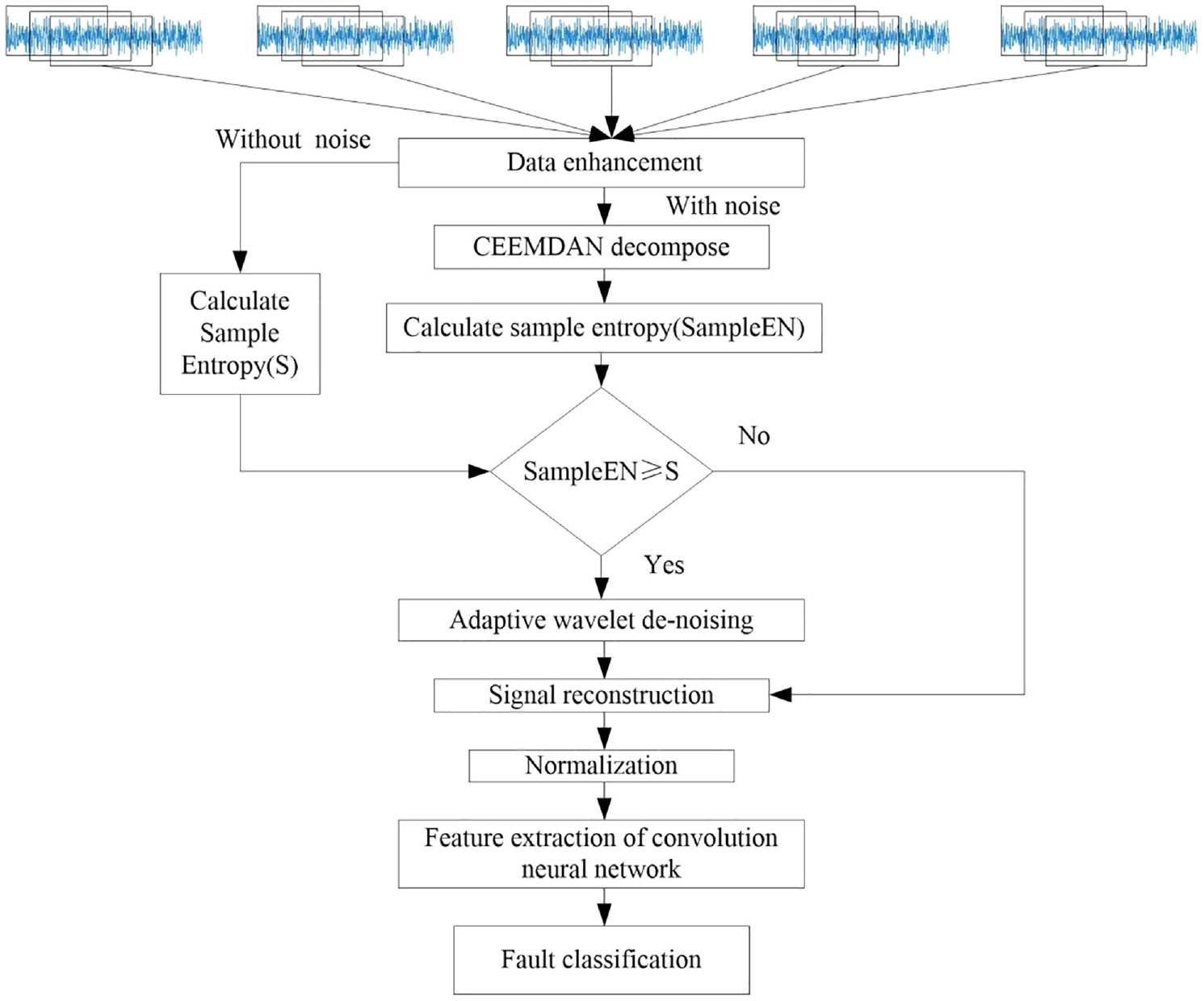
Fault diagnosis process.

Data preprocessing

Because there are only 53,248 points of each kind of fault data collected in the experiment, enough data samples can’t be cut out in one direction to train the neural network. Therefore, the sliding window method was used to repeatedly sample the original data. The calculation formula of repeated sampling is as follows.

n = \frac{l - w}{s}

(1)

where n is the number of points after repeated sampling, l is the length of the source data, w is the window length of the sliding window, s is the sliding step. When the window length is 1024, a maximum of 52,224 points can be obtained. In this paper, because the sliding step is 64, so the number of points of a single fault data sample is 816, and a total of 4080 data samples were obtained, of which 70% were used to train the neural network, the remaining 30% were used to test the neural network.

CEEMDAN

The problem of mode aliasing exists when EMD is used to decompose the signal in multi-scale. Therefore, the ensemble empirical mode decomposition (EEMD) method of adding Gaussian white noise with normal distribution to the original signal was proposed to solve the problem of mode aliasing of EMD.²⁹ Although the method of adding noise to decompose again can theoretically remove the normal Gaussian noise signal with zero average value, however, the added noise can’t be completely removed in practice. In order to solve the defects of EEMD and make the noise added by EEMD to the original data adaptive, so as to completely eliminate the added noise, CEEMDAN (adaptive EEMD) was produced. The details of CEEMDAN algorithm are as follows.

(1) Add Gaussian white noise signal $w_{i} (t)$ obeying the normal distribution to the original signal data

x_{i} (t) = x (t) + ε_{0} w_{i} (t), i = 1, 2, 3 \dots . T

(2)

where $x (t)$ is the original signal sequence, T is the number of times to add noise, $ε_{0}$ is the standard deviation of noise.

(2) The first intrinsic mode function component $IM F_{1} (t)$ can be obtained by using EEMD algorithm, it can be written as follows.

IM F_{1} (t) = \frac{1}{I} \sum_{i = 1}^{I} IM F_{i 1} (t)

(3)

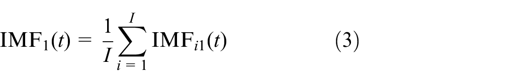
(3) The first residual $r_{1} (t)$ in the first stage can be obtained by equation (4) as follows.

r_{1} (t) = x (t) - {IMF}_{1} (t)

(4)

(4) Define $E_{i} (w_{i} (t))$ as the i-th IMF component after EEMD and $ε_{j}$ as the standard deviation of noise, The second IMF can be obtained by decomposing the sequence $r_{1} (t) + ε_{1} E_{1} (w_{i} (t))$

IM F_{2} (t) = \frac{1}{I} \sum_{i = 1}^{I} E_{1} (r_{1} (t) + ε_{1} E_{1} (w_{i} (t)))

(5)

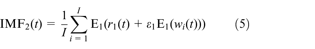
(5) The calculation formula for the k-th residual component (k = 2, 3, … K, K is the highest decomposition order) can be written as follows.

r_{k} (t) = r_{k - 1} (t) - IM F_{k} (t)

(6)

Therefore, the k + 1-th IMF component can be obtained by equation (7) as follows.

IM F_{k + 1} (t) = \frac{1}{I} \sum_{i = 1}^{I} E_{1} (r_{k} (t) + ε_{k} E_{k} (w_{i} (t)))

(7)

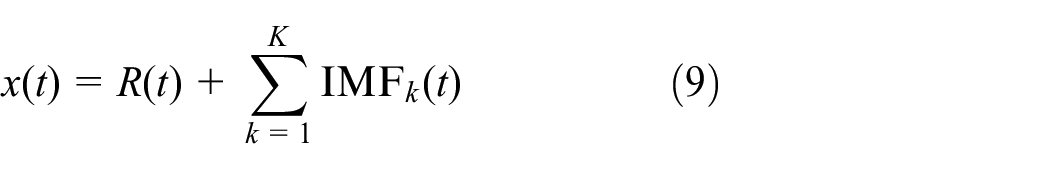
(6) Repeat steps 4–6 until the residual signal can’t be decomposed and the residual signal R(t) satisfies the relationship

R (t) = x (t) - \sum_{k = 1}^{K} IM F_{k} (t)

(8)

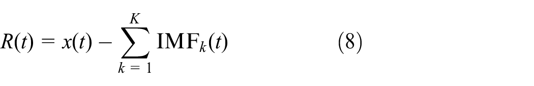
So the original signal can be expressed as

x (t) = R (t) + \sum_{k = 1}^{K} IM F_{k} (t)

(9)

The original vibration signal without noise and vibration signal with signal to noise ratio of 0 dB were decomposed by CEEMDAN, and the results are shown in Figure 3.

Figure 3.

CEEMDAN decomposition: (a) original vibration signal without noise and (b) vibration signal with signal to noise ratio of 0 dB.

Sample entropy

The size of signal sample entropy can indicate the degree of signal confusion. The more chaotic the signal, the stronger the noise in the signal, on the contrary, the smoother the signal, the weaker the noise in the signal. The calculation method of sample entropy is as follows.

(1) The k-th component obtained by decomposing the original signal is denoted by $IM F_{k} (t)$ , it can be expressed as

IM F_{k} (t) = {IM F_{k} (1), \cdot \cdot \cdot \cdot \cdot \cdot IM F_{k} (t), \cdot \cdot \cdot \cdot \cdot \cdot IM F_{k} (1024)}

(10)

Let the reconstruction dimension be m, then

IM F_{k, m} (t) = {IM F_{k} (t), IM F_{k} (t + 1) \cdot \cdot \cdot \cdot \cdot \cdot, IM F_{k} (t + m - 1)}

(11)

(2) Calculate the distance $l [IM F_{k, m} (t), IM F_{k, m} (j)]$ between $IM F_{k, m} (t)$ and $IM F_{k, m} (j)$ , it can be expressed as

\begin{matrix} l [IM F_{k, m} (t), IM F_{k, m} (j)] = \\ \max (| IM F_{k, m} (t + c) - IM F_{k, m} (j + c) |) \end{matrix}

(12)

where c = 0, 1, …, m, according to the rule of thumb, m = 2.

(3) Count the number B_i that $l [IM F_{k, m} (t), IM F_{k, m} (j)]$ is less than the threshold r, r = (0.1–0.25) × 1024, then the following formula can be obtained

B_{i}^{m} (r) = \frac{B_{i}}{1024 - m - 1}

(13)

$B^{m} (r)$ is defined as

B^{m} (r) = \frac{1}{1024 - m} \sum_{i = 1}^{1024 - m} B_{i}^{m} (r)

(14)

(4) Similarly, the number A_i whose distance between $IM F_{k, m + 1} (t)$ and $IM F_{k, m + 1} (j)$ is less than the threshold r can be calculated, and the definition of sample entropy can be obtained

SampEN (m, r) = - \ln [\frac{A^{m} (r)}{B^{m} (r)}]

(15)

According to the above method, the sample entropy of the original signal and signal with different noises can be calculated, and the calculation results are shown in Table 1.

Table 1.

Calculation results of sample entropy.

IMF	No noise	−4 dB	−2 dB	0 dB	2 dB	4 dB
IMF1	0.5936	1.3350	1.4751	1.3328	1.1911	1.2206
IMF2	0.1465	0.6619	0.6413	0.5587	0.5859	0.5299
IMF3	0.0296	0.3965	0.3023	0.3090	0.3577	0.2906
IMF4	0.0037	0.0841	0.1198	0.0757	0	0.0564
IMF5	0	0.0217	0.0167	0.0242	0.0159	0.0114
IMF6	0	0.0090	0.0023	0.0048	0.0044	0.0018
IMF7	0	0.0013	0	0.0038	0.0038	0
IMF8	/	0	0	0	0	0
IMF9	/	0	0	0	0	0
IMF10	/	0	0	/	/	/
IMF11	/	0	/	/	/	/
res	0	0	0	0	0	0

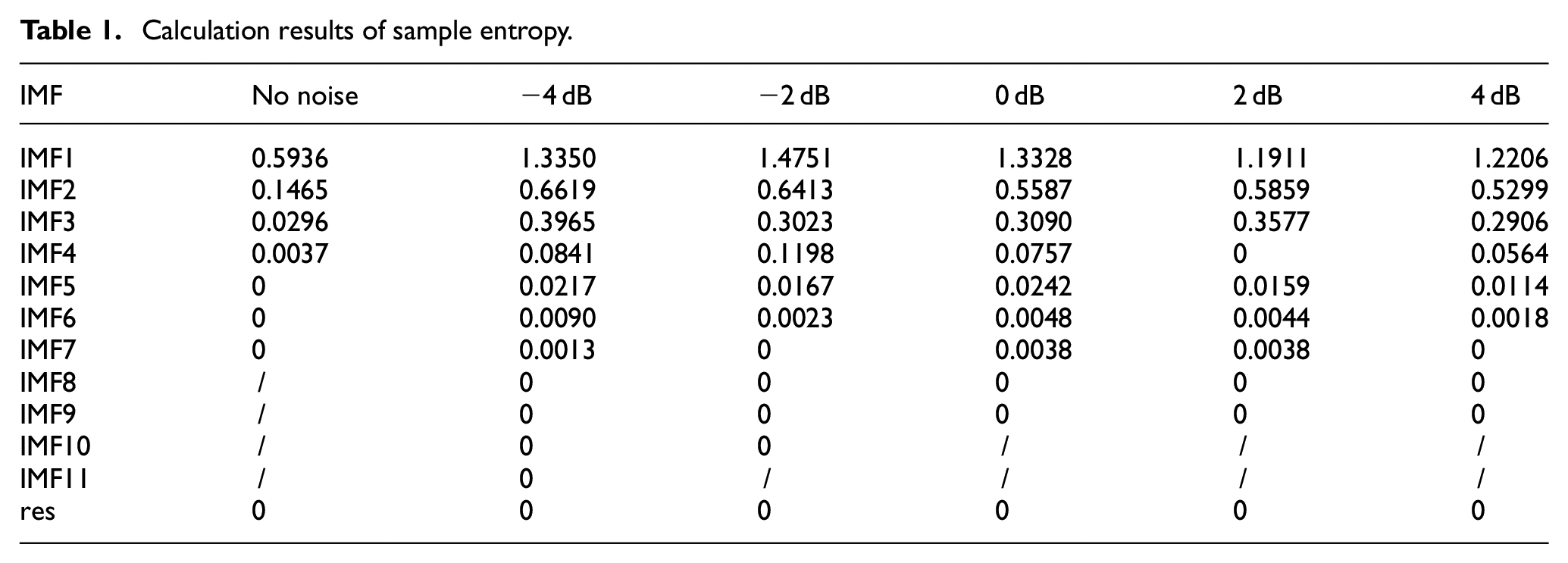
It can be seen from Table 1 that with the increase of CEEMDAN decomposition level, the sample entropy of IMF will return to zero, so reducing the noise in the low-level IMF can reduce the noise component in the reconstructed signal.

Adaptive wavelet de-noising

Noise signals often have high wavelet coefficients, while the traditional hard threshold and soft threshold wavelet de-noising methods need to set threshold η and compare it with the wavelet coefficient w_jk of the signal to filter the signal with η>|w_j,k|, so that the noise in the signal can be effectively filtered. Therefore, the setting of threshold η is very important. If η is too large, the noise will not be completely filtered, and if η is too small, the feature information in the signal will be partially filtered. In addition, the commonly used threshold $η = ε \sqrt{2 \log (N)}$ lacks adaptive ability and is not suitable for all damage cases. To solve this problem, this paper used an adaptive wavelet threshold, which is expressed as

\begin{matrix} η = \frac{(1 - 0.2 | r_{12} |) h_{j} \sqrt{2 \log (N)} median (| w_{j, k} |)}{0.6745 \ln (j + x)} \end{matrix}

(16)

where $ε = \frac{median (| w_{j, k} |)}{0.6745}$ , $median (| w_{j, k} |)$ is the median value of $| w_{j, k} |$ , the coefficient 0.6745 is the empirical constant, N is the length of signal, it equal to 1024, $r_{1, 2}$ is the correlation coefficient between the decomposed signal and the source signal.

The adaptive threshold function can be written as

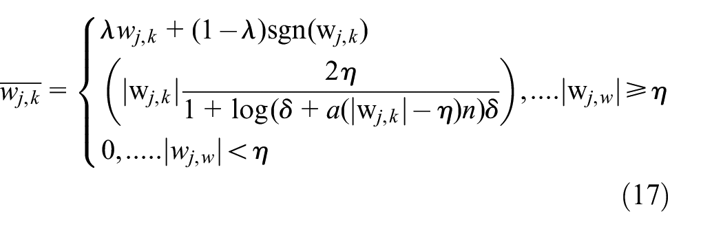
\begin{matrix} \bar{w_{j, k}} = {\begin{matrix} λ w_{j, k} + (1 - λ) sgn (w_{j, k}) \\ (| w_{j, k} | \frac{2 η}{1 + \log (δ + a (| w_{j, k} | - η) n) δ}), . . . . | w_{j, w} | \geq η \\ 0, . . . . . | w_{j, w} | < η \end{matrix} \end{matrix}

(17)

where $| w_{j, w} |$ is the adaptive wavelet coefficient, $λ = 1 - e^{- β \times {(| w_{j, k} | - η)}^{2}}$ , $η > 0$ , $δ > 0$ , $a > 0$ , $λ$ = 0–1.

The original signal and the signal with noise were filtered by adaptive wavelet, and the results are shown in Figure 4.

Figure 4.

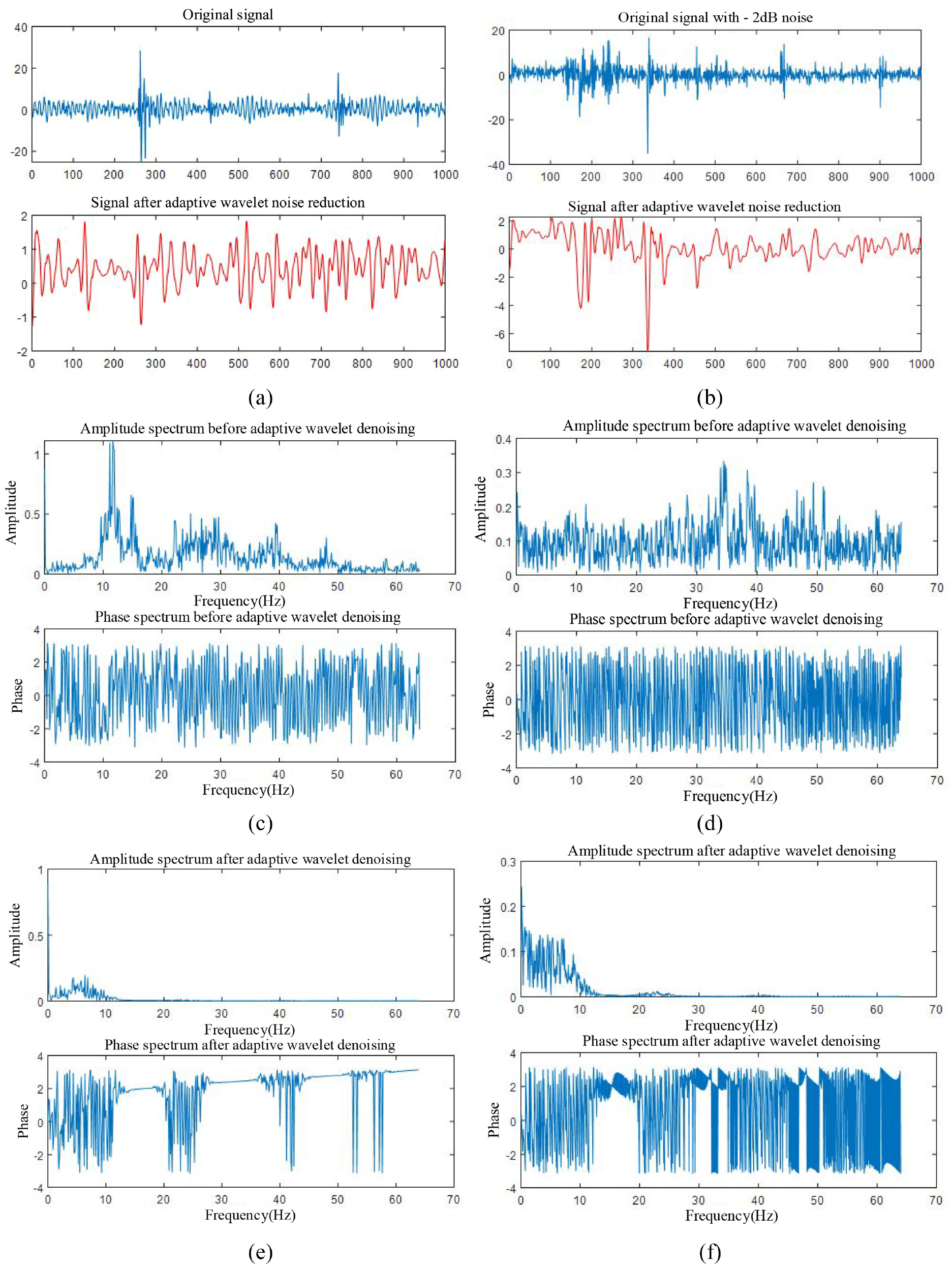
Wavelet de-noising and reconstruction: (a) wavelet decomposition and reconstruction without noise, (b) Wavelet decomposition and reconstruction with −2 dB noise, (c) Spectrum before wavelet decomposition without noise, (d) Spectrum before wavelet decomposition with −2 dB noise, (e) Spectrum of reconstructed signal without noise, and (f) Spectrum of reconstructed signal with −2 dB noise.

One dimensional convolution neural network

The convolution process of one-dimensional convolution neural network only needs to traverse the whole input in a certain step, and the receptive field of the first convolution layer is the length of the first convolution kernel. Convolution layer, pooling layer, BN layer, dropout layer, flattening layer and full connection layer are commonly used in one-dimensional convolution neural network. Convolution layer has the ability of feature extraction, and pooling layer plays a role in reducing the feature sharpening of tensor. Dropout layer can make the extracted features lose randomly in the convolution layer, so as to enhance the generalization ability of the network. Putting dropout in the full connection can make the neurons inactivate randomly according to the probability, so as to prevent the over fitting of the network. BN layer is usually placed behind the convolution layer to regularize the extracted features in the way of normal distribution, thus speeding up the training speed and fitting ability of the network. The flow chart of convolution neural network (CNN) algorithm is shown in Figure 5.

Figure 5.

Flow chart of CNN algorithm.

The convolution layer is defined as follows

x_{k}^{l} = b_{k}^{l} + \sum_{i = 1}^{N_{l - 1}} (W_{ik}^{l - 1} \times S_{i}^{l - 1})

(18)

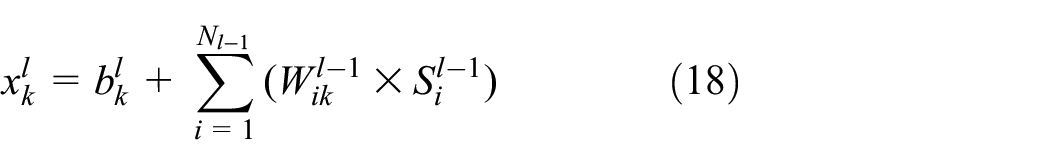
where $x_{k}^{l}$ is the input of the k-th neuron in layer l, $b_{k}^{l}$ is the deviation of the k-th neuron in layer l, $S_{i}^{l - 1}$ is the output of the i-th neuron in the layer l-1, $W_{ik}^{l - 1}$ is the weight of the i-th neuron in the layer l-1.

LSTM

Compared with CNN, LSTM pays more attention to the feature extraction of vibration signal with time series. When one-dimensional convolution neural network is used to extract the feature information of vibration signal, it is split in time, and can’t extract the correlation between tensor adjacent features, thus losing some features. Therefore, in this paper, based on the one-dimensional convolution neural network, the LSTM was added to its full connection layer to improve the feature extraction ability of the network. The flow chart of LSTM algorithm is shown in Figure 6.

Figure 6.

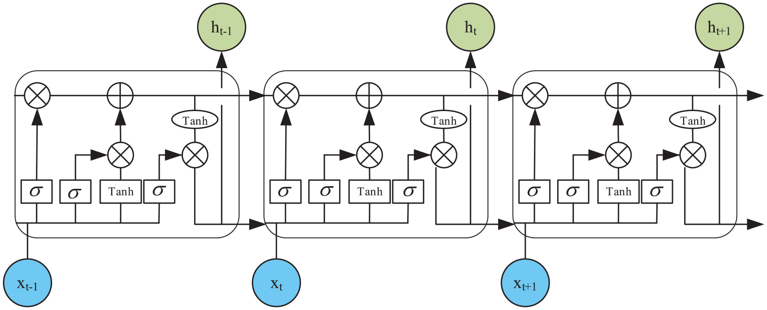
Flow chart of LSTM algorithm.

Compared with recurrent neural networks (RNN), LSTM is more flexible in state updating, and adopts forgetting gate to lose part of memory information randomly. In Figure 6, x_t is the input data at time t, and h_t is the output data. The update formula of LSTM is as follows

i_{t} = σ (W_{i} [h_{t - 1}, x_{t}] + b_{i})

(19)

o_{t} = σ (W_{o} [h_{t - 1}, x_{t}] + b_{o})

(20)

f_{t} = σ (W_{f} [h_{t - 1}, x_{t}] + b_{f})

(21)

C_{t} = f_{t} \otimes C_{t - 1} + i_{t} \otimes \tanh (W_{c} [h_{t - 1}, x_{t}] + b_{c})

(22)

h_{t} = o_{t} \otimes \tanh (C_{t})

(23)

where W_i, W_o, and W_f represent the weight coefficients of input gate, output gate and forgetting gate respectively, b_i, b_o, and b_f are bias vectors. Through this gate structure, LSTM neural network structure has the ability to maintain long-term storage information and effectively increase the memory length, which is suitable for extracting correlation features between combined signals.

WDCNN

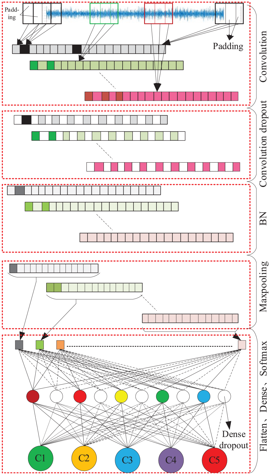
In this paper, based on WDCNN, the input of the first convolution layer was adjusted to 1024, which reduced the number of feature extraction in the first convolution layer by half. Therefore, the size of the kernel added after the first convolution layer is 64, the step size is 4, the middle transition layer with 32 channels made the perception field of the whole network return to the level of WDCNN. In addition, because the ability of suppression fitting of dropout in the convolution layer is not obvious, dropout was added to the fully connection layer to suppress the occurrence of over fitting. The convolution process of the improved WDCNN is shown in Figure 7.

Figure 7.

Convolution process of the improved WDCNN.

In this paper, two LSTMs were used to replace the two full connection layers of the neural network, and the dropout layer was added between two LSTMs, so that the time data transmission of two LSTMs was lost immediately according to a certain probability, so as to increase the generalization ability of the network. At the same time, the Adam adaptive optimization algorithm³⁰ was used to optimize the weight parameters of the whole network.

Training results

Training conditions

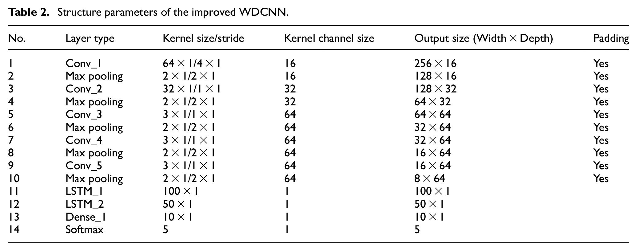
In this paper, Tensorflow 2.4.8, keras 3.4.2 and Python 3.8.0 were used as the training data preprocessing and convolution neural network implementation environment. In order to train the neural network model proposed in this paper, a laptop was used to run the program. The configuration of the laptop is CPU: Intel Corei7-4710MQ, GPU: NVIDIA GT940M 2G and memory: 12G. During training, the parameters shown in Table 2 were used as the structural parameters of the convolutional neural network, the batch size is 128, the dropout is 0.5, and the training epoch is 1000. In addition, the optimizer used in this paper is Adam. Because Adam has adaptive ability, and using Adam’s default initial learning rate for adaptive learning has the advantages of fast training speed, obvious change of training curve, strong ability to resist over fitting, this paper used the default initial learning rate of the operating environment.

Table 2.

Structure parameters of the improved WDCNN.

No.	Layer type	Kernel size/stride	Kernel channel size	Output size (Width × Depth)	Padding
1	Conv_1	64 × 1/4 × 1	16	256 × 16	Yes
2	Max pooling	2 × 1/2 × 1	16	128 × 16	Yes
3	Conv_2	32 × 1/1 × 1	32	128 × 32	Yes
4	Max pooling	2 × 1/2 × 1	32	64 × 32	Yes
5	Conv_3	3 × 1/1 × 1	64	64 × 64	Yes
6	Max pooling	2 × 1/2 × 1	64	32 × 64	Yes
7	Conv_4	3 × 1/1 × 1	64	32 × 64	Yes
8	Max pooling	2 × 1/2 × 1	64	16 × 64	Yes
9	Conv_5	3 × 1/1 × 1	64	16 × 64	Yes
10	Max pooling	2 × 1/2 × 1	64	8 × 64	Yes
11	LSTM_1	100 × 1	1	100 × 1
12	LSTM_2	50 × 1	1	50 × 1
13	Dense_1	10 × 1	1	10 × 1
14	Softmax	5	1	5

Accuracy

Training curve is an important index to show the stability and accuracy of neural network training. The recognition rate of the network can be obtained through the accuracy curve, and the stability of network training can be obtained by analyzing the change curve of objective function value (Loss). The training curves of 750–1000 epochs in the training process of five types of fault diagnosis under different working conditions are shown in Figure 8.

Figure 8.

Training curves: (a) accuracy curves and (b) loss curves.

By analyzing the training curves in Figure 8, it can be seen that the accuracy of the training set is stable between 0.998 and 1 under no load condition. When the load is 0.2 A, the accuracy of the training set changes greatly. When the load is 0.1 A, the accuracy of the training set fluctuates between 0.994 and 1. Therefore, it can be concluded that the vibration data under no load condition is more conducive to neural network fitting. But the accuracy of the test set under all working conditions are between 0.998 and 1, which shows that the proposed method has a very high recognition rate. At the same time, by analyzing the change curve of Loss, it can be seen that the network model is more stable under no load condition, and the Loss of the test set is reduced to 0.005–0. Therefore, it can be concluded that the method proposed in this paper has small error in gearbox fault diagnosis.

Visualization

Using TSNE to visualize the training results can obtain the distance between each fault category. The larger the distance is, the higher the reliability of the classification results is. On the contrary, there is a large error. In this section, WDCNN and the method proposed in this study were used to train five kinds of fault data under no load condition. When the training epochs are 50, the output clustering results of the last layer of the full connection layer obtained by using the two models are shown in Figure 9.

Figure 9.

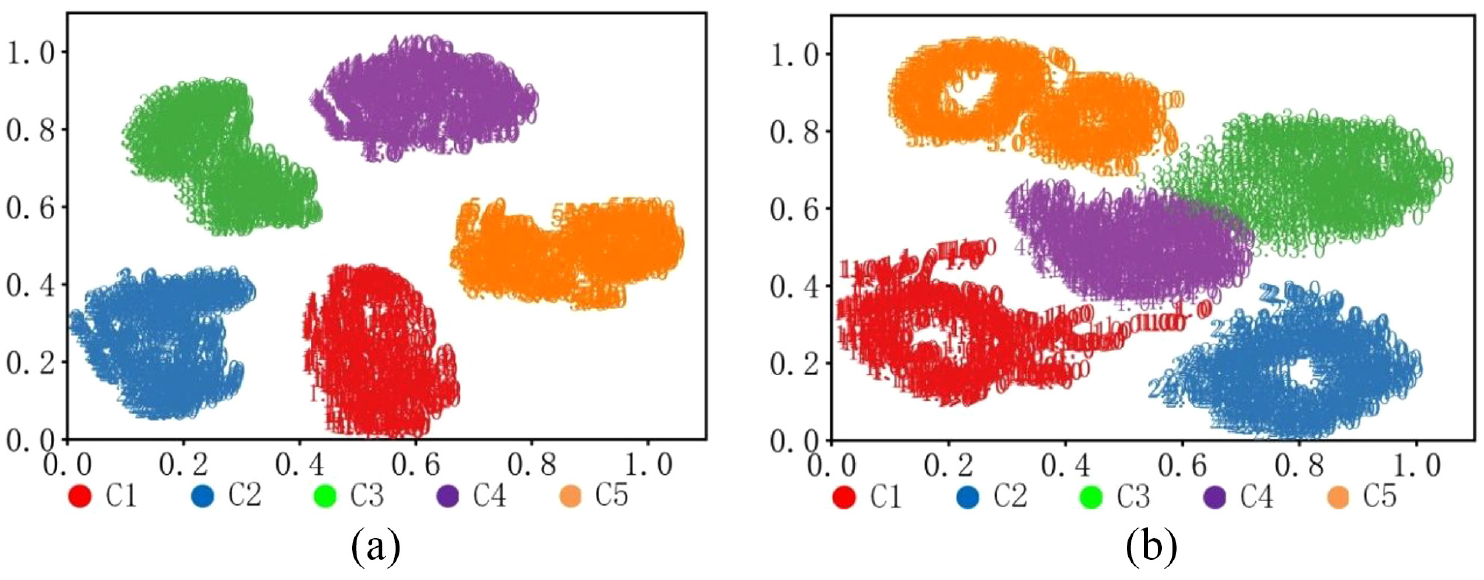
TSNE visualization: (a) classification results of the method proposed in this paper and (b) classification results of WDCNN.

Through the results of visualization in Figure 9, it can be seen that the distance between the five faults obtained by using the method proposed in this paper is much greater than that obtained by using WDCNN, this shows that the method proposed in this paper can more accurately identify and classify gearbox fault signals, and the effect is better than WDCNN.

Fault diagnosis results

The noise interference of the gearbox in actual use can be simulated by adding noise with different signal-to-noise ratio to the no load original vibration signal. In this paper, different methods were used to diagnose gearbox faults under different signal-to-noise ratio. The diagnosis results are shown in Tables 3 and 4.

Table 3.

Accuracy under different signal-to-noise ratio by using different methods.

Method	No noise	−4 dB	−2 dB	0 dB	2 dB	4 dB
WDCNN	0.8561	0.5764	0.6359	0.7021	0.8091	0.8477
WDCNN + LSTM	0.9921	0.8769	0.8963	0.8932	0.9302	0.9545
CEEMDAN + WDCNN + LSTM	1.0000	0.9854	0.9887	0.9603	0.9937	0.9975
CEEMDAN + 5-level wavelet + WDCNN + LSTM	1.0000	0.9997	1.0000	1.0000	1.0000	1.0000
CEEMDAN + 4-level wavelet + WDCNN + LSTM	1.0000	0.9925	0.9947	0.9976	0.9988	0.9994
CEEMDAN + 3-level wavelet + WDCNN + LSTM	1.0000	0.9911	0.9925	0.9943	0.9986	0.9993
CEEMDAN + 2-level wavelet + WDCNN + LSTM	1.0000	0.9899	0.9912	0.9925	0.9974	0.9988
CEEMDAN + 1-level wavelet + WDCNN + LSTM	1.0000	0.9866	0.9893	0.9901	0.9941	0.9980

Table 4.

Loss under different signal-to-noise ratio by using different methods.

Method	No noise	−4 dB	−2 dB	0 dB	2 dB	4 dB
WDCNN	0.1446	2.2734	2.5321	0.7787	0.5023	0.4136
WDCNN + LSTM	0.1014	0.1689	0.1023	0.0955	0.0788	0.0776
CEEMDAN + WDCNN + LSTM	0.0701	0.0634	0.0623	0.0503	0.0473	0.0401
CEEMDAN + 5-level Wavelet + WDCNN + LSTM	1.1 × 10⁻⁶	1.5 ×1 0⁻⁴	7.3 × 10⁻⁵	4.7 × 10⁻⁵	1.8 × 10⁻⁵	9.8 × 10⁻⁶
CEEMDAN + 4-level Wavelet + WDCNN + LSTM	0.0056	0.0130	0.0106	0.0066	0.0046	0.0021
CEEMDAN + 3-level Wavelet + WDCNN + LSTM	0.0163	0.0180	0.0161	0.0154	0.0101	0.0096
CEEMDAN + 2-level Wavelet + WDCNN + LSTM	0.0253	0.0401	0.0367	0.0254	0.0289	0.0203
CEEMDAN + 1-level Wavelet + WDCNN + LSTM	0.0444	0.0619	0.0546	0.0503	0.0461	0.0312

It can be seen from Tables 3 and 4 that the method proposed in this paper has been used for fault diagnosis of the gearbox under different signal-to-noise ratio. In order to verify the superiority of the method proposed in this paper in terms of noise resistance, at the same time and under the same conditions, WDCNN, WDCNN + LSTM, CEEMDAN + WDCNN+LSTM were respectively used for fault diagnosis of the gearbox, and the diagnosis results were compared with the method proposed in this paper. The research results show that LSTM can extract the correlation features between the feature information obtained by WDCNN, which increases the overall accuracy of the model. The method of using CEEMDAN components to lose part of the features also has a certain anti-noise ability. Compared with the traditional wavelet decomposition and reconstruction, the adaptive wavelet decomposition and reconstruction method proposed in this paper has stronger anti-noise ability and higher recognition rate. Under the environment of no noise and low noise, the fault diagnosis accuracy of the gearbox by using the method proposed in this paper is 100%; even if the signal to noise ratio is −4 dB, the fault diagnosis accuracy of the gearbox can still reach 99.97%. Therefore, the fault diagnosis method proposed in this paper has strong accuracy and anti-noise ability, and can achieve accurate diagnosis of gearbox faults in noise environment.

Conclusions

Aiming at the noise problem in gearbox fault diagnosis, this paper proposed a new gearbox fault diagnosis method, which uses CEEMDAN to decompose the original vibration signal, uses adaptive wavelet to de-noise the IMF with high sample entropy and reconstructs the de-noised components, uses WDCNN to extract the digital features of the reconstructed signal, and uses LSTM to extract the correlation between features. The fault diagnosis experiments of the gearbox were carried out under different load conditions and noise environments by using the fault diagnosis method proposed in this paper and compared with other methods. The experimental results show that the accuracy of the fault diagnosis method proposed in this paper is 100% in the case of no noise and low noise, and 99.97% in the case of the signal to noise ratio is −4 dB. Therefore, the fault diagnosis method proposed in this paper has strong anti-noise ability and high recognition rate, which is superior to other methods, and can provide a basis for fault diagnosis research of gearbox under noise environment.

The conclusions of this paper are obtained when Gaussian white noise is added to the original data, but in the actual environment, the noise is complex, in addition to Gaussian white noise, there are other different types of noise. Meanwhile it is difficult to rely on only one kind of environmental noise for fault diagnosis. Therefore, in the next research, fault diagnosis of gearbox under different types of noise environment will be studied.

Footnotes

Handling Editor: Chenhui Liang

Declaration of conflicting interests

The author(s) declared no potential conflicts of interest with respect to the research, authorship, and/or publication of this article.

Funding

The author(s) disclosed receipt of the following financial support for the research, authorship, and/or publication of this article: This work was supported by the Nature Science Foundation of Hebei Province grant no. E2020402060, and Key Laboratory of Intelligent Industrial Equipment Technology of Hebei Province (Hebei University of Engineering) under Grant 202204 and 202206.

ORCID iD

Chaozhi Cai

References

Bao

, et al. Parametric short time Fourier transform and gearbox fault diagnosis. Vibr Test Diag 2020; 40: 272–277.

Fault diagnosis of wind turbine gearbox based on empirical wavelet transform and correlation dimension. J Power Eng 2021; 41: 113–120.

Liu

Zeng

Cui

, et al. Gear fault diagnosis based on empirical mode decomposition and differential envelope spectrum. Comp Measur Contr 2021; 29: 54–58.

Zhong

Xia

Mei

An effective centre frequency selection scheme based on variational mode extraction and its application to gear fault diagnosis. Insight 2022; 64: 155–163.

Zhong

Huang

Mei

, et al. A gearbox fault diagnosis method based on MKurt spectrum and CYCBD. Insight 2021; 63: 472–478.

Zhang

Liu

Meng

, et al. Deep learning-based automatic recognition network of agricultural machinery images. Comput Electron Agric 2019; 166: 104978.

Zhou

, et al. A quantum deep convolutional neural network for image recognition. Quant Sci Technol 2020; 5: 044003.

Wang

Gao

RX.

Machine vision intelligence for product defect inspection based on deep learning and Hough transform. J Manuf Syst 2019; 51: 52–60.

Nasirahmadi

Sturm

Edwards

, et al. Deep learning and machine vision approaches for posture detection of individual pigs. Sensors 2019; 19: 3738.

10.

Pathak

Pandey

Rautaray

Application of deep learning for object detection. Procedia Comput Sci 2018; 132: 1706–1717.

11.

Haris

Glowacz

Road object detection: A comparative study of deep learning-based algorithms. Electronics. Electronics 2021; 10: 1932.

12.

Ionescu

Deep learning algorithms and big health care data in clinical natural language processing. Linguist Philos Investig 2020; 19: 86–92.

13.

Vicari

Gaspari

Analysis of news sentiments using natural language processing and deep learning. AI Soc 2021; 36: 931–937.

14.

Zhao

Liu

Bearing fault diagnosis method based on VGG16 transfer learning. Spacecr Environ Eng 2020; 37: 446–451.

15.

Zhang

Peng

, et al. A deep convolutional neural network with new training methods for bearing fault diagnosis under noisy environment and different working load. Mech Syst Signal Process 2018; 100: 439–453.

16.

Cai

Zhao

Intelligent diagnosis method based on GaN sample generation technology. Vibr Shock 2020; 39: 153–160.

17.

Deep learning based approach for bearing fault diagnosis. IEEE Trans Ind Appl 2017; 53: 3057–3065.

18.

Chen

Mauricio

, et al. A deep learning method for bearing fault diagnosis based on cyclic spectral coherence and convolutional neural networks. Mech Syst Signal Process 2020; 140: 106683.

19.

Hoang

Kang

HJ.

A motor current signal-based bearing fault diagnosis using deep learning and information fusion. IEEE Trans Instrum Meas 2020; 69: 3325–3333.

20.

Nguyen

Hoang

Tran

, et al. A bearing fault diagnosis method using multi-branch deep neural network. Machines 2021; 9: 345.

21.

Saufi

Ahmad

ZAB

Leong

, et al. Gearbox fault diagnosis using a deep learning model with limited data sample. IEEE Trans Ind Inform 2020; 16: 6263–6271.

22.

Singh

Azamfar

Ainapure

, et al. Deep learning-based cross-domain adaptation for gearbox fault diagnosis under variable speed conditions. Meas Sci Technol 2020; 31: 055601.

23.

Mallikarjuna

Sreenatha

Manjunath

, et al. Aircraft gearbox fault diagnosis system: an approach based on deep learning techniques. J Intell Syst 2021; 30: 258–272.

24.

Yang

Zhang

Wind turbine gearbox failure detection based on SCADA data: A deep learning-based approach. IEEE Trans Instrum Meas 2021; 70: 1–11.

25.

Zhang

Sheng

Huang

, et al. Fault diagnosis model of pressure reducing valve unbalance sample based on W-DenseNet. Control and decision 2022; 37: 1513–1520.

26.

Zhu

Liu

Fault diagnosis of rolling bearing based on CEEMDDAN Hilbert CNN. J Qingdao Univ Sci Technol 2021; 42: 97–103.

27.

Zhang

Research on bearing fault diagnosis algorithm based on convolution neural network. Harbin: Harbin Institute of technology, 2017.

28.

Zhang

Lin

Luo

Application of improved LSTM neural network in motor fault diagnosis. Comp Measur Contr 2021; 29: 45–50.

29.

BWang

Zhao

, et al. Fault diagnosis method of reciprocating compressor bearing based on CEEMDDAN and RCMDE. Mach Tool Hydraul 2021; 49: 168–172.

30.

Zheng

Zhang

Pan

Fault diagnosis of rolling bearing based on improved whale algorithm optimized LSTM. Vibr Shock 2021; 40: 274–280.

Fault diagnosis of gearbox based on adaptive wavelet de-noising and convolution neural network

Abstract

Keywords

Introduction

Experimental data

Fault diagnosis process

Data preprocessing

CEEMDAN

Sample entropy

Adaptive wavelet de-noising

One dimensional convolution neural network

LSTM

WDCNN

Training results

Training conditions

Accuracy

Visualization

Fault diagnosis results

Conclusions

Footnotes

Declaration of conflicting interests

Funding

ORCID iD

References