
Abstract
Uncertainty exists in many industry fields and needs to be dealt properly to avoid unexpected failure. This article proposes a new approach to deal with the uncertain problems encountered by the mathematical modeling of an active hydraulically interconnected suspension system. As the need for both riding comfort and the controllability is soaring nowadays, the traditional passive and semi-active suspension system could barely keep up with the pace, and the proposed active hydraulic system could be one of the solutions. In order to deal with the uncertain factors in the hydraulic system, an interval analysis method for the dynamic responses of nonlinear systems with uncertain-but-bounded parameters using Chebyshev polynomial series is introduced. The comparisons conducted in this article demonstrate the accuracy and computational efficiency of the proposed uncertain problem solver and reveal the influences of uncertain parameters in fluid and mechanical components on the dynamic responses of active hydraulically interconnected suspension.
Keywords
Introduction
Vehicle has become inalienable in modern society as it extends people’s home range with incredible convenience. As a result, the reliability and the performance of riding attract enormous attention from manufactures, and to some extent decide the popularity of one vehicle. The key in improving the controllability of a vehicle and the riding quality largely depends on suspension which connects a vehicle body to its wheels and isolates the vibration from rough ground, 1 and it also accounts for most fatal crashes, which is around 33%, 2 related to uncontrollable motions (roll, pitch, bounce, and articulation). 3 The situation of rollover, which is the most dangerous, even gets worse with the increasing popularity of sport utility vehicles as they have higher centers of gravity (CGs). 4 To solve the aforementioned problems, an adequate adjusted suspension system is imperative. 5
Modern suspension system could be classified into three categories which are passive suspension, semi-active suspension, and active suspension. The prevailing type nowadays goes to passive suspension 6 giving credit to its cost-effectiveness and reliabilities. However, the drawbacks of this kind of system are also evident, one of which is the compromise between riding comfort and handling stability, 7 because the increase in suspension roll stiffness and damping will inevitably result in abrupt bumping over rough geography. The other drawback could be illustrated by anti-roll bar, which would undesirably stiffen the suspension warp mode and weaken the road holding ability. As a complement to the passive suspension, semi-active suspension 8 was brought out. It utilizes the adjustability of the area of orifice in the damper to control the damping force in order to achieve the control over the suspension. But it fails to introduce external energy into the suspension system which differentiates it from the active suspension.9,10 The most remarkable feature of an active suspension system is that the suspension force is provided, 11 at least a portion, by active power sources. It enables the active activities based on the signals acquired by various sensors attached to the key points of the vehicle to measure the motion of the body and suspension, and a control unit will process these data and then adjust the parameters according to the driving condition. 12 There are extensive surveys about the conventional active suspension, and many of them achieved great improvements compared with passive and semi-active ones. However, the conventional active suspensions have their own limitations which constrain the application within a narrow scope such as sport vehicles and luxury vehicles. Typical conventional active suspension has independent structures including four independent controlled actuators, attributing to soaring cost, reduced reliability, increased power consumption, and inherent complexity. The desired control force would be directly applied to the vehicle chassis to achieve superior performance only if the system could satisfy the significant power requirement. Instead of adopting independent layout of four actuators, the idea of introducing compact interconnected fluid circuits into suspension design helps solve the aforesaid problems properly. A good example could be the dynamic ride control (DRC) sport suspension system. The diagonally interconnected mechanical structure adopts a pump as the external pressure source to provide force into the diagonally linked shock absorbers to achieve a stable motion during cornering, avoiding rollover.
To take the progress one step further, a more sophisticated and robust active hydraulically interconnected suspension (HIS) model is proposed; 13 it cooperates four hydraulically interconnected actuators, which are interconnected by two circuits in roll plane, into each wheel station and a control unit comprised a motor, a bump, a servo valve, a tank, an accumulator, and so on, achieving the goal of structure simplicity and reduced overall cost. It could actively tilt the vehicle against the uncontrollable rollover by providing desired restoring forces, 14 while not consuming much energy, because the variable here is the vertical force, not the suspension deflection, which means not much work should be done. 15
Due to the presence of fluid flow and the companying uncertain parameters such as pipe friction and working fluid damping coefficient, 16 large uncertainty is introduced into the mathematical modeling. The nonlinear nature of the hydraulic system weakens the accuracy of the mathematical model of the actuator that is crucial in analyzing. In this article, to solve the uncertain problems encountered during mathematical modeling, an interval analysis method for dynamic response of nonlinear systems with uncertain-but-bounded parameters is proposed using Chebyshev expansion series.
Uncertainties are inherent in nearly all the real-world problems 17 such as loads, material properties, boundary conditions, fraction, geometry, and the problem of uncertainty especially looms large because of the increase in complexity and precision of modern systems. 18 Unfortunately, even small uncertainties of parameters may attribute to large variation in system dynamic change due to the characteristics of enlargement of propagation. 19 Many methods have been brought out mainly fitting into two categories: probabilistic methods 20 and non-probabilistic methods. 21 The probabilistic methods have acquired decent achievements in practical engineering, but it is limited by the needs to express uncertain parameters as stochastic variables with precise probability distribution, which means to know the complete information.
Interval method, 22 as a non-probabilistic method, taking advantages of the ease of acquiring the boundary of the uncertainties, shows great potential in dealing with this problem and has been verified by a range of engineering design problems. 23 The minimal and maximal responses of the uncertain objective and constraints are the corresponding bounds of an interval function; in other words, the interval method calculates the upper bound and lower bound of the true solution. The bounds can be obtained by using the interval arithmetic or optimization method. However, encountered by most interval arithmetic, overestimation, 24 which is caused by the so-called “wrapping effect,” 25 compromises the accuracy, especially in the process of numerical iterations where it would be accumulated. Although the Taylor interval method26–28 and Chebyshev interval method are proposed to control overestimation, it is still hard to eliminate the overestimation completely. The optimization method may obtain higher accurate bounds, but its efficiency would be quite low, especially for complicated engineering problems.
In this article, Chebyshev series expansions are introduced to build a surrogate model of the active HIS model. Chebyshev surrogate model achieves a higher numerical accuracy when dealing with uncertain problems. The scanning method, which is more accurate than interval arithmetic, is used to compute the bounds based on the Chebyshev surrogate mode, and it is much more efficient than the scanning method based on original complicated model.
Modeling of active hydraulic interconnected suspension
A representative model is the fundamental of precise and thorough investigation. Due to the characteristic of symmetry of a conventional vehicle chassis, a half-car model is adopted here to simplify the analysis process without the risk of losing generality.
Simplified half-car model
Figure 1 shows the proposed half-car model.

Half-car model.
As a number of dynamic systems are governed by ordinary differential equations, by using Newton’s second law, the motion equations of this model could be derived as follows
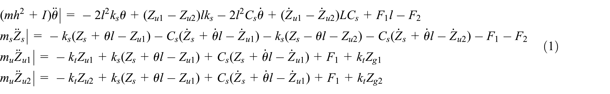
where
Modeling of hydraulic system
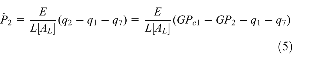
There are three main components which comprise the active suspension which are as follows: four double-direction hydraulic actuators, two interconnected hydraulic circuits, and a compact pressure control unit. Figure 2 is the schematic drawing of the active HIS. Hydraulic actuators possess the advantages of low cost and energy efficiency, which are crucial in commercial application. By adopting advanced control strategies, a mechanical hydraulic system could achieve even better performances. However, hydraulic actuators have the inherent drawback which is nonlinear and complicated dynamics. This, to a considerable extent, influences the dynamic response analysis of the whole system.

Schematic diagram of active HIS.
The four actuators, which are controlled by the pressure control unit, are mounted according to the specific structure of a vehicle between the wheels and the chassis. The active suspension could promptly act to tilt the vehicle to prevent it from rollover. Take the condition in Figure 2 as an example, the vehicle body shows the trend to roll to the left side, the pressure of circuit A would rise, under the command of control unit, to stiffen left side suspension, while the pressure of circuit B would be reduced to keep the body in balance. The anti-moment could be expressed as follows

where
The compact control unit energizes the actuators according to the angle sensors; in other words, it reacts to the demand of the actual road conditions. This feature could also be called demand dependence, which could help the system avoid oversensitive reactions. There are two reasons for avoiding oversensitive reactions; the first one is that “nulling” tilt would consume considerable energy while help little in handling the motion of the vehicle. The other reason is the feeling of acceleration also plays an important role in driving experience, 29 which would be compromised by oversensitivity. As a result, the active HIS would help vehicles maintain controllable motion while have comparable efficiency with much lower energy consumption.
Involving the hydraulic system, which possesses high-level uncertainties, makes the numerical analysis more sophisticated. In order to make the expression more concise, the uncertain parameter vector, which is k-dimensional, could be expressed as follows

where

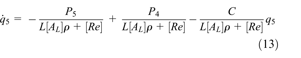
Figure 3 shows the flow and input sign convention in the HIS.

The flow and input sign convention in the HIS.
It can be seen that

where
Take cylinder chamber

where
In the hydraulic system, the other influential uncertainties come from the pipe friction and the working fluid damping coefficient, and a little change happening in these parameters would lead to large fluctuations in the system dynamic responses. What makes the situation worse is that it is hard to acquire full information about these parameters. Express the uncertain parameters of pipe friction and working fluid damping coefficient with [Re] and [C], respectively, then the flow into the piston chamber could be given as follows


The flows into other chambers could be calculated similarly


Integrated modeling
After the mathematical modeling of the half-car model and the active HIS system, it is feasible to couple these two systems together. The roll angle acquired by the sensors could be used as the input of the active HIS, and the hydraulic forces, which are shown below, provided by the active HIS are the restoring forces for the car model


In order to obtain the assembled system, on the fundamental of the coupling interactions between the half-car model and the active HIS system, the equations concerning these two models should be combined together and be expressed in matrix form. The state vectors could be like


The state of the HIS system could be expressed like


where


where
The complete model of the proposed system in the form of

The proposed active HIS-assisted half-car model is developed with Simulink.
Chebyshev surrogate model
As demonstrated in the previous sections, the high uncertainties introduced by the hydraulic system should be adequately dealt with to develop a robust and reliable analysis model. In engineering, the uncertainties induced by bounded parameters could be handled by convex model or interval model. Traditionally, low-level Taylor series–based interval method can only solve the problems whose uncertain levels are small; otherwise, the overestimation phenomenon would be frustrating. In this section, Chebyshev series expansion 30 is introduced to build a surrogate model of the hydraulic interconnected suspension system, and then it is combined with scanning method to compute the bounds.
Considering the responses of the model as a continuous function without knowing its analytical expression, let us assume that there exists a polynomial

where
Let

where

where
The Chebyshev polynomial could be expressed by

For the multi-dimensional problem, the concept on tensor product should be adopted. By generating the tensor products of the one-dimensional equations, the Chebyshev polynomial for a k-dimensional problem is expressed as
where
Because of the orthogonality of this series, the following equation holds

where
The truncated Chebyshev series expansion of

where
The truncated error 31 is

As to the calculation of the constant coefficients

where

where

So the coefficients of Chebyshev polynomials are as follows

Equation (37) is a linear combination of the values of the function which makes the calculation Chebyshev coefficient easy to obtain.
For a k-dimension problem

In order to minimize the integral error,
The algorithm can be summarized as:

Interval uncertain analysis of active HIS
In this section, the proposed Chebyshev interval method is used in the active HIS system to deal with the uncertain parameters aforesaid to develop a robust and reliable model.
Parameter tuning
In order to guarantee the proposed model could adequately represent the real situation, parameter tuning should be conducted at first. Table 1 shows the parameters adopted in this article.
Integrated system parameters.
CG: center of gravity.
Most of the parameters are obtained through previous work,
15
such as the suspension spring stiffness, the suspension damper coefficient, and the valve controller gain. In this article, the main concentration is focused on the uncertain parameters whose little change would introduce large fluctuation in the system dynamic responses. These parameters are separated into two sets according to their nature, which is hydraulic or not, for the sake of adequate demonstration. The first set includes upper piston cross-sectional area (m2), which can be expressed as
Uncertain analysis of fluid parameters
The anti-roll mode would be activated when the vehicle experiences rolling under the operation of turning. In this simulation, the vehicle is supposed to have a right turn; as a result, it would have a tendency to roll to the left side. In order to counteract this tendency, the HIS system would rise the pressure of the upper chamber on the left side and reduce the pressure on the right side to provide the entailed supportive force on the left. To simulate this action, a 25-bar signal and a 50-bar signal are sent to the lower chamber circle and upper chamber circle on the left side through the servo valve, respectively. The order of the Chebyshev inclusion function is set to
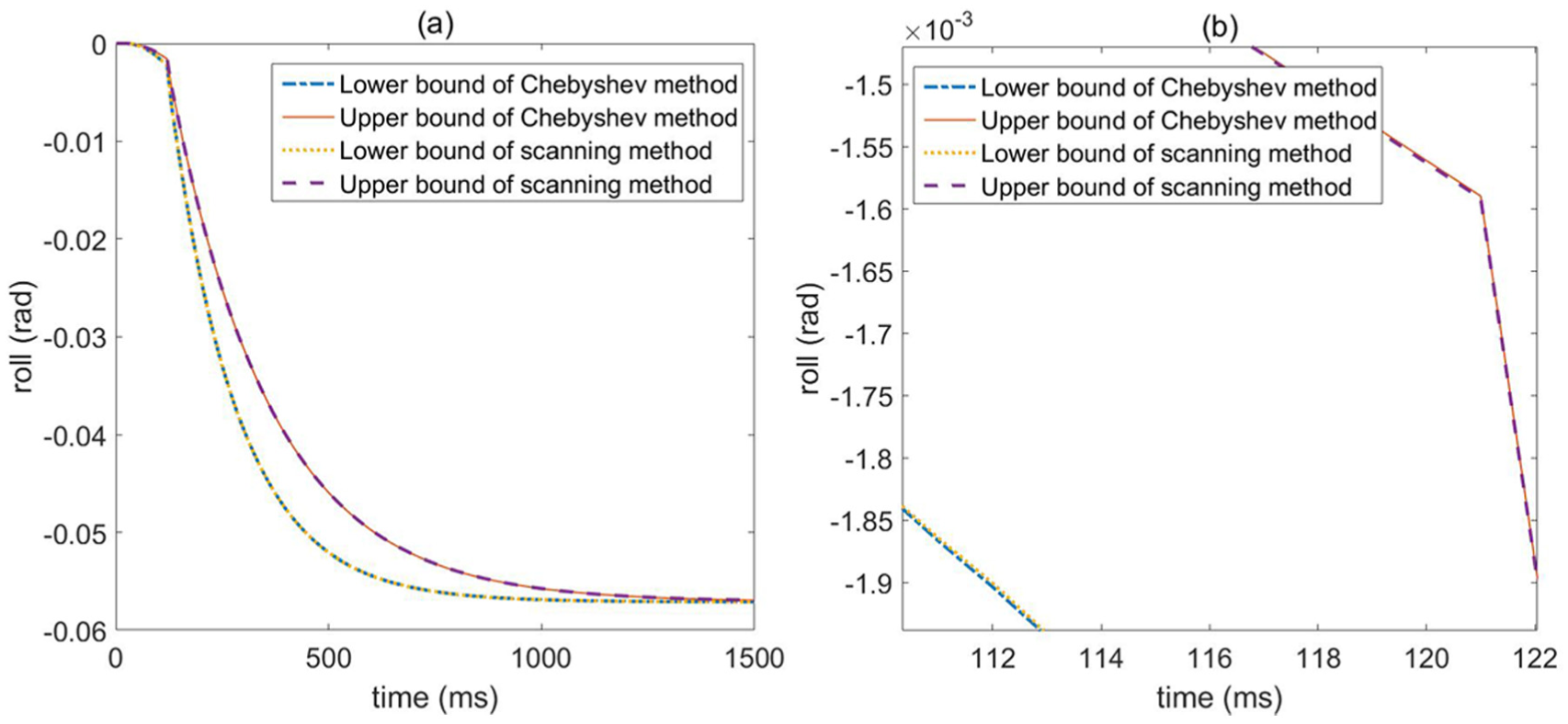
It can be seen in Figure 4(a) that the deflection experiences an oscillation at the beginning of the process and then a steep ascent until the predetermined value. It is evident that there exists a considerable area between the upper bounds and the lower bounds, which is caused by the uncertain parameters of [C] and [Re] even under the condition that the uncertain range was set to a relative low level. If the uncertainty rises, the differences between these two bounds would be even greater. As to the upper bound, it takes about 800 ms to reach the stable state which is expressed by the horizontal trend; the lower bound takes around 1200 ms to reach a relative stable state. It should be point out that there are actually two upper bounds and two lower bounds in Figure 4(a) which can only be seen in the amplified plot Figure 4(b) because the differences between them are very small. In Figure 4(b), the upper bound and the lower bound which enclose the other two bounds are generated by the proposed Chebyshev inclusion method, and the enclosed two bounds are the results of the comparison set named scanning method, which represent the relatively accurate real situation. The little difference between these two methods demonstrates the good approximation ability that the Chebyshev surrogate model possesses. Another merit that lies in the proposed method is the computational efficiency. The iterative numbers of the Chebyshev method and the scanning method are

Deflection responses of both sides with uncertain parameters of [C] and [Re]: (a) deflection on left side, (b) amplified plot on left side, (c) deflection on right side, and (d) amplified plot on right side.
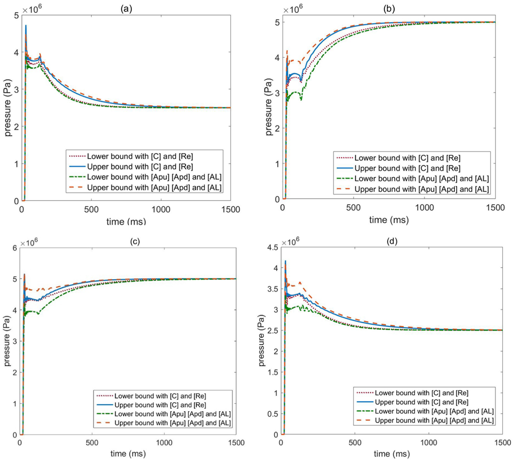
Figure 5 shows the dynamic pressure responses in the four chambers of the two actuators. As to the left actuator, the stable pressure of the upper chamber is 25 bar and the stable pressure of the lower chamber is 50 bar. The pressure difference between these two chambers makes the actuator to extend or, in other words, to stiffen the suspension. To the right side, it is exactly the opposite situation. It can also be seen that, to the upper chambers, the transient pressure would reach around 50 bar and then decrease about 10 bar. The pressure of the lower chambers, at first, would only reach around 40 bar. The oscillation during the establishment of the stable pressure is obvious, which is the characteristics of hydraulic. The influences introduced by the uncertain parameters are much the same as the deflection situation demonstrated; the upper bounds and the lower bounds draw the possible region where the real pressure response trajectory might be. The effectiveness of the proposed Chebyshev internal method is illustrated in Figure 6.

Pressure responses of the four chambers of two actuators with uncertain parameters of [C] and [Re]: (a) left upper chamber, (b) left lower chamber, (c) right upper chamber, and (d) right lower chamber.

Amplified pressure responses of the four chambers of two actuators with uncertain parameters of [C] and [Re]: (a) amplified left upper chamber, (b) amplified left lower chamber, (c) amplified right upper chamber, and (d) amplified right lower chamber.
In Figure 6, four amplified plots about the detail comparison between the scanning method and the Chebyshev method are shown. During the fluctuation, the proposed Chebyshev method shows great capability of tracking the real value provided by the scanning method, even at the sharp corners of the trajectory.
Figure 7 is the car roll responses with uncertain parameters of [C] and [Re]. It is worth pointing out that the oscillations happened in the responses of deflections and pressures are absent in this situation, which means the passengers in the vehicle would feel the undesirable fluctuations. The reason is the vehicle’s original suspension and joints absorb the unstable energy and filter the oscillations.
Car roll responses with uncertain parameters of [C] and [Re]: (a) car roll and (b) amplified plot of car roll trajectory.
Uncertain analysis of mechanical components parameters
As addressed before, the analysis conducted above are related to uncertain parameters of [C] and [Re]; another set of uncertain parameters in the proposed active HIS system includes
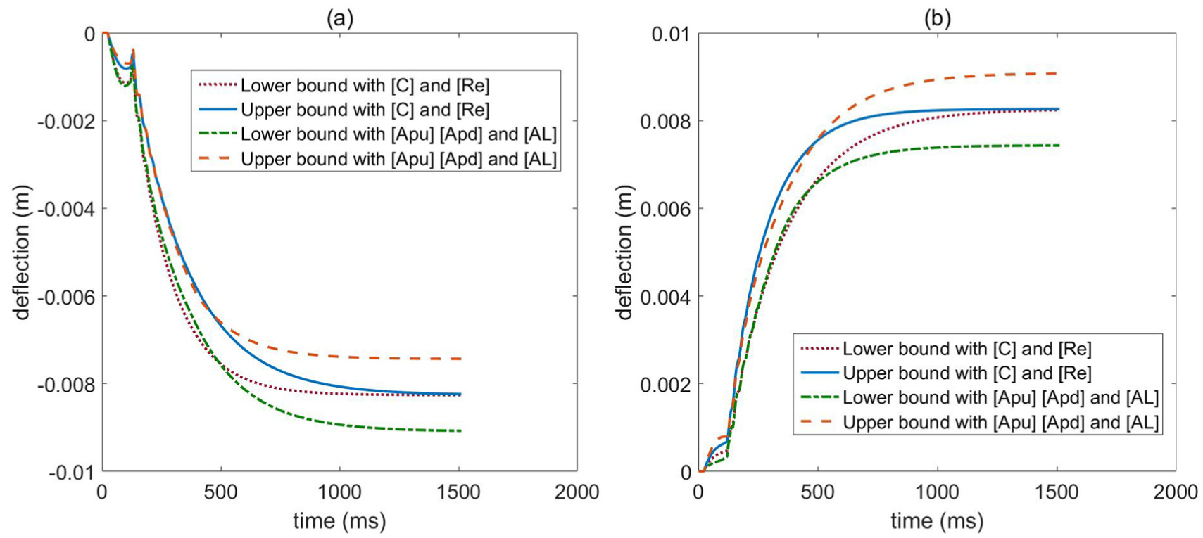
Influence comparison between the two sets of uncertain parameters in deflections: (a) the deflection on right side and (b) the deflection on left side.
In Figure 8, it can be seen that at the beginning, the influence of [C] and [Re] is larger than that of
Figure 9 shows the pressure response in the two actuators under the two sets of uncertain parameters. Different from the final stable discrepancies in the deflection responses with
Influence comparison between the two sets of uncertain parameters in pressures: (a) left upper chamber, (b) left lower chamber, (c) right upper chamber, and (b) right lower chamber.
Figure 10 illustrates the car roll responses under the two sets of uncertain parameters. The same with suspension deflection; although the pipe wall friction coefficient and the fluid damping coefficient are the interval parameters, the stable car roll of the two bounds is the same. On the contrary, the stable position of the car roll under the uncertain parameters of

Influence comparison between the two sets of uncertain parameters in car roll.
Conclusion
This article presents a new approach regarding the mathematical modeling of an active HIS with uncertain parameters by introducing the Chebyshev inclusion method. The active HIS system overcomes the drawbacks encountered by traditional passive suspension system semi-active system of lacking flexibility by adopting active hydraulic control unit and overweighs the conventional active suspension system by employing interconnection structures. What accompanies the introducing of hydraulic system in the mathematical model is the problem of uncertainty. Uncertainty would considerably degrade the veracity of a mathematical model and even make the model invalid, if not properly handled. As the pipe friction coefficient and the fluid damping coefficient are of high-level uncertainty and are hard to acquire relative accurate values, taking the advantage of the concept of interval method, a non-probabilistic method called Chebyshev interval model is proposed. Although these parameters are uncertain, the boundaries of them are relative easy to acquire.
Two sets of uncertain parameters are chosen in this article, representing the uncertainty of hydraulic systems and the uncertainty of manufacturing accuracy, respectively. To evaluate the effectiveness and accuracy of the proposed method, a thorough comparison has been conducted. Three points have been revealed and verified by the demonstration.
The presented Chebyshev interval method could solve the uncertain problem with similar accuracy but higher efficiency compared with the standard scanning method.
The possible working area which is enclosed by the upper bound and lower bound sheds light upon the necessity to conduct uncertain analysis simulation prediction with a predetermined uncertain parameter may contradict the real situation.
Footnotes
Academic Editor: Weicha Sun
Declaration of conflicting interests
The author(s) declared no potential conflicts of interest with respect to the research, authorship, and/or publication of this article.
Funding
The author(s) disclosed receipt of the following financial support for the research, authorship, and/or publication of this article: This research was partially supported by the Australian Research Council (Discovery Projects) (DP150102751) and the National Natural Science Foundation of China (11472112).