Failure assessment and life calculation of welded joints based on parameter table optimization algorithm

Abstract

In order to reduce the potential safety hazards in the operation of rail vehicles, a new parameter table optimization algorithm based on the particle swarm optimization algorithm is proposed to carry on the failure assessment and fatigue life calculation of welded joints. This algorithm reduces the number of iterations by adding connection pools to connect the parameter selection database. In addition, based on this algorithm, combined with Python language and BS7910 standard, a calculation program for failure assessment and fatigue crack growth life is written. The algorithm program is validated by taking the commonly used T-type, butt, and lap joints as examples. In terms of failure assessment, the calculation results of the algorithm program are securer and more conservative, and the safety accuracy of the algorithm program is improved by 8%–12%. In terms of fatigue crack growth life, the error between the calculated value of the algorithm program and the test data is within the engineering allowable range. At the same time, the algorithm program can give the evaluation calculation results more intuitively and quickly, which provides a reference for the failure assessment and life calculation of the welded structure.

Introduction

In the operation of railway vehicles, the fatigue fracture problem of structures is essentially a complex mechanical problem. ¹ The current research methods are mostly based on fracture mechanics theory and the derived standards such as BS7910 and ASME. Taking the BS7910 standard ² as an example, the standard includes evaluating whether the defective component is safe under the current condition according to the failure assessment diagram (FAD diagram), and giving the fatigue crack propagation residual life curve of the structure through the Paris formula and the basic theory of fracture mechanics. Nowadays, the BS7910 standard has been widely used in the fatigue resistance design of welded components.

Liu et al. ³ conducted a research on the safety evaluation method of the welding defects of the aluminum alloy car body based on the FAD diagram, and discussed whether the welding seam defects of the car body can meet the safety requirements of train operation under various a/c dimensions. Ziane et al. ⁴ put forward a mixed model for predicting the fatigue life based on the neural network optimization algorithm, and the accuracy of the model for predicting the fatigue lives of wind turbine blades was verified by comparing with the test data. Hong et al. ⁵ combined the multi-objective genetic algorithm and nominal stress method to optimize the quality of tank car frame, greatly improving its fatigue life. Li et al. ⁶ used the multi-objective optimization based on the particle swarm algorithm to improve the fatigue life of the semi-trailer tractor by optimizing the frame beam size on the basis of meeting the strength requirements. Jia et al. ⁷ compiled the C language iterative program according to the BS7910 standard, and estimated the allowable sizes of fatigue cracks of cranes under various stress conditions. Choong-Hyun et al. ⁸ combined the BS7910 standard’s systematic evaluation process for defects with first-order and second-order reliability models (Form, SORM), the reliability of a given defect structure is evaluated on the basis of considering the uncertainty of important parameters in defect evaluation. Yang et al. ⁹ carried out the secondary development of ABAQUS software combined with Python programming language, which can analyze the damage tolerance of structural parts under the action of cyclic load, and predict the fatigue lives of structural parts according to the Paris formula. Ding et al. ¹⁰ took the structure of a converter device as the research object, and used the fatigue life visualization program based on the secondary development of Ansys to conduct a global analysis and research on the fatigue life of components. Liu and Tang ¹¹ used the topology optimization algorithm to carry out the secondary development. They added or deleted the element based on the mechanical properties of the material, and decomposed the fatigue life of the three-dimensional cantilever beam to improve the optimization calculation efficiency. Hou and Wang ¹² took the long-span bridge as the research object, combined with MATLAB program to carry out the secondary development of Ansys, and realized the visualization of fatigue life and failure probability of the bridge under variable amplitude load. Lui and Chen ¹³ developed a fatigue life assessment system based on VB language, Paris formula, and Miner cumulative damage theory, which can improve the design efficiency of the crane and optimize the quality of the crane.

However, in the above analysis process, through experiments and manual calculation, the cost is high, the process is complex, and a lot of manpower and material resources are consumed, and the calculation results are inaccurate. Or the secondary development simplified calculation is only conducted for a certain type of problems, which has certain limitations. Therefore, based on the parameter table optimization algorithm and the BS7910 standard evaluation principle, this paper writes a visual program through the Python language to output the FAD diagram and the residual life curve of crack growth, effectively simplifies the process of welding joints failure assessment and the remaining life calculation. At the same time, taking T-type, butt joints, and lap joints as examples, it proves the feasibility and accuracy of the program based on the parameter table optimization algorithm, which has important practical value for the failure assessment and the prediction of fatigue life of the welded structure.

Principles of optimization algorithms

Typical parameter optimization algorithms

Typical parameter optimization algorithms are mainly divided into three categories: convex optimization parameter algorithms, intelligent optimization parameter algorithms, and black-box optimization parameter algorithms. Among them, the representatives of convex optimization arithmetic algorithms are: least squares method, Newton method, and gradient descent method. The representatives of intelligent optimization parameter algorithms are: genetic algorithm, particle swarm optimization algorithm, and ant colony algorithm. The representatives of black-box optimization parameter algorithms are: Bayesian optimization algorithm and random search optimization algorithm.

Taking the particle swarm optimization algorithm ¹⁴ in the intelligent optimization parameter algorithms as an example, it is a random search algorithm based on group cooperation summarized and proposed by Kennedy ¹⁵ and Eberhart ¹⁶ by simulating the predation behavior of birds.

In the particle swarm optimization algorithm, the solution of each optimization problem is regarded as a bird in the solution space, which called “particle.” Each particle reaches its individual optimal solution through multiple searches in the solution space, ¹⁷ the particle swarm determines the position of the global optimal solution through the individual optimal solution searched by each particle, and makes each particle adjust the connection of the next search. Finally, the optimal solution of the particle swarm optimization algorithm can be found through the above-mentioned multiple iterative search processes. ¹⁸

The principle of the particle swarm optimization algorithm is to initialize a group of random particles, record their current positions, and then determine the search direction and distance of each particle at a given speed, namely:

$${\mathrm{X}}_{\mathrm{i}}={\mathrm{X}}_{\mathrm{i}1},{\mathrm{X}}_{\mathrm{i}2},\dots {\mathrm{X}}_{\mathrm{in}}$$

(1)

$${\mathrm{V}}_{\mathrm{i}}={\mathrm{V}}_{\mathrm{i}1},{\mathrm{V}}_{\mathrm{i}2},\dots {\mathrm{V}}_{\mathrm{in}}$$

(2)

In the formula, i represents the i-th particle, X_i represents the current position vector of the i-th particle, and V_i represents the current velocity vector of the i-th particle.

Each particle will find its own corresponding individual optimal solution in each iterative search process, and then search for the global optimal solution of the previous iterative process through comparison, namely:

$$\mathrm{Pbes}{\mathrm{t}}_{\mathrm{i}}=\mathrm{Pbes}{\mathrm{t}}_{\mathrm{i}1},\mathrm{Pbes}{\mathrm{t}}_{\mathrm{i}2},\dots \mathrm{Pbes}{\mathrm{t}}_{\mathrm{in}}$$

(3)

$$\mathrm{Gbes}{\mathrm{t}}_{\mathrm{i}}=\mathrm{Gbes}{\mathrm{t}}_{\mathrm{i}1},\mathrm{Gbes}{\mathrm{t}}_{\mathrm{i}2},\dots \mathrm{Gbes}{\mathrm{t}}_{\mathrm{in}}$$

(4)

In the formula, $\mathrm{Pbes}{\mathrm{t}}_{\mathrm{i}}$ represents the individual optimal solution of the previous iterations of the particle, and $\mathrm{Gbes}{\mathrm{t}}_{\mathrm{i}}$ represents the global optimal solution corresponding to the previous iterations of the particle swarm. The particle swarm will update and optimize the particles by using the values $\mathrm{Pbes}{\mathrm{t}}_{\mathrm{i}}$ and $\mathrm{Gbes}{\mathrm{t}}_{\mathrm{i}}$ , as well as the current position X_i and speed V_i of each particle. The iterative search update equation of the entire particle swarm is as follows ¹⁹ :

$$\begin{array}{c}\multicolumn{1}{c}{{\mathrm{V}}_{\mathrm{i}}(\mathrm{n}+1)=\omega •{\mathrm{V}}_{\mathrm{i}}\left(\mathrm{n}\right)+{\mathrm{c}}_1•\mathrm{ran}{\mathrm{d}}_1•(\mathrm{Pbes}{\mathrm{t}}_{\mathrm{i}}\left(\mathrm{n}\right)-{\mathrm{X}}_{\mathrm{i}}\left(\mathrm{n}\right))}\\ +{\mathrm{c}}_2•{\mathrm{r}}_2•(\mathrm{Gbes}{\mathrm{t}}_{\mathrm{i}}\left(\mathrm{n}\right)-{\mathrm{X}}_{\mathrm{i}}(\mathrm{n}))\hfill \end{array}$$

(5)

$${\mathrm{X}}_{\mathrm{i}}(\mathrm{n}+1)={\mathrm{X}}_{\mathrm{i}}\left(\mathrm{n}\right)+{\mathrm{V}}_{\mathrm{i}}(\mathrm{n}+1)$$

(6)

In the formula, ω represents the inertia weight, and its size affects the strength of the global and local search ability. c₁ is the individual learning factor, c₂ is the group learning factor, and we usually take c₁ = c₂ = 2. $\mathrm{ran}{\mathrm{d}}_1$ and $\mathrm{ran}{\mathrm{d}}_2$ are random numbers between [0,1], which increase the randomness of the search. n and n + 1 represent the number of iterations of the particle.

Where equation (6) represents the relationship of the position and velocity between the particle of the next iterative search and the current particle. At the same time, the particles need to be limited by the maximum speed V_max during the iterative search process to avoid exceeding the limit or blindly searching.

At present, the particle swarm optimization algorithm has been widely used in many scientific and engineering fields due to its advantages of simple principle and structure as well as no need to adjust a large number of parameters.

Parameter table optimization algorithm

The parameter table optimization algorithm is derived from the particle swarm optimization algorithm in principle, they all find the optimal solution is found through group iteration. The difference between the two is that the particle swarm optimization algorithm selects the global optimal solution of the particle swarm through multiple iterations of each particle. For some evaluation processes, when there are too many parameters to be considered, the calculation amount of multiple iterations is large, the space is occupied, and the calculation process is complicated. The parameter table optimization algorithm avoids these problems by creating a connection pool and connecting the parameters to the selected database. The iterative principle is as follows:

$$\mathrm{Gbes}{\mathrm{t}}_{\mathrm{i}}=\omega •\mathrm{V}+\mathrm{c}•\mathrm{rand}•\mathrm{opt}[{\mathrm{\Omega }}_{\mathrm{ik}}•(\mathrm{Pbes}{\mathrm{t}}_{\mathrm{ik}}-{\mathrm{X}}_{\mathrm{i}})]$$

(7)

Where $\mathrm{Gbes}{\mathrm{t}}_{\mathrm{i}}$ represents the global optimal solution of the i-th test piece. The definitions and values of ω, c, and rand are the same as those in Formula (5). V is the given search speed, which needs to be initially set manually according to the geometric dimensions of the specimen. ${\mathrm{\Omega }}_{\mathrm{ik}}$ represents the database for selecting the k-th parameter in the i-th test piece. $\mathrm{Pbes}{\mathrm{t}}_{\mathrm{ik}}$ represents the individual optimal solution corresponding to the k-th parameter in the i-th test piece, which is given by the parameter selection database. X_i represents the current position vector of the i-th test piece. Opt is a function to select the optimal value, which is not an iterative calculation, but the minimum value of each parameter database and individual optimal solution calculation results. When using the parameter table optimization algorithm for evaluation calculation, if a variety of parameters are involved, it is only necessary to connect different databases through the connection pool according to the geometry of the specimens and loading conditions, so that each particle can iterate once to select the optimal solution, which reduces the computational workload and saves scientific research workers’ time.

The core of the parameter table optimization algorithm is to create a connection pool for connecting parameter databases to reduce the frequency of iterative solutions, and this process is mainly realized through code. Some code fragments are as follows, where # is followed by the comment statements in the code:

class (object):

def__init__(self, population_size, max_steps ): #Determine the number of test pieces or evaluation points

  public Get Property( String infile ){

   InputStream = InStream.getClass ()

   getResourceAsStream ( infile ) _

   Properties Props=new Properties

   try{ Props.load ( InStream )

   driver = Props.getProperty (“driver”)

   url = Props.getProperty (“ url ”)

   name = Props.getProperty (“name”)

   password= Props.getProperty (“password”)}} #Import the connection pool to connect to the parameter databases.

   public class ConnectionPool {

   private Connection CreateConn (){ } #Create a new connection in the connection pool, and check whether there is an idle connection or whether the connection has reached the upper limit. If the number of connections does not reach the upper limit, a new connection will be established.

   public synchronized Connection getConnection (){ }} #Put the connection created by the user into the connection pool.

   public class ConnectionPoolManger {

   private Connection getConnection (String poolname ){ } #Get a parameter database connection from the specified connection pool.

   public void backconn ((String poolname, Connection conn){ } #Return the connection created by the user to the specified connection pool.

   public synchronized void release (){ }} #Create all other connections

   print(‘step: %.d, best fitness: %.5f, mean fitness: %.5f’ % (step+1, self.global_best_fitness, np.mean (fitness)))# Output the value of the solution.

Realization of parameter table optimization algorithm

According to the principle of the parameter table optimization algorithm described above, in order to realize the algorithm and reflect its advantages, this paper combines the BS7910 standard and Python language to write the algorithm as a visual program.

In the program, the output of the result image is displayed in color, so that it is easy to distinguish whether the calculation result meets the evaluation requirements. In addition, the program can be run directly under the interface of ABAQUS software, which reduces the time of repeatedly modifying crack size parameters manually. According to the functional characteristics of the program, it is mainly divided into two modules, which respectively correspond to the failure assessment using FAD diagram and the prediction calculation of fatigue crack growth life in BS7910 assessment standard. The relationship between the two modules is progressive, which is the same as the evaluation calculation of BS7910 standard. That is to say, whether the failure assessment is qualified is the premise for calculating the crack growth life. If the failure assessment of the test piece is unqualified, that is, the assessment point in the FAD diagram is not within the assessment line, the test piece does not meet the requirements for continued use, and it is unnecessary to calculate its fatigue crack growth life. On the contrary, if the test piece meets the evaluation requirements of the FAD diagram, the remaining life can be calculated.

FAD graph calculation output module

The FAD diagram (Failure Assessment Diagram) is used in the failure assessment of the specimen in the BS7910 standard. It consists of the assessment coordinate system, the failure assessment curve, and the assessment points, as shown in Figure 1.

Figure 1.

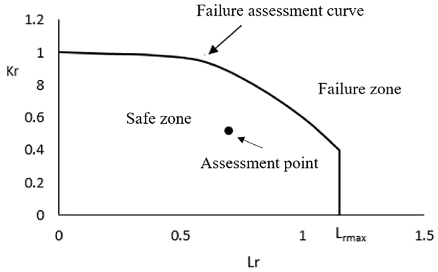
Schematic diagram of safety assessment.

In the figure, the axis of ordinate is the fracture ratio K_r, which represents the degree of failure of the structure due to brittle fracture. The axis of abscissa is the load ratio L_r, which represents the degree of instability of the structure due to plasticity. ²⁰ The limited range surrounded by the failure assessment curve and the two coordinate axes is called the safety zone. If the coordinates (L_r, K_r) of the evaluation point are located in the safety zone during the evaluation calculation, the defect is acceptable. ²¹

For the drawing of the FAD diagram, it is first necessary to select an appropriate failure assessment curve, which has three evaluation levels. Taking the commonly used 2A-level failure assessment as an example, the failure assessment line equation is:

$$\mathrm{f}\left({\mathrm{L}}_{\mathrm{r}}\right)=\{\begin{array}{c}{(1+\frac{1}{2}{\mathrm{L}}_{\mathrm{r}}^2)}^{-1/2}[0.3+0.7\exp (-{\mathrm{\mu }L}_{\mathrm{r}}^2)]{\mathrm{L}}_{\mathrm{r}}\le 1\hfill \\ \multicolumn{1}{c}{f\left(1\right){\mathrm{L}}_{\mathrm{r}}^{(\mathrm{N}-1)\left(2\mathrm{N}\right)}1<{\mathrm{L}}_{\mathrm{r}}<{\mathrm{L}}_{\mathrm{rmax}}}\\ \multicolumn{1}{c}{0{\mathrm{L}}_{\mathrm{r}}\ge {\mathrm{L}}_{\mathrm{rmax}}}\end{array}$$

(8)

In the formula, ${\mathrm{L}}_{\mathrm{rmax}}=\frac{{\sigma }_{\mathrm{s}}+{\sigma }_{\mathrm{u}}}{2{\sigma }_{\mathrm{s}}}$ , $\mathrm{\mu }=\min (0.001\frac{\mathrm{E}}{{\sigma }_{\mathrm{Y}}},0.6)$ , $\mathrm{N}=0.3(1-\frac{{\sigma }_{\mathrm{Y}}}{{\sigma }_{\mathrm{u}}})$ .

After the failure assessment curve is drawn according to the equation in the coordinate system, the coordinates of the assessment point are calculated. The first step is to calculate the fracture ratio ${\mathrm{K}}_{\mathrm{r}}$ of the assessment point. The calculation formula is:

$${\mathrm{K}}_{\mathrm{r}}=\frac{{\mathrm{K}}_{\mathrm{I}}}{{\mathrm{K}}_{\mathrm{mat}}}$$

(9)

$${\mathrm{K}}_{\mathrm{I}}=\mathrm{Y}\mathrm{\sigma }\sqrt{\mathrm{\pi }a}=[{(\mathrm{Y}\mathrm{\sigma })}_{\mathrm{p}}+{(\mathrm{Y}\mathrm{\sigma })}_{\mathrm{S}}]\sqrt{\mathrm{\pi }\mathrm{a}}$$

(10)

$$(\mathrm{Y}\mathrm{\sigma }{)}_{\mathrm{S}}={\mathrm{M}}_{\mathrm{m}}{\mathrm{Q}}_{\mathrm{m}}+{\mathrm{M}}_{\mathrm{b}}{\mathrm{Q}}_{\mathrm{b}}$$

(11)

$${\left(\mathrm{Y}\mathrm{\sigma }\right)}_{\mathrm{P}}=\mathrm{M}{\mathrm{f}}_{\mathrm{W}}\{{\mathrm{k}}_{\mathrm{tm}}{\mathrm{M}}_{\mathrm{km}}{\mathrm{M}}_{\mathrm{m}}{\mathrm{P}}_{\mathrm{m}}+{\mathrm{k}}_{\mathrm{tb}}{\mathrm{M}}_{\mathrm{kb}}{\mathrm{M}}_{\mathrm{b}}[{\mathrm{P}}_{\mathrm{b}}+({\mathrm{k}}_{\mathrm{m}}-1){\mathrm{P}}_{\mathrm{m}}]\}$$

(12)

In the formula, M represents the correction factor. f_w represents the correction factor of the finite plate width. k_m is the stress concentration factor caused by the structural dislocation. ${\mathrm{k}}_{\mathrm{tm}}$ and ${\mathrm{k}}_{\mathrm{tb}}$ are the membrane and bending stress concentration factors caused by the discontinuity of the structure. ${\mathrm{M}}_{\mathrm{km}}$ and ${\mathrm{M}}_{\mathrm{kb}}$ are the correction factors of the film and bending stress of the defect in the stress concentration zone. ${\mathrm{M}}_{\mathrm{m}}$ and ${\mathrm{M}}_{\mathrm{b}}$ are the amplification factors of film and bending stress, ²² which increase with crack size.

The second step is to calculate the load ratio ${\mathrm{L}}_{\mathrm{r}}$ of the assessment point, which is calculated as (taking the plate surface defect under normal bending constraints as an example):

$${\mathrm{L}}_{\mathrm{r}}=\frac{{\sigma }_{\mathrm{ref}}}{{\sigma }_{\mathrm{Y}}}$$

(13)

$${\sigma }_{\mathrm{ref}}=\frac{{\mathrm{P}}_{\mathrm{b}}+{[{\mathrm{P}}_{\mathrm{b}}^2+9{\mathrm{P}}_{\mathrm{m}}^2{(1-\mathrm{\alpha }″)}^2]}^{0.5}}{3{(1-\mathrm{\alpha }″)}^2}$$

(14)

$${\alpha }^{″}=\{\begin{array}{c}\frac{\mathrm{a}/\mathrm{B}}{1+(\mathrm{B}/\mathrm{c})}W\ge 2(c+B)\hfill \\ \multicolumn{1}{c}{\frac{2\mathrm{ac}}{\mathrm{BW}}W<2(c+B)}\end{array}$$

(15)

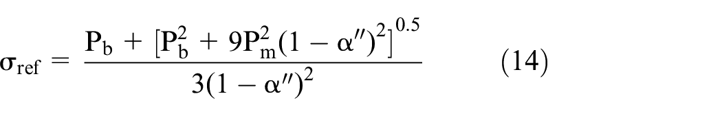
In the formula, p is the shortest distance from the surface of the component to the defect, a is the crack depth. B is the thickness of the component. W is the width of the component. ${\alpha }^{″}$ is a shape parameter related to wall thickness, pipes radius, and the crack size.

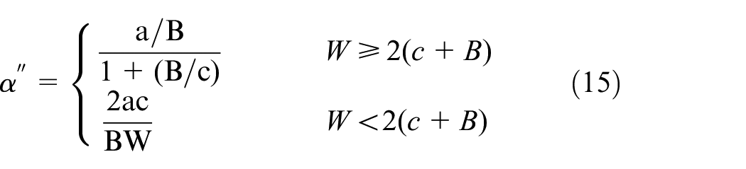
It can be seen from the above principle that in the drawing of the FAD diagram, the ordinate K_r has more influence parameters. Therefore, based on the parameter table optimization algorithm, this module writes the program by adding the parameter databases of k_m, k_tm, k_tb, and its program flow chart is shown in Figure 2. The running process of the algorithm program is as follows: After inputting the mechanical properties of the specimen material and the stress calculation results and setting the crack size, the FAD diagram can be automatically generated, and the coordinate values of the evaluation points of the FAD diagram can be output, so as to judge whether the evaluation part is damaged.

Figure 2.

Program flow chart of “FAD diagram” module.

Fatigue crack growth life calculation module

Fatigue crack growth life value is the main reference index in the fatigue assessment of the BS7910 standard. In order to accurately predict the fatigue crack growth life, it is usually necessary to obtain the fatigue crack growth rate FCGR of materials under appropriate environmental conditions through tests. However, the parameter table optimization algorithm is aimed at the optimization calculation of virtual simulation results. Therefore, in this module, the Paris formula is used to express FCGR as a function of the stress intensity factor range ΔK, so as to program the optimization algorithm. As shown in formula (16) and formula (17).

$$\frac{\mathrm{da}}{\mathrm{dN}}=\mathrm{A}(\mathrm{\Delta }\mathrm{K}{)}^{\mathrm{m}}$$

(16)

$$\mathrm{\Delta }\mathrm{K}=\mathrm{Y}(\mathrm{\Delta }\mathrm{\sigma })\sqrt{\mathrm{\pi }a}$$

(17)

Where A and m are constants, which are determined by material properties and working environment. ΔK is the range of stress intensity factor, which is a function of structural geometry, stress range and instantaneous crack size. ²³

Taking the initial crack size ${\mathrm{a}}_0$ and critical crack size ${\mathrm{a}}_{\mathrm{c}}$ as the upper and lower bounds, the integral calculation of formula (16) can be obtained:

$${\int }_0^{{\mathrm{N}}_{\mathrm{c}}}\mathrm{dN}={\int }_{{\mathrm{a}}_0}^{{\mathrm{a}}_{\mathrm{c}}}\frac{\mathrm{da}}{\mathrm{A}{(\mathrm{\Delta }\mathrm{K})}^{\mathrm{m}}}$$

(18)

In the formula; critical crack size ${\mathrm{a}}_{\mathrm{c}}=\frac{1}{\mathrm{\pi }}{\left(\frac{{\mathrm{K}}_{\mathrm{Ic}}}{\mathrm{Y}\mathrm{\sigma }}\right)}^2$ . The left side of the equation is a constant ${\mathrm{N}}_{\mathrm{c}}$ after the integral calculation, and its meaning is the life when expanding from ${\mathrm{a}}_0$ to ${\mathrm{a}}_{\mathrm{c}}$ , which is the required structural fatigue crack growth life.

In the BS7910 standard, the Paris curve is refined into two orders due to the consideration of the diversity of materials and the structural variability, and the crack propagation relationship diagram is shown in Figure 3. Figure 3(a) shows the crack propagation relationship of the first-order Paris curve, which is mostly used for conventional fatigue evaluation. Figure 3(b) shows the crack propagation relationship of the double-slope second-order Paris curve after considering the influence of welding residual stress, which is more conservative than the first-order Paris curve. ²⁴

Figure 3.

Crack propagation diagram: (a) first-order Paris curve and (b) second-order Paris curve.

Therefore, this module adds the parameter database of shape coefficient Y based on the parameter table optimization algorithm, and its program flow chart is shown in Figure 4. The running process of this program module is: After setting the mechanical properties of the materials and the relevant crack dimensions of the evaluated structure, inputting the calculated stress amplitude of the specimen and selecting the appropriate curve order, the program can output the fatigue crack growth life value and growth curve of the evaluation piece.

Figure 4.

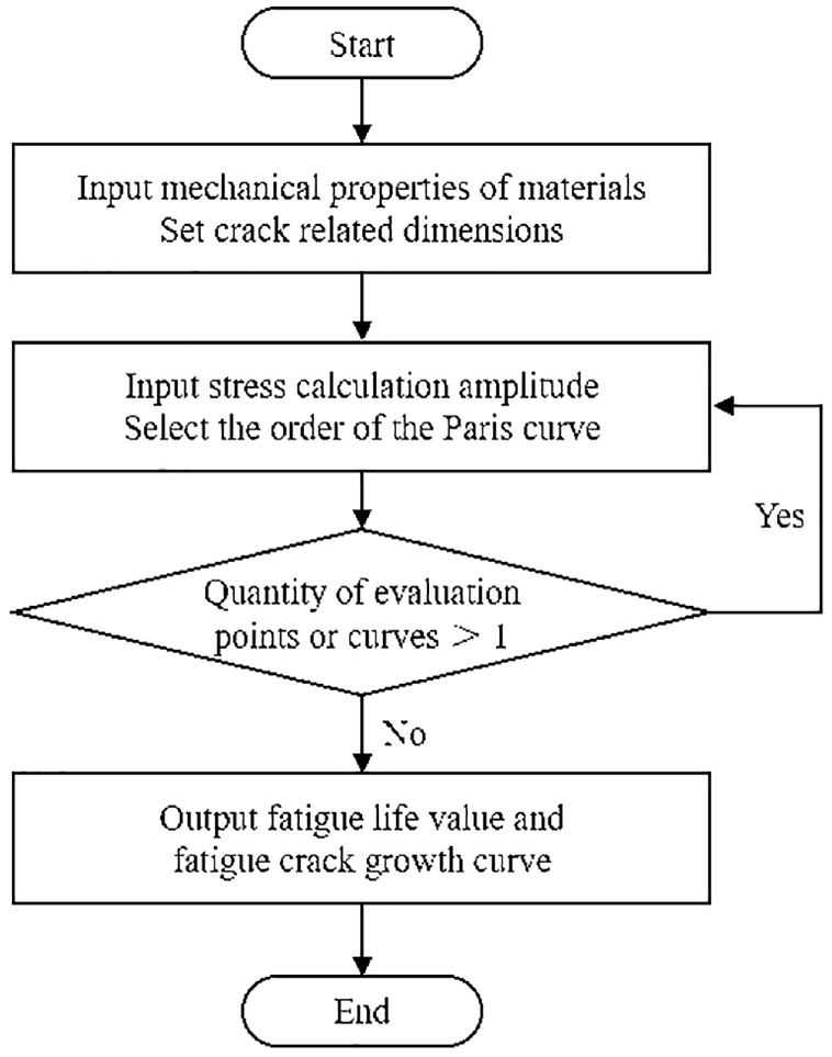
Program flow chart of fatigue crack growth life module.

Welded joint evaluation verification and result analysis

Failure assessment and verification analysis

The accuracy and practicability of the FAD diagram and fatigue crack growth life calculation program written based on the parameter table optimization algorithm needs to be verified. Taking T-type, butt, and lap joints as examples, the FAD graph calculation output module is evaluated and verified firstly.

In order to make the subsequent comparative analysis more convincing, the simulation modeling sizes of the three types of welded joints and the application data of constraints and loads are consistent with the test samples used in Refs.^25,26 Finite element models of the three types of welded joints are shown in Figure 5. For T-joints, the plate length L = 160 mm, the thickness B = 6 mm, the width W = 40 mm, the constraint is applied to the bottom plate and the two ends are 60 mm apart, and the load is applied to the center of the bottom of the weld. For butt joints, the plate length L = 160 mm, thickness B = 2 mm, width W = 30 mm, the constraint is applied on one side, the load is applied on the other side and the direction is outward stretching. For lap joints, the plate length L = 140 mm, the thickness B = 2 mm, the width W = 30 mm, the end face of the outer plate is completely fixed and the end face of the inner plate only retains the degree of freedom in the direction of force, and the tensile load is applied to the end face of the inner plate. The load application values of the three types of welded joints are shown in Table 1, and the calculation results of the stress nephogram are shown in Figure 6.

Figure 5.

Three finite element models of welded joints (unit: mm): (a) T-joint, (b) butt joint, and (c) lap joint.

Table 1.

Kr coordinate value and comparison under two calculation methods.

Specimen number	Maximum load/N	Algorithmic program calculation of Kr coordinates	Routine calculation of Kr coordinates	Accuracy improvement/%
T-1	9001	0.180	0.159	11.67
T-2	8889	0.178	0.157	11.80
T-3	7619	0.152	0.134	11.84
Butt-1	21,182	0.025	0.023	8.00
Butt-2	19,770	0.024	0.022	8.33
Butt-3	18,358	0.023	0.021	8.70
Lap-1	8499	0.049	0.044	10.20
Lap-2	7285	0.043	0.038	11.63
Lap-3	6071	0.038	0.034	10.53

Figure 6.

Stress nephogram of three types of welded joints: (a) T-joint, (b) butt joint, and (c) lap joint.

In order to reflect the superiority of the algorithm program, two methods were used to calculate the coordinate values of the evaluation points of each specimen for comparison. First, the algorithm program is used for calculation. According to the calculation results in Figure 5, in the FAD diagram calculation output module of the algorithm program, after imputing the calculated stress value in sequence and setting the relevant parameters such as material properties, the program can output the coordinate values of the evaluation points and FAD diagram, as shown in Figure 7.

Figure 7.

FAD diagram of three types of welded joints (calculated by algorithm program): (a) T-joint, (b) butt joint, and (c) lap joint.

Subsequently, the conventional failure assessment described in the Ref. ²³ is used to calculate the coordinate value of each test piece evaluation point. The coordinate value of each joint test piece evaluation point is calculated according to formula (9) and formula (13). For formula (10), the stress intensity factor of the T-joint is calculated according to formula (19) and formula (20):

$$\mathrm{F}=\frac{1.99-\alpha (1-\alpha )(2.15-3.93\alpha +2.7{\alpha }^2)}{(1+2\alpha ){(1-\alpha )}^{1.5}}$$

(19)

$${\mathrm{K}}_{\mathrm{I}}=\mathrm{F}\frac{3\mathrm{LP}}{2\mathrm{B}{\mathrm{W}}^2}\sqrt{\mathrm{\pi }\mathrm{a}}$$

(20)

where $\alpha =\mathrm{a}/\mathrm{W}$ , is the shape parameter. P is the load applied to the specimen. For butt joints and lap joints, the stress intensity factor is calculated according to Formula (21) and Formula (22):

$$\mathrm{F}(\frac{\mathrm{a}}{\mathrm{b}},\mathrm{\mu })=\frac{(1+\mathrm{\mu })}{(3+\mathrm{\mu })}\mathrm{f}\left(\frac{\mathrm{a}}{\mathrm{b}}\right)$$

(21)

$${\mathrm{K}}_{\mathrm{I}}=\mathrm{F}(\frac{\mathrm{a}}{\mathrm{b}},\mathrm{\mu })\sigma \sqrt{\mathrm{\pi }\mathrm{a}}$$

(22)

where μ is the Poisson’s ratio of the material of the joint specimen. $\mathrm{f}(\frac{\mathrm{a}}{\mathrm{b}})$ is the shape parameter, which is given by the constraint loading curve of test pieces.

Since the algorithm program only adds the parameter database of the ordinate K_r of the evaluation point in the FAD diagram calculation output module, the above two methods only compare the K_r calculation results, as shown in Table 1.

It can be seen from Figure 7, that the coordinates of the evaluation points of the three types of welded joints are all within the failure evaluation curve and no fracture occurs, so that the failure assessment is qualified. The data in Table 1 shows that the K_r value calculated by the algorithm program is larger than that obtained by routine calculation, indicating that the algorithm program after adding the parameter database is more conservative in the failure assessment. After the comparison of the two calculation methods, the accuracy of the evaluation point coordinates of each joint specimen calculated by the algorithm program is improved by 8 %–12%. Compared with the same type of development program in the Ref., ⁷ the accuracy improvement is greater.

By comparing the improved accuracy of the three types of welded joint specimens in Table 1, it is found that the calculation accuracy of the evaluation points of the butt joints has a smaller improvement than the other two types of joints. The main reasons are: the concentration degree of cyclic stress in the butt joint structure is not obvious, the weld metal bulge is small, and the stress distribution on the base metal is relatively balanced. After the surface load is applied, the maximum stress concentration point in the simulation results is displayed at the stressed end of the base metal. In the calculation of failure assessment, this position is removed as invalid data, and the stress data of the weld toe on both sides where the stress of the weld metal is relatively concentrated and the weld root are used for calculation.

According to the above conclusions, it can be seen that the results of finite element simulation and algorithm program calculation are real and effective. In terms of failure assessment, the calculation accuracy of the evaluation point coordinates calculated by the algorithm program is higher, and the output FAD diagram is more conservative and reasonable.

Verification and analysis of fatigue crack growth life

According to the assessment results given in Section 3.1 of this paper, the failure assessment of each joint specimen is qualified and meets the requirements for continued use. Therefore, we continue to calculate the fatigue crack growth life. The fatigue life of each joint specimen calculated by the algorithm program is compared with the test life to verify the fatigue crack growth life calculation module of the algorithm program. The test data of the remaining life of the three types of welded joints are provided by Refs.^25,26

Before calculating the fatigue life, it is necessary to determine the initial crack size and critical crack size of each specimen. The initial crack size a₀ of the three types of welded joint specimens is selected according to a₀/B = 0.01, that is 0.06, 0.02, and 0.02 mm. The critical crack size ${\mathrm{a}}_{\mathrm{c}}$ is calculated according to Formula (18) and needs to be compared with the plate thickness of the specimen, and the smaller of the two is taken. ²⁷ After comparison, the critical crack size of the three types of welded joints is equal to the plate thickness.

Then, according to the finite element calculation results in Figure 6, input the stress calculation amplitude and set the crack-related parameters in the algorithm program to output the fatigue life value and crack growth curve of the specimen. The fatigue crack growth curve of each joint specimen is shown in Figure 8, and the fatigue residual life test values and algorithm program calculation values are shown in Table 2.

Figure 8.

Calculation of fatigue crack growth curve by algorithmic program: (a) first-order Pairs curve of T-joint, (b) second-order Paris curve of T-joint, (c) first order Pairs curve of butt joint, (d) second-order Paris curve of butt joint, (e) first order Pairs curve of lap joint, and (f) second-order Paris curve of lap joint.

Table 2.

Experimental fatigue life value and fatigue life value calculated by algorithm program.

Specimen number	Test life/time	First-order Paris curve life/time	Second-order Paris curve life/time
T-1	988,500	613,086	451,673
T-2	2,080,000	636,576	468,273
T-3	3,760,000	1,010,966	730,046
Butt-1	66,800	51,776	40,297
Butt-2	118,700	63,682	49,154
Butt-3	166,100	79,536	60,848
Lap-1	36,741	35,424	27,992
Lap-2	62,050	56,249	43,633
Lap-3	124,525	97,195	73,764

It can be seen from Figure 8, the first-order and second-order Paris curves of each joint specimen increase monotonically and smoothly, which is consistent with the theoretical trend. At the same time, the life value of the second-order Paris curve calculated by the algorithm program is smaller than the first-order Paris life value, which is consistent with the BS7910 standard and proves that the calculation output of the algorithm program is reasonable.

At present, for the prediction of fatigue crack growth life of test pieces, the vast majority of people use Paris formula to calculate, such as the calculation methods in Refs.^9,13 However, they failed to fully consider the influence of parameters such as specimen shapes and geometric sizes when calculating, which will lead to large deviation of calculation results and affect the judgment of workers. The advantage of the parameter table optimization algorithm is that it adds the shape coefficient Y parameter selection database, which can take into account the influence of different shapes and sizes on fatigue life. At the same time, since the opt function in equation (7) selects the minimum value in the calculation results, the maximum fatigue life value can be calculated on the premise of ensuring the safe use of the test piece.

Taking the No. 2 specimen of each joint as an example, the data in Table 2 shows that the test life value is 3.26, 1.86, and 1.10 times of the first-order Paris curve calculated by the algorithm program and 4.44, 2.41, and 1.42 times of the second-order Paris curve calculated by the algorithm program. As the material of T-joint specimen is aluminum alloy, the material of butt joint and lap joint specimen is steel, according to the error multiple, it can be seen that: Under the same material, the smaller the load applied to the specimen, the smaller the life error between the test and the calculation. Under the same load condition, the life error of the steel is smaller than that of the aluminum alloy. As mentioned in Ref., ²⁷ the error of the test life and the life calculated by the algorithm program based on the simulation results is not more than 10 times, which is within a reasonable range, and the calculation result of the algorithm program is valid.

Therefore, in the fatigue crack growth life calculation module, the fatigue life calculated by the program based on the parameter table optimization algorithm is also accurate and reasonable.

Conclusions

• (1) The parameter table optimization algorithm can quickly and accurately carry on the failure assessment of the specimen through the parameter selection databases added by connection pools. At the same time, combined with the FAD diagram and fatigue crack growth curve from the program compiled by the algorithm, the state and remaining life of the specimen can be judged intuitively, and the validity of the algorithm is verified by three types of commonly used welded joints.

• (2) This algorithm is only applicable to plate parts and welded joints. For other shapes such as thin-walled, cylindrical, etc., other methods need to be selected. In addition, only three parameters are added to the parameter selection databases of this algorithm. If you want to consider the selection of other parameters, further processing is required.

• (3) The algorithm program solves the visualization problem in the evaluation process, provides a reference for the evaluation of welded structural specimens, and has important application prospects and engineering significance.