Sage Journals: Discover world-class research

Abstract

Obstacle avoidance path planning in a dynamic circumstance is one of the fundamental problems of autonomous vehicles, counting optional maneuvers: emergency braking and active steering. This paper proposes emergency obstacle avoidance planning based on deep reinforcement learning (DRL), considering safety and comfort. Firstly, the vehicle emergency braking and lane change processes are analyzed in detail. A graded hazard index is defined to indicate the degree of the potential risk of the current vehicle movement. The longitudinal distance and lateral waypoint models are established, including the comfort deceleration and stability coefficient considerations. Simultaneously, a fuzzy PID controller is installed to track to satisfy the stability and feasibility of the path. Then, this paper proposes a DRL process to determine the obstacle avoidance plan. Mainly, multi-reward functions are designed for different collisions, corresponding penalties for longitudinal rear-end collisions, and lane-changing side collisions based on the safety distance, comfort reward, and safety reward. Apply a special DRL method-DQN to release the planning program. The difference is that the long and short-term memory (LSTM) layer is utilized to solve incomplete observations and improve the efficiency and stability of the algorithm in a dynamic environment. Once the policy is practiced, the vehicle can automatically perform the best obstacle avoidance maneuver in an emergency, improving driving safety. Finally, this paper builds a simulated environment in CARLA and is trained to evaluate the effectiveness of the proposed algorithm. The collision rate, safety distance difference, and total reward index indicate that the collision avoidance path is generated safely, and the lateral acceleration and longitudinal velocity satisfy the comfort requirements. Besides, the method proposed in this paper is compared with traditional DRL, which proves the beneficial performance in safety and efficiency.

Keywords

Obstacle avoidance autonomous vehicle path planning deep reinforcement learning long and short-term memory networks

Introduction

Autonomous vehicles (AVs) can perform diverse driving tasks without a human driver, playing an essential role in improving road safety and traffic operation efficiency, and saving energy.^1,2 With the development of artificial intelligence technology, autonomous cars have become a critical research issue.³ However, a veritable traffic scenario is complicated and be still a challenging program to realize the automated system to the fully driverless period. According to statistics, about 90% of traffic accidents are caused by driver error.⁴

In a rear-end collision, the tracking vehicle brakes insufficiently due to the inability to maintain a safe distance.⁵ At the same time, the simple lane change of the ego car may conflict with other participants in the adjacent lane, which will cause a collision. The active collision avoidance system uses communication and sensor to augment the driver’s perception, transfers the acquired external information to the applicable model of the system, and takes control measures in emergencies. Thus, a practical obstacle avoidance system can help improve driving safety, including perception, decision-making, planning, and control.⁶ In addition to relying on reasonable strategies, the development of obstacle avoidance systems also requires various sensors and wireless communication technologies to realize environmental perception. This paper concentrates on the planning strategy in obstacle avoidance relying on deep reinforcement learning.

Planning a safe trajectory is a challenging problem. In fact, due to the complexity of the traffic environment, the randomness of vehicle behavior, combined with the inducing factors of rear-end collision and side collision, different maneuvering operations must be included when implementing obstacle avoidance methods, including car-following and lane-changing. In the path planning problem, traditional algorithms include A*, Artificial Potential Field (APF), and Rapidly-exploring Random Tree (RRT) is applied. The globally optimal path can be obtained in the conventional method through computing the shortest distance from the initial position to any node in the free space.⁷ As a classic breadth-first search approach, the Dijkstra algorithm searches the entire space from the initial position to the destination, resulting in heavy calculation time and data volume. The A* algorithm was proposed as a heuristic algorithm to solve the low-efficiency problem, which adds an evaluation function based on breadth-first. However, the A* algorithm fails to be applied to complex dynamic environments, and various improved methods have been designed. Liu et al. proposed the dynamic algorithm (DFPA) for pathfinding, fused Delaunay triangulation, and improved A*, processing intricate obstacles.⁸ Shang et al. designed a novel A-Star algorithm based on variable steps to reduce the calculation cost and use critical points around the obstacle to avoid the obstacle earlier.⁹

The APF path planning was a kind of virtual force method proposed by Khatib.¹⁰ It generates gravitation through the destination, obstacles generate repulsion, and finally controls the robot’s movement by seeking the resultant force. The APF is widely used due to its concise mathematical description, but it is prone to obtain the local optimum of the algorithm. In various improved researches, Hu et al. designed an improved APF method that considers vehicle speed to prevent unnecessary lane changes, and they used the gradient method to calculate the collision avoidance path of automatic driving.¹¹ Kim et al. proposed a path planning method for the APF with probability information and described the obstacles in probability.¹² Yao et al. combined reinforcement learning to solve local optimum. The potential field is used as the environment in the reinforcement learning algorithm, and the agent automatically adapts to generate a feasible trajectory.¹³

Nevertheless, the above methods all need to establish the obstacles’ model in a particular circumstance and are inappropriate for settling planning of multi-degree-of-freedom objects. The RRT method averts modeling space by performing collision checks on sampling points and effectively settles high-dimensional space and complex path planning issues. Mashayekhi et al. proposed the hybrid RRT, searching for the initial solution through bidirectional tree search and optimizing the solution.¹⁴ To be suitable for autonomous driving cars in a structured road environment, Zong et al. proposed an improved regional sampling RRT algorithm to improve search efficiency.¹⁵ Zhang et al. proposed a target bias search strategy, taking the distance and angle measurement function into account to improve the RRT algorithm and use the neural network for smoothing.¹⁶

To sum up, the classic traditional path planning method is challenging to apply to the actual traffic environment. The defined improvement method will increase the computational difficulty as the environment is complex. On the other hand, Machine Learning studies the science of using computers to simulate or realize human learning activities. A novel method of planning trajectories is through machine learning methods, but stability and optimal solutions cannot be guaranteed.¹⁷ In addition to classic algorithms and machine learning, another method is based on reinforcement learning planning.¹⁸

Reinforcement Learning (RL) is a type of machine learning that solves the agent in interacting with the environment through learning strategies to maximize returns or accomplish specific targets.¹⁹ Some researchers have applied RL to path planning, carried out related research projects, and progressed. Kim and Lee proposed real-time Q-learning without pre-stored tables and realized real-time path planning by adjusting the exploration strategy.²⁰ George integrated RRT-Q*, formulated a non-model advantage function, and used integral RL to adjust optimal strategies.²¹ Guo and Harmati proposed a semi-cooperative Nash Q-learning method based on single-agent Q-learning and Nash equilibrium, which combines game theory and RL to find the best multi-route.²² However, traditional Q-learning cannot be applied to high-dimensional states and actions; the deep Q-learning algorithm (DQN) has been developed.

Due to its versatility and the end-to-end training method, deep learning (DL) has been extensively applied in language processing, data mining, and autonomous driving. Various researches have introduced this advanced technology into path planning. Wang et al. established the DQN structure based on CNN and studied the merging of autonomous vehicle highways.² A trajectory plan combining a hierarchical reinforcement learning (HRL) structure and a PID controller was proposed to decrease the convergence time and ameliorate the generality of the algorithm.¹⁸ To solve the “dimensionality curse” problem of Q-tables, Jiang et al. established deep Q-learning based on experience replay and heuristics and demonstrated its effectiveness through simulation.²³ Koh et al. proposed a novel DRL approach to realize an effectual routing system and embedded it in the traffic simulator SUMO to realize the integration framework.²⁴ The network structure in traditional DQN is mainly based on convolutional neural networks (CNN) and recurrent neural networks (RNN). The former is mainly used for detection or classification in image processing and target detection. The latter is mainly used for processing time-series data. However, RNN is ineffective in dealing with long-term sequence problems, leading to disappearing gradients. Thus, Long Short-Term Memory (LSTM) was proposed to solve long-range dependence and used in autonomous driving research.²⁵

Vehicle collisions mainly cause traffic accidents, and any hazard avoidance scheme is defined to propose an approach to prevent crashes.²⁶ The design of active obstacle avoidance of vehicles is a challenging but meaningful issue. Therefore, this paper designs a Deep Reinforcement Learning (DRL) network using LSTM-DQN to solve obstacle avoidance path planning based on the safety distance. The integrated architecture of the method is presented in Figure 1. The ego vehicle can obtain the status of surrounding vehicles through onboard sensors (such as cameras and radars²⁷) or wireless communication. The core of our method is to use Deep Q-Network to generate a safe and comfortable obstacle avoidance path through training by introducing the safety distance of longitudinal braking and lateral lane change and Fuzzy-PID controller constraints. This paper uses the LSTM layer in the network to help the model learn from a series of observations, allowing the autonomous vehicle to learn in a more dynamic environment. Thus, the proposed approach is used to make decisions by considering multiple targets (obstacles in the current lane, surrounding vehicles in the adjacent lane). The defined special reward introduces the safety distance with different maneuvers (brake deceleration, stop waiting, lateral lane change) to ameliorate choosing beneficial obstacle avoidance operations. Finally, the DQN model is simulated and trained in open-source software. The method’s effectiveness is represented by the collision rate, total reward, trajectory curve, and vehicle parameters in different traffic scenarios.

Figure 1.

The architecture of obstacle avoidance.

The rest of this article is organized as follows. Section II introduces the background of the adopted DRL algorithm. Section III defines the obstacle avoidance behavior based on the safety distance, including the defined longitudinal braking behavior and lane-changing steering behavior, as well as Fuzzy-PID, constrained motion control. Section IV proposes the structure of DQN, including the state and action of the agent in the traffic environment, the reward based on the safety distance and the network structure of LSTM. Section V shows the agent’s performance in the simulation and the conclusion.

Deep reinforcement learning methodology

This section introduces the reinforcement learning method used in the paper, introduces the interaction between the agent and the environment.

Reinforcement learning

As a type of machine learning, RL solves the agent in interacting with the environment through learning strategies to maximize returns or accomplish specific targets.¹⁹ The common model of RL is the standard Markov Decision Process (MDP), which defines a tuple (S, A, R, p) to describe the control problem. S and A present state space and control space, respectively, R denotes the reward function, and p presents a state transition. A mapping from state sets to action sets can be expressed as: $π : S \to A$ . The action and state of the agent in the environment can be expressed as $a_{t} \in A$ and $s_{t} \in S$ at time t. The probability that the agent performs an action and transitions to the next state $s_{t + 1} \in S$ is p(s_t, a_t) with reward r_t. Since the direct addition of rewards in an infinite time series will lead to unbiased and infinite loops of states, introducing a discount factor γ makes the current reward more central than the future one.

\begin{matrix} R_{t} = r_{t + 1} + γ r_{t + 2} + γ^{2} r_{t + 3} + . . . \\ = \sum_{i = 0}^{\infty} γ^{i} r_{t + i + 1} \end{matrix}

(1)

The agent performs a in the current s, and regularly complies with strategy π to implement the operation, and obtains the state function v_π (s) and state-action function Q_π (s, a), which can be defined as:

\begin{matrix} v_{π} (s) = E_{π} [R_{t} | S_{t} = s] \\ Q_{π} (s, a) = E_{π} [R_{t} | S_{t} = s, A_{t} = a] \end{matrix}

(2)

Where π means the control policy, the optimal strategy maximizes future returns. The solution process can be roughly separated into two steps: prediction and action. The former is given a strategy to evaluate the corresponding v_π (s) and Q_π (s, a), and the latter obtains the optimal action corresponding to the current state according to the value function. Thus, the state-action function is rewritten to recursive form to update the algorithm:

Q_{π} (s, a) = E_{π} [r_{t} + γ max_{a_{t + 1}} Q_{π} (s_{t + 1}, a_{t + 1})]

(3)

The optimal policy can be derived from the state-action value function.

π (s) = \underset{a}{argmax} Q (s, a)

(4)

As an iterative process, RL has to solve two problems each time: given a policy evaluation function and update the policy according to the value function. The traditional RL finds the optimal policy by solving Bellman’s equation, that is, iteratively makes Q_π (s, a) converge to obtain the optimal strategy. However, it is expensive to use Bellman’s equation to solve the Q function in larger state space in the actual solution process.

Deep Q network

To solve iterative process costs, a neural network is used to approximate the state-action value function. First, the update function of Q-learning can be expressed as:

Q (s, a) \leftarrow Q (s, a) + α [r + γ max_{a'} Q (s', a') - Q (s, a)]

(5)

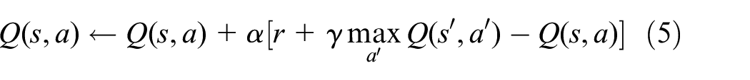
The learning rate α varying in the range [0, 1] is used to weigh the environment’s current and previous learning experience. s’ and a’ denote the state and action quantities at the immediately later procedure. The Deep Q-Network combining neural network and Q-learning was proposed to approximate the action-value function in high-dimensional state space.

Q (s, a | θ) \approx Q (s, a)

(6)

Compared with Q-Learning, except a neural network and a target Q network is introduced, DQN utilizes experience replay in training. The stochastic gradient descent (SGD) algorithm updates the network parameters in the training process and the loss function of DQN is defined as follows:

L (θ) = E [(targetQ - Q (s, a | θ))^{2}]

(7)

The optimization intent of the state-action function can be defined as:

targetQ = r + γ max_{a'} Q (s', a' | θ)

(8)

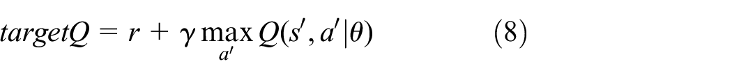
Where θ is a neural network parameter, the policy gradient method is a non-model approach optimizing the prospective total return of strategy and ferret about the optimal stratagem in the strategy space end-to-end.⁴ The greed policy chooses the action that maximizes the value function every time. Nevertheless, the states and action values that did not appear in the sampling will not be taken afterward because they are not evaluated. The ε-greedy policy combines the advantages of exploration and utilization. The rule is stochastically selected from whole actions with a probability of ε, and the best action is chosen with a probability of 1-ε.

System model

This section proposes an environment model constructed to manage the longitudinal and lateral movement of the vehicle, containing the car-following model with braking behavior and lane-changing model based on waypoints. In addition, the tracking model manages actions to perform the vehicle’s longitudinal and lateral movement behavior, respectively, based on a Fuzzy-PID controller under stable and comfortable constraints.

Environment establishment

Intelligent vehicles are an important part of the intelligent transportation system, among which planning tasks are one of the essential sections. Vehicles need to fuse multi-sensor information and realize lane-changing, lane-keeping, accelerating, or decelerating by satisfying certain constraint conditions based on driving requirements while avoiding collisions are common driving behaviors.

This paper discusses the path planning problem of autonomous vehicles; the scenario discussed is shown in Figure 1. The intelligent obstacle avoidance system should include the necessary braking and appropriate steering, and the corresponding model is established in this section. The orange car is the ego vehicle, initialized at a random speed, and prefers to move in the current lane. Defining two suspension conditions: the ego vehicle collides with surrounding participants, or the time limit is reached.

Behavior option

In the reinforcement learning of this paper, the planner specifies actions by the vehicle, including longitudinal following driving and lateral lane-changing operations, and the PID controller ensures the stability and feasibility of the trajectory. In the previous research, the IDM model of individual vehicle characteristics was a popular micro model for car-following and collision-free.²⁸ The acceleration of agents can be expressed as:

\frac{dv}{dt} = a_{max} [1 - (\frac{v {(t)}^{δ}}{v_{des}}) - {(\frac{d_{des} (v (t), Δ v (t))}{Δ d (t)})}^{2}]

(9)

Where a_max denotes the maximum acceleration, v and v_des is the speed and desired speed of the ego vehicle, t represents the current time and Δv is the relative speed, δ means an acceleration index, Δd(t) is the relative spacing at time t, and d_des is the expected distance. In this state, the expected distance is affected by the front car:

d_{des} (v (t), Δ v (t)) = d_{0} + τ v (t) + \frac{v (t) Δ v (t)}{2 \sqrt{a_{max} b_{max}}}

(10)

Where d₀ is the minimum safety spacing, τ presents the safe time interval, b_max is the maximum deceleration considering comfort. As shown in Figure 2, emergency braking is an important method that cannot avoid collisions by steering; the two vehicles brake at the same time to calculate the minimum safe spacing:

d_{0} = \frac{v^{2}}{2 a_{eb}} + (v - v_{ob}) t_{a} - \frac{{v_{ob}}^{2}}{2 a_{ob}}

(11)

Figure 2.

Longitudinal braking distance model.

The subscripts e and ob represent the ego vehicle and the front obstacle, v and a are the corresponding speed and deceleration, a_eb and a_ob are the corresponding vehicle braking deceleration, t_a is the brake acting time. The parameters of the IDM model have clear physical meanings and can visually show changes in driving behavior, describing the car-following behavior of free flow and congested flow conditions. While the relative velocity between two cars is relatively small, the slight change in the headway distance will not cause a significant deceleration.²⁹ To ensure the ego vehicle keeps following the leading vehicles under certain conditions or stops to wait for a new steering action, a graded hazard index L_h is established to plan the longitudinal movement of the vehicle.

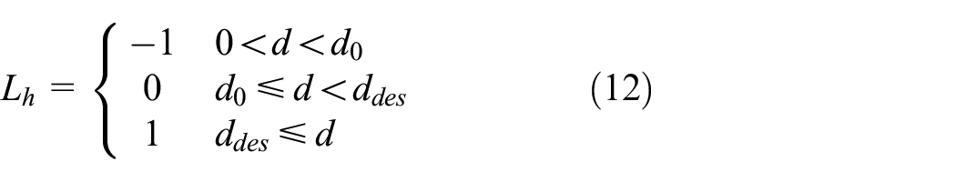
L_{h} = {\begin{matrix} - 1 & 0 < d < d_{0} \\ 0 & d_{0} \leq d < d_{des} \\ 1 & d_{des} \leq d \end{matrix}

(12)

Where d represents the actual spacing between two vehicles, L_h = −1 means danger due to the relative distance being too close, L_h = 0 means a relatively safe state, and L_h = 1 indicates the vehicle can move at the desired speed. At this time, the ego vehicle should control the speed based on the front obstacle, avoiding collisions by steering when satisfying lane-change conditions. In extreme danger, the ego vehicle decelerates to a waiting state. The tracking controller plans the candidate path according to the speed setting.

v = {\begin{matrix} 0 & L_{h} = - 1 \\ v_{ob} & L_{h} = 0 \\ v_{des} & L_{h} = 1 \end{matrix}

(13)

The lane-changing behavior of vehicles needs to meet a particular distance condition. In other words, a certain initial distance should be left before the lane change to prevent the lane-changing vehicle from colliding with objects in the adjacent lane. This paper uses waypoints to perform lane-changing operations. In addition, the stability coefficient K is divided into understeer, neutral steering, and oversteer, which is an essential factors affecting steering stability.

δ = \frac{r (1 + K u^{2})}{u / l}

(14)

Where r presents the yaw angular velocity, u presents the velocity at the center of mass, l is the wheelbase. Planning an executable path requires limiting the front wheel angle δ within a certain range. According to the relationship in Figure 3, the position of the initial waypoint x_ini can be obtained.

\frac{x}{w} = \tan δ_{max}

(15)

Figure 3.

Lateral waypoint model.

Where w is the lane width, δ_max is the maximum front-wheel angle with passenger comfortable and vehicular stability.

x_{ini} = x + 1.5 d_{0}

(16)

A new longitudinal inspection will be restarted after the ego vehicle changes lanes and drives in an adjacent lane. The terminal waypoint is determined based on the minimum safe distance. In other words, once the strategy determines the initial waypoint, a terminating waypoint x_ter will be generated at a certain distance from the target lane.

x_{ter} = x_{ini} + d_{0}

(17)

Motion control

PID controller is an optimal control algorithm that combines proportional, integral and derivative and is widely used in vehicle tracking control tasks. Fuzzy control is a computer digital control technology based on fuzzy set theory, linguistic variables, and fuzzy logic inference.³⁰ Fuzzy-PID control is based on the PID method, takes error e and error change rate e_c as input, uses fuzzy rules for reasoning and parameter adjustment to meet e and e_c for PID parameter self-tuning at different times.

\begin{matrix} e (t) = v_{des} (t) - v (t) \\ e_{c} (t) = \frac{de (t)}{dt} \end{matrix}

(18)

To realize the adaptive adjustment of PID control initial parameters k_p₀, k_i₀, k_d₀, it is necessary to determine the input variables e and e_c varying in the range [−6, 6]. In the Fuzzy-PID control, the output variables are adjustment parameters Δk_p, Δk_i, Δk_d, respectively varying in the range [−2, 2], [−0.6, 0.6], and [−0.03, 0.03]. The corresponding fuzzy rules and reasoning process are detailed in,³¹ then the controller parameters are denoted as:

\begin{matrix} k_{p} = k_{p 0} + Δ k_{p} \\ k_{i} = k_{i 0} + Δ k_{i} \\ k_{d} = k_{d 0} + Δ k_{d} \end{matrix}

(19)

Thus, in the control level, the longitudinal and lateral movements of the autonomous vehicle are constrained, and the former adjusts the speed through a proportional controller,³² which can be presented as:

v (t) = k_{p} e (t) + \frac{1}{k_{i}} \int_{0}^{t} e (t) dt + k_{d} e_{c} (t)

(20)

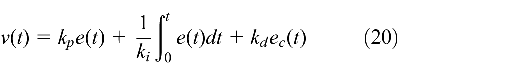
Where k_p, k_i, k_d are the gain coefficients after fuzzy method, and through accelerating or decelerating to make the speed approach the desired value.

The proportional-derivative controller realized the position and heading control in the lateral direction. The lateral speed can be presented according to the position deviation:

v_{lat} = - k_{p, lat} Δ y_{lat}

(21)

Where is k_p_,lat the position gain coefficient, Δy_lat denotes the relative lateral position based on the centerline of the lane. The relationship between the heading angle and the yaw rate is:

\overset{\cdot}{φ} = k_{d, φ} (φ_{des} - φ)

(22)

Where k_d,φ is the heading gain coefficient, φ_des is the desired heading angle. To sum up, the movement of the vehicle is realized by the control frame in Figure 1. The corresponding vehicles receive surrounding vehicles’ position, speed, and acceleration through onboard sensors or wireless communication transmissions. The following section will establish the DRL method to implement autonomous obstacle avoidance through iterative learning.

Obstacle avoidance algorithm using DRL

Action and reward

This section transforms the obstacle avoidance problem into a DRL process to determine the optimal braking and lane changing strategy in emergencies. Described in the traffic scene, lane change and emergency braking are optional actions during obstacle avoidance. The DRL-based method is suitable for learning control strategies through interaction with the environment. The ego vehicle, the front obstacle vehicle, and the surrounding environment participants are shown in Figure 1. The setting of the state space can be expressed as:

s = [v, P_{e}, v_{os}, d, L_{h}, P_{os}]

(23)

Where P_e and P_os are the position information of E and other vehicles respectively, revealing driving in the current lane or adjacent lane, v_os includes the speed of obstacle car v_ob and other participants, d is the distance of E from obstacles OB and surrounding vehicles SV, L_h is the graded hazard index introduced in the third section, describing the degree of risk of longitudinal behavior.

In the emergency obstacle avoidance problem, the vehicle speed can be planned according to the different graded indicators in the longitudinal direction. As described in the derivation, the overall strategy is to drive at the desired speed when the vehicle is safe and follow the vehicle in front within the ideal interval. Furthermore, choose the time to change lanes; otherwise, break to stop and wait for a new safe choice.

a_{o} = [a_{cf}, a_{wait}, a_{cl}]

(24)

Where a_o presents the action of an agent, the subscript cf means car-following, the subscript wait signifies the autonomous vehicle fails to meet steering conditions, performs braking and stops waiting for a new choice, and the subscript cl means lane-changing. The subsequent position and speed of the agent can be updated after time step:

\begin{matrix} x (t + Δ t) = x (t) + v_{long} Δ t + \frac{1}{2} a_{long} Δ t^{2} \\ v_{long} (t + Δ t) = v_{long} (t) + a_{long} Δ t \\ y (t + Δ t) = y_{lat} (t) + v_{lat} (t) Δ t + \frac{1}{2} a_{lat} Δ t^{2} \end{matrix}

(25)

Where x presents the longitudinal direction and y presents the lateral direction, v_long is the longitudinal speed and v_lat is the lateral speed. In RL, the agent’s target is represented as a special defined function passed to the agent through the environment, and the reward function affects the convergence accuracy and training speed. To guarantee the utility and preciseness of the obstacle avoidance system, a suitable reward function is essential.

This paper proposes the graded hazard index L_h based on the safety distance in the longitudinal direction. To facilitate the ego vehicle tending to follow safe car-following model, the longitudinal penalty function can be designed as:

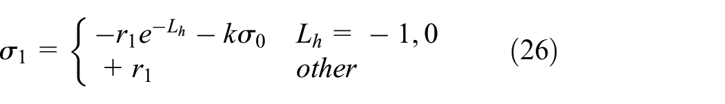
σ_{1} = {\begin{matrix} - r_{1} e^{- L_{h}} - k σ_{0} & L_{h} = - 1, 0 \\ + r_{1} & other \end{matrix}

(26)

Where r₁ is a basic penalty coefficient in this scenario, k is the collision judgment coefficient, and the value is 1 when a collision occurs; otherwise, it is 0. The obstacle avoidance system is recorded as a failure in the event of a collision, and a penalty σ₀= 100 is set at this time.

The above analysis discusses the lane change process; the current lane and adjacent lanes will be affected when the ego vehicle performs a steering operation. According to previous research, we introduce an initial safety distance formula to express the conditions for performing the steering in Figure 4.

S_{i} > L_{SV} - L_{E}

(27)

Figure 4.

Active steering condition.

Where S_i means the initial spacing, the subscript SV means the surrounding participant in the adjacent lane; the identification E indicates the autonomous agent, L indicates the longitudinal displacement and its difference between SV and E is:

S_{i} = (v_{sv} - v) t + \int_{0}^{t} \int_{0}^{t} a (τ) d τ dt + v t_{0}

(28)

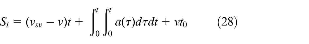
Where t₀ denotes the reaction time before braking measures, v is the longitudinal speed, t is the process current time (t≤ TTC). To prevent random lateral movement of the agent, the design of the obstacle avoidance system should first consider the longitudinal braking behavior. During the training process, If the intelligent vehicle can maintain the current lane, a certain reward will be given, defined as σ_keep.

The steering behavior is given a special reward. When the distance between the ego vehicle and vehicle in the adjacent lane is less than the safe value, the agent controls the speed according to the longitudinal behavior planned and cannot turn at this time. In the lateral direction, if the agent performs the steering failing to satisfy the limit safety spacing:

σ_{2} = - r_{2} e^{\frac{S_{i} - d}{S_{i}}} - k σ_{0}

(29)

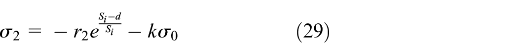
The degree of punishment is related to the actual distance and the minimum initial spacing, r₂ is a basic penalty coefficient in changing lanes, σ₂ is a collision penalty value. On the other hand, if the conditions are met, the agent can avoid collisions by changing lanes and planning lateral actions based on waypoints. In moving, passenger comfort and vehicle stability are also important parameters, and the acceleration of control behavior in the longitudinal and lateral directions is limited.

a_{long} \in [- 0.4 g, 0.4 g]

(30)

Where a_long denotes the lateral acceleration. The actual acceleration of the agent and the above restrictions a_res can form a comfort penalty function.⁴

σ_{3} = - k_{3} [(a_{e} - a_{res})^{2} + k_{4}]

(31)

Where k₃ and k₄ are weight parameters, a_e is the acceleration of the ego vehicle. In addition, this paper considers the agent and the surrounding vehicles in each episode, giving basic time step reward σ₄.

σ_{4} = + 40 / step

(32)

At the end of the episode, reaching the final position without collision is regarded as a success, and a reward will be given σ₅.

Network structure

The RNN (Recurrent Neural Network) is mainly utilized to deal with sequence data. It takes sequence data as input, recursively in the evolution direction of the sequence, and all nodes are connected in a chain-like network.³³ The advantage of RNN is that it can make full use of historical data for prediction, suitable for data scenarios where there is an apparent correlation between the front and back states.²⁵ In the design of the autonomous vehicle obstacle avoidance system, each action impacts the state at the next moment and then affects the following action. However, the traditional RNN is prone to vanishing gradients, which leads to the loss of the optimization method and the inability to optimize the model to the best results.

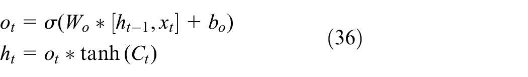
LSTM is a special kind of RNN, mainly to solve gradient disappearance and explosion during long sequence training. Compared to the standard RNN method, LSTM can perform better in longer sequences. So the state and action based on historical information can achieve more accurate predictions. Usually, x_t_-1, x_t, x_t+1 represents the input of each step, h_t_-1, h_t, h_t+1 represents the result of historical input. The first step in LSTM is to decide what information will be forgotten from the cell state.

f_{t} = σ (W_{f} * [h_{t - 1}, x_{t}] + b_{f})

(33)

Where f_t is the forget gate vector, σ is the sigmoid function, W_f and b_f represent the weight matrix. The input gate vector i_t decides to add new information to the cell.

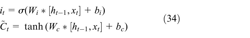
\begin{matrix} i_{t} = σ (W_{i} * [h_{t - 1}, x_{t}] + b_{i}) \\ {\tilde{C}}_{t} = \tanh (W_{c} * [h_{t - 1}, x_{t}] + b_{c}) \end{matrix}

(34)

Where W_i, W_c b_i, and b_c represent the weight matrix, C_t denotes nonlinear transformation through the hyperbolic tangent function. Then, the forget gate vector and the input gate vector work together to update the memory.

C_{t} = f_{t} * C_{t - 1} + i_{t} * {\tilde{C}}_{t}

(35)

The output gate vector can be defined as:

\begin{matrix} o_{t} = σ (W_{o} * [h_{t - 1}, x_{t}] + b_{o}) \\ h_{t} = o_{t} * \tanh (C_{t}) \end{matrix}

(36)

The Architecture of the proposed DQN algorithm based on LSTM is shown in Figure 5. The paper uses three history time steps as the input of the LSTM layer to establish the network structure (H_t= {s_t, s_t_-1, s_t_-2}). To sample the experience from the replay memory, we used the MiniBatch method to train and thus disrupt the correlation. First, the former 200 episodes of the agent are trained based on the set rules, and the results obtained are stored in the replay section. Random extraction avoids correlation problems during subsequent training in the later interaction between the environment and the agent. The action selection is based on the greedy strategy in the later interaction between the environment and the agent. After getting the action, the agent selects the waypoint with the greatest reward according to the calculation and be controlled by the defined Fuzzy-PID.

Figure 5.

DQN network structure in this paper.

Simulation and conclusion

CARLA is an open-access driving simulator that can be suitable for developing autonomous control models. In this section, simulations are processed to verify the effectiveness and preciseness of the established algorithm. The simulation uses the TensorFlow framework to run the reinforcement learning algorithm. Comprehensive efficiency and versatility, this paper selects the classic two-lane city scene that comes with CARLA as the simulation environment training algorithm based on LSTM-DQN. First, the simulation scenarios and parameter settings are shown in Table 1.

Table 1.

Corresponding parameters.

Description	Parameter	Value
Maximum acceleration	a _max	2 m/s²
Maximum deceleration	b _max	5 m/s²
Desired velocity	v _des	15 m/s
Lane width	w	4 m
Maximum front angle	δ _max	±25^o
Reaction time	t ₀	0.6 s
Brake reaction time	t_a	0.15 s
Controller parameter	k_p ₀	2
Controller parameter	k_i ₀	1
Controller parameter	k_d ₀	0.01
Penalty coefficient	r ₁	40
Collision penalty	δ ₀	100
Lane-keeping reward	σ_keep	50
Penalty coefficient	r ₂	40
Weight parameters	k ₃	0 or 1
Weight parameters	k ₄	40
Basic time step reward	σ ₄	40
Final position reward	σ ₅	1000
Discount factor	γ	0.8
Exploration rate	ε	0.001
The ego vehicle	E	Tesla Model3
The surrounding vehicle	SV	Tesla Model3
The obstacle vehicle	OB	Tesla Model3

Scenario settings

First, this paper defines an autonomous vehicle as an ego vehicle or an intelligent agent in the DRL method. The ego car needs to consider both the moving and stopping objects. We set the OB to a static state in this scene and the surrounding vehicle SV moving on the adjacent lanes. The proposed reinforcement learning algorithm plans the trajectory for car-following or lane-changing maneuvers. In other words, the ego vehicle needs to avoid collisions with obstacles as far as possible to avoid influencing the regular driving vehicles in the adjacent lanes in Figure 6.

Figure 6.

Experimental environment.

In addition, based on the consideration of randomness, the paper used the following two methods to ensure the environment of is more dynamic: the initial speed of the simulated agent is got stochastically in a range of [0 m/s, 10 m/s], and the position of the obstacle vehicle is random. The surrounding vehicles appear in adjacent lanes, and their speed is chosen from [5 m/s, 15 m/s]. The longitudinal and lateral behavior of the agent is randomly set according to the model in Section III, which can be presented as:

Emergency braking (safe distance and vehicle speed are calculated by (11) and (13) respectively. Due to the proceeding obstacle, the agent to perform car-following action or to stop to wait for the steering condition)

Active steering (the possibility of lane change exists in the adjacent lanes, the waypoint is calculated according to (16) and (17)). The agent avoids collisions by steering.

The paper uses a fixed number of history steps H_t as the input vector in the DRL simulation setting and uses the tanh activation function in the LSTM layer.¹⁸ The maximum size of the replay buffer is default 10,000. The discount rate and exploration rate of the DRL are 0.8 and 0.001, respectively. The detailed parameters are obtained in Table 1. For the weight parameter k₃ in the reward function, set it to 1 when the condition is true and 0 otherwise.⁴ We use TensorFlow to execute the experimental environment on GeForce RTX 3070.

Result analysis

The performance is illustrated by total reward and collision rate (Total reward: sum of rewards received by the agent. Collision rate: the percentage of events that have a collision in a fixed number of episodes, reflecting the algorithm’s success rate when performing obstacle avoidance). This paper defines the collision rate or degree of danger as the percentage of collisions in five episodes.

collision_rate = \sum_{i}^{i - 4} \frac{num (collision = True)}{5} (i = 5, 6, \dots)

(37)

As shown in Figure 7, due to the randomness of participants and the uncertainty of behavior in the simulated environment, the obstacle avoidance performance during the initial phase of training is poor, the ego vehicle fails to choose better driving behavior, and the possibility of collision is high (before 600 episodes, the probability of collisions is more between 40% and 80%, but the collision rate stabilizes after 450 episodes). With the iteration of training times, the collision rate gradually decreases, and the reward gradually increases (from 600 episodes to 1200 episodes, the collision probability is reduced to less than 40%). After 1200 episodes, the collision rate of the agent has been zero, and the proposed algorithm can successfully avoid a collision after training.

Figure 7.

Collision rate.

Similar to the collision rate curve, the rewards received by the agent also have a similar trend of change in Figure 8. Before 450 episodes, the reward for training is not high due to the high possibility of collision between the agent and the surrounding vehicles. Many factors affect driving safety, including the distance between the autonomous agent and the leading obstacle the position of the adjacent lane’s participants. Subsequently, as the number of training increased, the return value increased, and when it reached 1200 episodes, the value stabilized. With the iteration of training episodes, LSTM controls the transmission state through the gated state, remembering the long-term memory and forgetting the unimportant information. Finally, the algorithm achieved complete obstacle avoidance within 300 training episodes, and the reward value was high and stable.

Figure 8.

Total reward.

The blue curve in Figure 9 shows the distance between the agent and the leading obstacle of the whole training process, representing the ego vehicle’s longitudinal behavior in the obstacle avoidance operation to improve safety. In addition to the longitudinal execution of the obstacle avoidance algorithm, the brown curve describes the lane-changing behavior of the agent, except for the vehicle’s following driving or stopping and waiting for a lateral operation, which is the distance between E and SV.

Figure 9.

Distance difference.

Noting that E-OB is the spacing between agent and obstacle, and its value of 0 indicates that the agent has a rear-end collision in the longitudinal direction. Figure 9 presents that keeping the current lane without changing lanes arbitrarily is the more inclined action of the obstacle avoidance system in the starting training phase. Still, the agent fails to maintain a safe distance at this time, and frequent collisions occur. After 450 episodes, the intelligent vehicle gradually avoids collisions in the longitudinal direction and avoids collisions through active steering but maintains a specific failure rate. In episodes 450–1200, intelligent vehicles are prone to side collisions with SV when training lateral movements. After 1200 episodes, the intelligent vehicle trains longitudinal braking and lateral lane-changing operations, reducing the collision rate to 0. After that, the intelligent agent in this paper implements safe obstacle avoidance in the proposed algorithm.

There are two situations for the agent to avoid obstacles. When the adjacent lanes meet the conditions for changing lanes, the agent immediately turns actively. On the contrary, when the conditions are not met, the agent first moves to a safe distance from the obstacle and waits for the steering opportunity. Thus, in the initial training process of longitudinal behavior, the distance of E-OB fluctuates wildly. With the increase in training sets, the longitudinal distance to maintain safety tends to (11) utterly safe obstacle avoidance behavior. The E-SV distance is relatively large in the initial stage, stabilizes after 1200 episodes, and tends to (28). Finally, the obstacle avoidance behavior of the trained vehicle is realized within the set safe distance.

The trajectory and velocity reveal the control’s usefulness. (The path describes the driving route of the agent during the training process. The speed includes the longitudinal speed and the lateral acceleration, describing comfort and stability). The elaborated indicators can prove the training performance of our DRL-based method. Therefore, the experimental results and analysis of the proposed algorithm are explained in the following description.

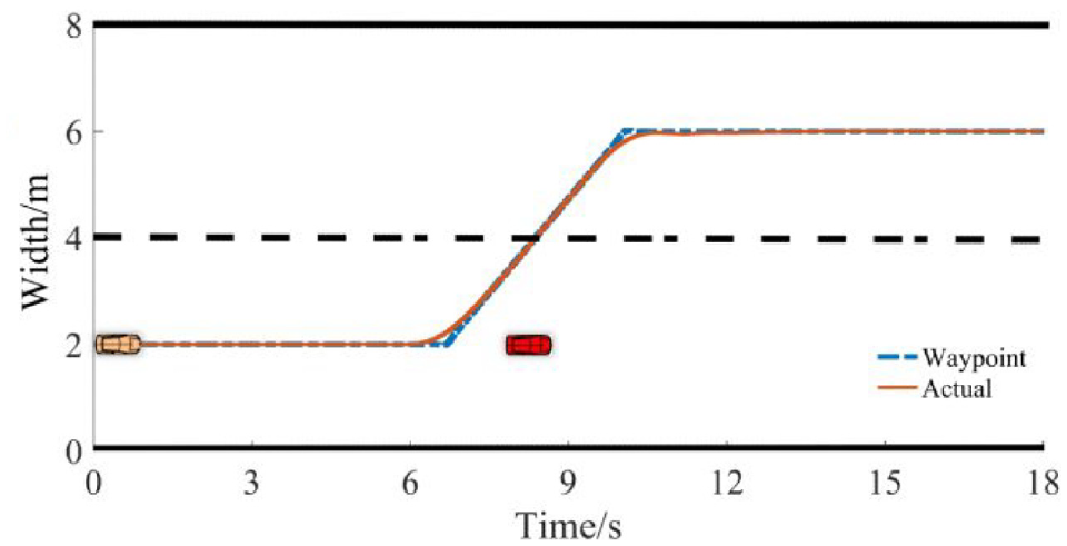
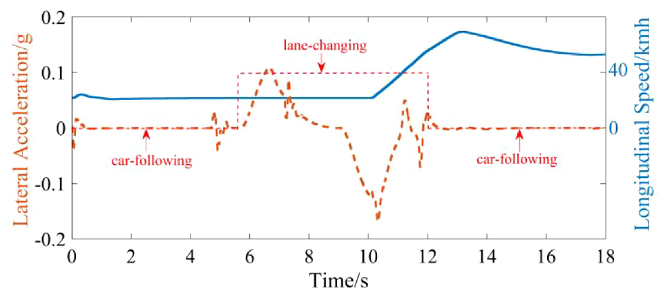
We replayed the last episode. The initial speed of the agent at the starting point is 5 m/s, there is a stationary obstacle vehicle 50 m in front, and the environmental vehicle SV is moving at a speed of 15 m/s, 40 m behind the adjacent lane. Figure 10 depicts the running conditions of two lanes with conflicts, which are the running trajectories of the agent and the surrounding vehicle. The blue dashed line is the planned waypoint. The actual brown trajectory is generated under Fuzzy-PID control, and the SV drives in a straight line in the adjacent lanes. The curve of lateral acceleration and longitudinal velocity is shown in Figure 11.

Figure 10.

The generated path.

Figure 11.

Lateral acceleration and longitudinal speed.

In the situation described, the agent first drives in the current lane at the set initial starting speed, and the algorithm checks the distance to the SV. When it moves to a position 10.1 m from the obstacle, the 14.5 m distance from the SV satisfies the lane-changing condition. The agent turns to avoid a collision at this time and accelerates to the desired speed after changing lanes. The whole process depicts an executable free lane change process, as described by the red dashed line. In the longitudinal behavior stage, the lateral acceleration fluctuates slightly. Still, it is close to 0, satisfying the constraints of maintaining the current lane driving state. The maximum lateral acceleration during the lane changing process changes within the range of 0.2g, which meets the comfort requirements.

Another classic scene in the replayed episode can be described as the ego vehicle driving at a speed of 10 m/s in the current lane. There is an obstacle 40 m ahead and a 12 m/s vehicle driving in the same position as the adjacent lane. According to (11), the agent finds that the longitudinal behavior does not meet the lane-changing condition. It first brakes and decelerates and stops at a distance of 9.09 m from the obstacle and waits for a new steering opportunity. At t = 5 s, the condition (27) is satisfied, and the agent changes lanes and accelerates to the desired speed after driving to the target lane. The complete trajectory and waypoints are shown in Figure 12.

Figure 12.

The generated path.

The obstacle avoidance process is divided into longitudinal braking and lateral lane-changing operations. The change curve of lateral acceleration and longitudinal velocity is shown in Figure 13. In the planned behavior, the maximum lateral acceleration changes within 0.2g, which will not cause passengers to be disturbed. Therefore, the obstacle avoidance planning method proposed in this paper satisfies the conditions in terms of safety and comfort.

Figure 13.

Lateral acceleration and longitudinal speed.

To further verify the performance of the proposed method, we also compare it with the traditional DRL. This paper mainly focuses on the spacing difference between participants and reward values of the two methods. The average E-OB is the distance from the obstacle when the vehicle steers, and the average E-SV is the distance from the SV when the vehicle is steering, which is used to reflect the safety performance. The average reward reflects the adaptability of the algorithm in a dynamic environment. Since we introduce the defined distance model in the reward function, the algorithm can avoid obstacles within a safe range and use LSTM to improve adaptability in a dynamic environment. The result is shown in Figure 14; compared with the traditional DQN, both the longitudinal braking behavior and the lateral lane change operation are better in terms of safety distance. Due to the LSTM network, the proposed DRL solves long-term dependence and gradient disappearance problems, improving the algorithm’s applicability and computational efficiency. So the agent obtains higher rewards in the environment.

Figure 14.

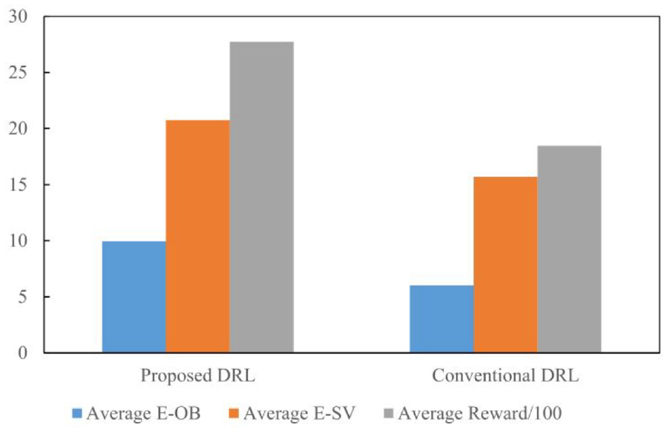
Algorithm comparison.

Conclusion

This work proposes a path planning method based on deep reinforcement learning to solve autonomous vehicles’ obstacle avoidance planning problems in emergencies. Obstacle avoidance planning is a significant research problem to reduce traffic accidents and personal injuries. This paper is based on the deep reinforcement learning-DQN method to achieve this goal. The difference is that based on comfort and safety factors, a longitudinal braking distance model and a lateral lane-changing waypoint model are established, and a hierarchical hazard index is designed to indicate driving safety, which is introduced into the reward function of DQN. After sufficient training, obstacle avoidance planning under the safe distance range is realized. In addition, the LSTM structure is used in the DQN network. The historical information of a fixed step is employed as an input to improve the model’s predictive ability and apply it to a dynamic environment. Finally, through simulation and training, the proposed obstacle avoidance plan selects appropriate actions in the longitudinal and lateral behaviors, generates a safe trajectory, and the vehicle response parameters are within the constraint range to content the comfort and stability requirements.

Footnotes

Handling Editor: Chenhui Liang

Declaration of conflicting interests

The author(s) declared no potential conflicts of interest with respect to the research, authorship, and/or publication of this article.

Funding

The author(s) received no financial support for the research, authorship, and/or publication of this article.

ORCID iD

Song Feng

References

Raj

Kumar

Bansal

A multicriteria decision making approach to study barriers to the adoption of autonomous vehicles. Transp Res Part A Policy Pract 2020; 133: 122–137.

Wang

Yuan

Guo

, et al. A deep reinforcement learning-based approach for autonomous driving in highway on-ramp merge. Proc IMechE, Part D: J Automobile Engineering 2021; 235: 2726–2739.

Rasouli

Tsotsos

JK.

Autonomous vehicles that interact with pedestrians: a survey of theory and practice. IEEE Trans Intell Transp Syst 2020; 21: 900–918.

, et al. A decision-making strategy for vehicle autonomous braking in emergency via deep reinforcement learning. IEEE Trans Veh Technol 2020; 69: 5876–5888.

Xiang

Qin

Xiang

Research on a DSRC-based rear-end collision warning model. IEEE Trans Intell Transp Syst 2014; 15: 1054–1065.

Hoel

Katherine

Wolff

, et al. Combining planning and deep reinforcement learning in tactical decision making for autonomous driving. IEEE Trans Intell Vehicles 2020; 5: 294–305.

Tsai

, et al. Combining turning point detection and Dijkstra’s algorithm to search the shortest path. Adv Mech Eng 2017; 9: 1–12.

Liu

, et al. A dynamic fusion pathfinding algorithm using Delaunay triangulation and improved A-Star for Mobile Robots. IEEE Access 2021; 9: 20602–20621.

Shang

Dai

Nie

, et al. An improved A-Star based path planning algorithm for autonomous land vehicles. Int J Adv Robot Syst 2020; 17: 591–C617.

10.

Khatib

Real-time collision avoidance for manipulators and mobile robots. Int J Rob Res 1986; 5: 90–98.

11.

Zhang

Sheng

, et al. An improved artificial potential field model considering vehicle velocity for autonomous driving. IFAC-PapersOnLine 2018; 51: 863–867.

12.

Kim

Heo

Wei

, et al. A path planning algorithm using artificial potential field based on probability map. In: 2011 8th International conference on ubiquitous robots and ambient intelligence (URAI), Incheon, Korea (South), 23–26 November 2011, pp.41–43. New York: IEEE.

13.

Yao

Zheng

, et al. Path planning method with improved artificial potential Field-A reinforcement learning perspective. IEEE Access 2020; 8: 135513–135523.

14.

Mashayekhi

Idris

MYI

Anisi

, et al. Hybrid RRT: a semi-dual-tree RRT-Based motion planner. IEEE Access 2020; 8: 18658–18668.

15.

Zong

Han

Zhang

, et al. Research on local path planning based on improved RRT algorithm. Proc IMechE, Part D: J Automobile Engineering 2021; 235: 2086–2100.

16.

Zhang

Xiong

, et al. Path planning for mobile robot based on modified rapidly exploring random tree method and neural network. Int J Adv Robot Syst Epub ahead of print 24 June 2018. DOI: 10.1177/17298814187842.

17.

Osa

Pajarinen

Neumann

, et al. An algorithmic perspective on imitation learning. Found Trends Robot 2018; 7: 1–179.

18.

Naveed

Qiao

Dolan

JM.

Trajectory planning for autonomous vehicles using hierarchical reinforcement learning. Epub ahead of print 19 September 2021. DOI: 10.1109/ITSC48978.2021.9564634.

19.

Msf

Smg

, et al. Reinforcement and deep reinforcement learning for wireless Internet of Things: a survey. Computer Communications 2021; 178: 98–113.

20.

Kim

Lee

Real-time path planning through q-learning’s exploration strategy adjustment. In: 2021 International conference on electronics, information, and communication (ICEIC), Jeju, Korea (South), 31 January–3 February 2021, pp.1–3. New York: IEEE.

21.

Kontoudis

Vamvoudakis

KG.

Kinodynamic motion planning with continuous-time Q-Learning: an online, Model-Free, and Safe Navigation Framework. IEEE Trans Neural Netw Learn Syst 2019; 30: 3803–3817.

22.

Guo

Harmati

Evaluating semi-cooperative Nash/Stackelberg Q-learning for traffic routes plan in a single intersection. Control Eng Pract 2020; 102: 104525.

23.

Jiang

Huang

Ding

Path planning for intelligent robots based on deep Q-learning with experience replay and heuristic knowledge. IEEE-CAA J Automatic 2020; 7: 1179–1189.

24.

Koh

Zhou

Fang

, et al. Real-time deep reinforcement learning based vehicle routing and navigation. Appl Soft Comput 2020; 96: 106694.

25.

Hochreiter

Schmidhuber

Long short-term memory. Neural Comput 1997; 9: 1735–1780.

26.

Khajepour

Melek

, et al. Path planning and tracking for vehicle collision avoidance based on model predictive control with multiconstraints. IEEE Trans Vehicular Technol 2017; 66: 952–964.

27.

Islam

Hossan

Jang

YM.

Convolutional neural network scheme-based optical camera communication system for intelligent internet of vehicles. Int J Distrib Sens Netw Epub ahead of print 18 April 2018. DOI: 10.1177/1550147718770.

28.

Sun

Zheng

Sun

The relationship between car following string instability and traffic oscillations in finite-sized platoons and its use in easing congestion via connected and automated vehicles with IDM based controller. Transp Res Pt B Methodol 2020; 142: 58–83.

29.

Xiong

Wang

Zhang

, et al. Combining deep reinforcement learning and safety based control for autonomous driving, https://arxiv.org/abs/1612.00147 (2016).

30.

Chen

Zhang

, et al. Adaptive speed control method for electromagnetic direct drive vehicle robot driver based on fuzzy logic. Meas Control 2019; 52: 1344–1353.

31.

Shim

Adireddy

Yuan

Autonomous vehicle collision avoidance system using path planning and model-predictive-control-based active front steering and wheel torque control. Proc IMechE, Part D: J Automobile Engineering 2012; 226: 767–778.

32.

Liao

Liu

Tang

, et al. Decision-making strategy on highway for autonomous vehicles using Deep Reinforcement Learning. IEEE Access 2020; 8: 177804–177814.

33.

Shao

Delay-dependent stability for recurrent neural networks with time-varying delays. IEEE Trans Neural Netw 2008; 19: 1647–1651.

Obstacle avoidance planning of autonomous vehicles using deep reinforcement learning

Abstract

Keywords

Introduction

Deep reinforcement learning methodology

Reinforcement learning

Deep Q network

System model

Environment establishment

Behavior option

Motion control

Obstacle avoidance algorithm using DRL

Action and reward

Network structure

Simulation and conclusion

Scenario settings

Result analysis

Conclusion

Footnotes

Declaration of conflicting interests

Funding

ORCID iD

References